Computer-assisted proofs in geometry and physics

Computer-Assisted Proofs in Geometry and Physics

by

Gregory T. Minton

Submitted to the Department of Mathematics

in partial fulfillment of the requirements for the degree of

Doctor of Philosophy

at the

MASSACHUSETTS INSTITUTE OF TECHNOLOGY

September 2013

ARCHNB~

MASSACHUsET S INSTflhrE OF TECHNOLOGY

-EP

112013

LIBRARIES

@ Gregory T. Minton, MMXIII. All rights reserved.

The author hereby grants to MIT permission to reproduce and to distribute publicly

paper and electronic copies of this thesis document in whole or in part in any medium

now known or hereafter created.

Author ...

4rtment .ofkamatics

August 16, 2013

C ertified by ...

.. ... .. L ...

Abhinav Kumar

Associate Professor of Mathematics

Thesis Supervisor

A ccep ted b y ...

Paul Seidel

Co-Chairman, Department Graduate Committee

Computer-Assisted Proofs in Geometry and Physics

by

Gregory T. Minton

Submitted to the Department of Mathematics on August 16, 2013, in partial fulfillment of the

requirements for the degree of Doctor of Philosophy

Abstract

In this dissertation we apply computer-assisted proof techniques to two problems, one in discrete geometry and one in celestial mechanics. Our main tool is an effective inverse function theorem which shows that, in favorable conditions, the existence of an approximate solution to a system of equations implies the existence of an exact solution nearby. This allows us to leverage approximate computational techniques for finding solutions into rigorous computational techniques for proving the existence of solutions.

Our first application is to tight codes in compact spaces, i.e., optimal codes whose optimality follows from linear programming bounds. In particular, we show the existence of many hitherto unknown tight regular simplices in quaternionic projective spaces and in the octonionic projective plane. We also consider regular simplices in real Grassmannians.

The second application is to gravitational choreographies, i.e., periodic trajectories of point particles under Newtonian gravity such that all of the particles follow the same curve. Many numerical examples of choreographies, but few existence proofs, were previously known. We present a method for computer-assisted proof of existence and demonstrate its effectiveness by applying it to a wide-ranging set of choreographies.

Thesis Supervisor: Abhinav Kumar Title: Associate Professor of Mathematics

Acknowledgments

First and foremost, cliched though it may be, I would like to thank my parents: they were always around, through every up and every down. I also thank my MIT advisor, Abhinav Kumar, and my Microsoft Research mentor, Henry Cohn. They encouraged and enabled me to pursue complete awesomeness at all times. Along the way I have benefited greatly from the friendship of my officemates and fellow graduate students - especially Peter, John, and Sam, who probably could have written two theses each if I had stopped distracting them

-as well -as my friends outside the department, especially Scott, Nora, J-ason, and Lisa; thank you all. I also want to acknowledge Sara, who had a big influence on this thesis.

Finally, this is for James, who would have done it all better.

I also thank the Fannie and John Hertz Foundation for, together with a National Science Foundation

Contents

I Introduction 9

1 Computer-Assisted Proof . . . . 9

2 An Effective Existence Theorem . . . . 9

2.1 Related existence theorems . . . . 13

3 Computational Considerations . . . . 13

3.1 Choice of norm . . . . 13

3.2 Interval arithmetic . . . . 14

II Optimal simplices and codes in projective spaces 17 1 Introduction . . . . 17

2 Codes in Projective Spaces . . . . 18

2.1 Projective spaces over R, C, H and ( . . . . 18

2.2 Tight simplices . . . .

.

.

. . . . . ... . . . . . . .. 20

2.3 Linear programming bounds . . . 21

2.4 Tight codes in RP-l . . . . 25

2.5 Tight codes in CP-l . . . . 26

2.6 Tight codes in H pdl and 1P2 . . . . 27

2.7 Gale duality . . . . 27

3 Simplices in Quaternionic Projective Spaces . . . . 29

3.1 Generic case . . . . 29

3.2 12- and 13-point simplices . . . . 33

3.3 15-point simplices . . . . 35

4 Simplices in Bp2 . . . . 38

4.1 Generic case . . . . 38

4.2 24- and 25-point simplices . . . . 40

4.3 27-point simplices . . . 41

5 Simplices in Grassmannians G(m, n, R) . . . . 42

5.1 Miscellaneous special cases in Grassmannians . . . . 45

6 Algorithms and Computational Methods . . . . 48

6.1 Rigorous proof . . . . 48

6.2 Finding approximate solutions . . . . 49

6.3 Finding stabilizers . . . . 50

6.4 Real algebraic numbers . . . 51

6.5 Estimating dimensions . . . 51

7 Explicit Constructions . . . . 52

7.1 Two universal optima in SO(4) . . . . 52

IIIGravitational Choreographies I Background . . . . 1.1 Periodic orbits . . . . 1.2 Choreographies . . . . 1.3 Figure-eight . . . . 1.4 Variational proofs . . . . 1.5 More choreographies . . . . 1.6 Non-variational approaches . . . . 2 Formal Problem Statement . . . .

2.1 Physics . . .. . . ' . .. .. . . . .. . . . .

2.2 Conserved quantities . . . .

2.3 Normalization . . . . 2.4 Fourier series representation . . . .

2.5 The action and its gradient . . . .

3 O ur Results . . . .

3.1 Proving existence of choreographies . . . . 3.2 Finding choreographies numerically . . . .

3.3 Saddle points of the action . . . . 3.4 Identifying real orbits . . . .

3.5 Symmetry . . . .

3.6 Stability . . . . 4 Our Proof Technique . . . . 4.1 Action principle . . . .

4.2 Expressions for the gradient and Hessian . . . . . 4.3 Computing bounds on functions and their Fourier 4.4 Step 1: bounding the gradient . . . .

4.5 Step 2: accounting for symmetries . . . . 4.6 Step 3: bounding the Hessian . . . . 4.7 Step 4: bounding the change in the Hessian . . .

4.8 Final bounds . . . .

5 Implementation Details . . . .

5.1 Optimizations in Hessian computations . . . . . 5.2 Dropping variables . . . .

5.3 Computing bounds on Fourier coefficients . . . .

5.4 Faster matrix multiplication . . . .

6 Comparison With Previous Work . . . .

6.1 Kapela et al.'s computer-assisted proofs . . . . .

6.2 Arioli et al.'s computer-assisted proofs . . . .

6.3 Treatment of symmetries . . . . 7 Further Work . . . . 8 Gravitational Gallery . . . . coefficients 61 61 62 62 63 64 67 69 71 71 72 72 73 75 75 76 77 79 80 81 84 85 86 90 92 95 95 96 97 99 100 100 101 103 104 105 105 106 107 107 .111

Chapter I

Introduction

1

Computer-Assisted Proof

The role of computational results in mathematics is well-established, but its role in rigorous proof is relatively young. The first proof of the four color theorem, given in 1976 by Appel and Haken [2], is the break-out example of a proof involving computations so extensive that they cannot be checked by a human. Since then there have been many more theorems proven using extensive and essential computer calculations; two particularly noteworthy examples are the Kepler conjecture, now Hales' theorem [6], and the existence of the Lorenz attractor [19]. Even the solution of checkers [17] can be thought of as a theorem of this sort.

These are examples of computer-assisted proofs. Our work gives two applications of computer-assisted proof techniques, one in geometry (Chapter II) and one in physics (Chapter III). Of the four examples just given, our applications have more in common with the Kepler conjecture and the Lorenz attractor, as opposed to the four color theorem and the solution of checkers. For the latter pair, the problem is essentially discrete; once made finite, it is clear that a computer could address the problem, at least in principle. By contrast, the former pair, and our work, are continuous problems. It is perhaps less intuitive that computational results can resolve such problems.

Note that we distinguish computer-verified proofs from computer-assisted proofs, with our distinction being that the former involves the formal verification of proofs, whereas the latter is concerned with proving new theorems. The focus here is on new theorems, and in particular on theorems for which we know of no plausible approach avoiding the invocation of electronic computers.

Both of our applications concern the existence of objects with certain properties. More-over, in both settings there is no particular reason to suppose that these objects have a concise, explicit representation (say, in terms of low-degree algebraic numbers). But, as we shall formalize later, there is no particular reason why they should not exist; they can be viewed as solutions to systems with at least as many variables as constraints. Based on these observations, we propose that rather than existing for a "nice" reason, which could be succinctly analyzed by hand, they simply exist because ... why not?

2

An Effective Existence Theorem

The main tool for all of our computer-assisted proofs is Theorem 2.1 below. It shows that, under suitable conditions, wherever there is an approximate solution to a system of equations

there must be a true solution nearby. This result fits into a body of related work (see §2.1). It is possible that this specific formulation and proof may not have previously appeared in the literature, but we make no assertions of originality.

The theorem is stated for general Banach spaces. We use standard notation: . denotes

the norm on a Banach space,

I-I

denotes the operator norm, Df(x) is the Frechet derivative of

f

at x, B(xo, F) is the open ball around xo with radius E, and idw denotes the identity

operator on W.

Theorem 2.1. Let V and W be real Banach spaces. Given x0 C V and E > 0, suppose that

f : B(xo, E) -* W is Prichet differentiable. Suppose also that T: W -+ V is a bounded linear operator such that

IjDf(x)

o T - idwjj < 1 -

HTH

-

If(xo)l

(2.1)

for all x E B(xo,E). Then there exists x, E B(xo,E) such that f(x.) = 0.

We will obtain this result as a straightforward generalization of the following effective inverse function theorem. For notational brevity we use B(r) and P(r) to denote the open ball and closed ball, respectively, around 0 E W and of radius r.

Proposition 2.2. Let W be a Banach space, fix r > 0, and suppose g: B(r) -+ W is differentiable and satisfies g(0) = 0. Suppose also that, for some y < 1,

IIDg(x)

- idw|I I y for all x E B(r). (2.2) Then g extends continuously to B(r), and there exists h: B(r(1 -y)) B B(r) such that g(h(y)) = y for all y G B(r(1 - -y)). Moreover, if the inequality in (2.2) is strict, then the image of h lies in B(r).

Proof. Define c: B(r) -4 W by

c(x) = g(x) - x.

The map c is differentiable and the operator norm of its derivative is everywhere bounded

by y. Thus the mean value inequality implies that, for any x1, x2 C B(r),

Ic(xi) - c(x2)I -Y

lxi

- x21. (2.3)

In particular, c is Lipschitz, so uniformly continuous. The same is true of g(x) = c(x) + x. As

the codomain W is complete, c and g extend continuously to B(r). Note that the Lipschitz bound (2.3) is obeyed on the entire closed ball.

Let y c

E(r(1 -

-y)) be arbitrary and define the function

u(x) = uY(x) = x + (y - g(x)) = y - c(x)

on B(r). Applying (2.3) and the triangle inequality,

lu(x)l

ly

+

Ic(x)I

< lyI

+

Y

-

sXI

r(1

- -Y) + 'mr

=

r,

so in fact u maps B(r) to itself. Moreover, for any x1, x2 E

E(r),

lu(xI)

- u(x2)I = Ic(xi) - c(x2)I 7 -xi - X21

By the Banach contraction mapping principle, u has a (unique) fixed point; but, by

definition of uy, a fixed point is exactly a preimage of y under g. Thus, letting h(y) be the fixed point of

u

= uy, we have the desired inverse function.

Now suppose that the inequality in (2.2) is (everywhere) strict. Then ic(x)I < y - xI for any x z 0, so the argument we gave to show u(B(r)) C B(r) actually proves u(B(r)) C B(r). The fixed point of u is in its image, whence the final claim follows. E

The proof just given is cribbed from a standard proof of the inverse function theorem. We note in passing that the function h in the proposition statement is actually unique, continuous, and differentiable on B(r).

Proof of Theorem 2.1. Let g(x) = f(xo + Tx) - f(xo), define -y =

1

-

1TI.

- If(xo) /e, and

set r

E/11Th|.

We have -y < 1, and (2.1) implies

y

> 0. The map T cannot be zero because

IIidw|

1; thus -y = 1 iff f(xo) = 0, but in this case the theorem statement is trivial. If instead y

E

(0,1), then apply Proposition 2.2 and take x, = o + T(h(-f(xo))). E

In this thesis we will apply Theorem 2.1 in two different settings.

In Chapter II we apply it to finite-dimensional normed vector spaces. In this setting

Df(x) is simply the Jacobian of

f

at x, and (given suitable smoothness conditions) a

successful application of the theorem also yields the dimension of the solution set. Moreover, a weaker assumption suffices.

Proposition 2.3. Let V and W be real Banach spaces. Given xO E V and

E

> 0, suppose that f : B(xo,E) -+ W is C'. Suppose also that T: W - V is a bounded linear operator such that, for all x E B(xo, E),

IIDf (x) o T - idwhl < 1. (2.4) If the cokernel of T is finite-dimensional, then the zero locus f--'(0) C B(xo, E) is a C1 manifold of dimension dim coker T. In particular, if V and W are finite-dimensional, then f -1(0) is a C' manifold of dimension dim V - dim W.

Proof. This is basically a corollary of the preimage theorem in differential geometry, but that

theorem is not usually stated in Banach spaces and so we shall give a few details. Note that (2.4) implies that, for all x E B(xo, e), Df (x) o T is invertible; this is because the power series

Zk>o(idw -Df (x)oT)k converges, and that series yields the inverse. Fix a finite-dimensional

subspace F of V lifting coker T = V/T(W). Let x, E f -1(0) c B(xo, e) be arbitrary and

write x, = T(y1) + z, with yi E W and z E F. Choose neighborhoods U1 of yi E W and

U2 of z, E F such that T(U1) + U2 c B(xo, E). Then the function q: U1 x U2 -4 W defined by q(y, z) = f(T(y) + z) is C' and the restriction of Dq(yi, zi) to W is Df(xi) o T, which is

invertible. Thus the implicit function theorem applies to q. This identifies a neighborhood of

LI E f-1(0) with a neighborhood of zi

E

F a RdimcokerT, which proves the first statement.

For the second statement, note that invertibility of Df(xo) o T implies that T is injective, and in the finite-dimensional case that means that dim coker T = dim V - dim W. D If

f

satisfies stronger smoothness conditions, then the manifold

f-1

(0) inherits the same

properties. In Chapter II we will actually always use CO functions, so the zero sets will be smooth manifolds.

In Chapter III, by contrast, we apply Theorem 2.1 in a case where we expect

f

to be a local isomorphism. In this case it is of interest to have an effective uniqueness result. We will not actually apply this result in the present document, but we enunciate it for the record.

Proposition 2.4. Let V and W be real Banach spaces and let B C V be an open, convex

set. Let f : B -- W be a C' function, and let T: W -+ V be a bounded linear operator. If

|IT o Df (x) - idvlL < 1 (2.5)

for all x E B, then f is injective on B.

Proof. Let x , y E B be arbitrary. Applied to the function T o f - idv, the mean value inequality asserts that

I(T o f)(x) - (T o f)(y) - (x - y)| ; <IT o Df(z) - idy

ll

- x - yj

for some z E B (in fact, for some z on the line segment between x and y). Thus

I(T o f)(y) - (T o f)(x)l > (1 - T o Df(x) - idvHl) - Ix - y > 0.

This proves that T o

f

is injective, so

f

is injective a fortiori. D

In the finite-dimensional setting, it is straightforward to apply Theorem 2.1. Our task is to compute an approximate right inverse T of Df(xo) and bound IDf(x) o T - idwII

for all x E B(xo, E). The first step is no obstacle (see the next paragraph), and the second step can be done simply and elegantly using interval arithmetic (see §3.2). The difficulty in applying the theorem lies in identifying which functions f to use; that is the main challenge we face in Chapter II. By contrast, in infinite-dimensional spaces, even the computational application of Theorem 2.1 is more delicate (see §111.4).

As we shall see, the freedom to choose any matrix T which is suitably close to an approximate right inverse is immensely useful. It lets us compute T via non-rigorous methods, which are much faster than, e.g., interval arithmetic calculations (see §11.6.1 and

§111.5.1).

Remark. While the conclusion of Theorem 2.1 strengthens as E decreases, the hypotheses do

not change monotonically. The bound we need to prove for I Df(x) o T - idw

I

becomes stronger, but the domain on which we need to prove it shrinks. Thus it can, and sometimes does, happen that we can verify the hypotheses of Theorem 2.1 only by choosing a smaller E.

Aside. We proved Theorem 2.1 using a fixed-point theorem, and indeed in the literature

existence results of this form tend to be proven this way. Fixed-point theorems are powerful and general. There is an alternative perspective, though, which we think is more intuitive and explanatory: in the context of Theorem 2.1, if x(t) is a solution of the initial-value problem

x'(t) -T(Df (x(t)) o T)-f(x(0)), x(O) = xo,

then x(1) satisfies f(x(1)) = 0. This differential equation is a time-rescaled continuous analog of Newton's method, and its application to existence theorems is known [14]. If

f

is C1 and W is finite-dimensional, then one can use the Peano existence theorem to find a solution to the differential equation. In the infinite-dimensional case, if

f

is C1 and its

derivative is locally Lipschitz, then the Picard existence theorem gives a solution. However, our proof avoids the need for these smoothness assumptions.

2.1

Related existence theorems

Theorem 2.1 is effectively an effective inverse function theorem, since it can be viewed as giving quantitative bounds on a neighborhood in which

f

has a (right) inverse. Such results date back to the Newton-Kantorovich theorem [8], which gives quantitative bounds on the convergence of Newton's method; see Ortega's short note [15] for an English-language proof and Moore and Cloud's textbook [12] for a development from the computational perspective. Kantorovich's result is close in spirit to our theorem. The main difference is that he analyzed Newton's method itself, whereas we are interested only in existence and so accept a degree of abstractness in exchange for a cleaner statement and proof.

Kantorovich's theorem shares with Theorem 2.1 the property of immediate generalization to Banach spaces. It lacks, though, the freedom we have to use an approximate right inverse T. Instead Kantorovich's theorem restricts to invertible functions and uses the actual inverse of Df. It also requires that the derivative be Lipschitz. While this is often a natural condition to check computationally (as in §111.4.7), sometimes it is more convenient to instead verify (2.1) directly (as in 11.6.1).

There are other existence theorems in the literature that are closer to ours in terms of concrete computations. One such is the Krawczyk-Moore theorem [9, 11]. (The literature tends to refer to the theorem by one of those two names, but not both. Krawczyk presented an analysis of convergence but assumed the existence of a solution, while Moore noted that existence could be deduced rather than assumed.) This theorem is very similar to ours, and in fact it is stronger than ours when restricted to the finite-dimensional setting with the supremum norm. Again, the primary difference is that we have exchanged neatness for generality. The Krawczyk-Moore theorem shares with Theorem 2.1 the flexibility to choose an approximate inverse. It also generalizes to infinite-dimensional settings, although not as easily [5]. Other results in a similar vein include the existence theorems of Miranda [10] and Borsuk [3] and Smale's analysis of Newton's method [18].

3

Computational Considerations

3.1 Choice of norm

Theorem 2.1 applies to any Banach space, so (especially in the finite-dimensional setting) we are free to choose the norm best suited to our problem. We could even choose substantially different norms on the domain and codomain, although in our work we have not exploited this particular freedom.

In Chapter II we use the f' norm and in Chapter III we use the f norm. These are both convenient choices computationally because, in addition to being easy to compute the norm of a vector (which is true of any &P norm), it is easy to compute EP -+ EP operator norms

when p = 1, oc. In particular, the f* - f* operator norm of a matrix is the maximum of the f norms of its rows, and the

e

1 -- operator norm is the maximum of the f norms of its columns. The first statement is basically obvious and the second follows from convexity (or duality).

Using the 2 norm would also be an acceptable choice, as the

e

2 +

e

2 operator norm

can be approximated efficiently. (It is the largest singular value of the matrix.) However, for any other choice of £P, even approximating the operator norm is NP-hard [7]. Indeed,

3.2

Interval arithmetic

Interval arithmetic is a standard tool in numerical analysis to control the errors inherent in floating-point computations [13]. The principle is simple: instead of rounding the results of arithmetic operations to a number that can be exactly represented in a computer, we work with intervals of representable numbers that are guaranteed to contain the correct value. This lets us offload any concerns about numerical round-off error onto the computer; it automatically tracks the errors for us.

For instance, consider a hypothetical computer capable of storing 4 decimal digits of precision. Using floating-point arithmetic, 7r would best be represented as 3.142. Using this, if we computed 2 .7r then we would get 6.284, which is obviously not correct. By contrast, interval arithmetic on the same computer would represent 7r as the interval [3.141,3.142]. Then 2 .7r would be represented by the interval [6.282, 6.284], which does contain the exact value.

In our software we use the MPF1 library to provide support for interval arithmetic [16]. That in turn relies on MPFR, a library for multiple-precision floating-point arithmetic [4]. One of the main problems with interval arithmetic is that the size of the intervals can grow exponentially with the number of arithmetic operations; this problem can be ameliorated

by increasing the precision of the underlying floating-point numbers. Thus it is a major

advantage of MPFi and MPFR that the precision can be increased arbitrarily.

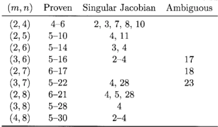
This did not turn out to be a significant issue in our applications, though. We used 128-bit floating-point numbers for the intervals in our rigorous proofs, and that proved to be sufficient in all cases save three (see Figure 111.3.1). We did not explore whether less precision would have sufficed; presumably such optimization could yield some (possibly significant) improvements in runtime.

Bibliography

[1] Noga Alon and Assaf Naor, Approximating the cut-norm via Grothendieck's inequality, SIAM J.

Comput. 35 (2006), no. 4, 787-803 (electronic). MR 2203567 (2006k:68176)

[2] Kenneth Appel and Wolfgang Haken, Every planar map is four colorable, Contemporary Mathe-matics, vol. 98, American Mathematical Society, Providence, RI, 1989, With the collaboration of J. Koch. MR 1025335 (91m:05079)

[3] Karol Borsuk, Drei sdtze iiber die n-dimensionale euklidische Sphdre, Fund. Math. 20 (1933),

no. 1, 177-190 (German).

[4] Laurent Fousse, Guillaume Hanrot, Vincent Lefevre, Patrick P lissier, and Paul Zimmermann,

MPFR: A multiple-precision binary floating-point library with correct rounding, ACM Trans.

Math. Softw. 33 (2007), no. 2.

[5] Zbigniew Galias and Piotr Zgliczyniski, Infinite-dimensional Krawczyk operator for finding

periodic orbits of discrete dynamical systems, Internat. J. Bifur. Chaos Appl. Sci. Engrg. 17

(2007), no. 12, 4261-4272. MR 2394226 (2009i:37222)

[6] Thomas C. Hales, A proof of the Kepler conjecture, Ann. of Math. (2) 162 (2005), no. 3, 1065-1185. MR 2179728 (2006g:52029)

[7] Julien M. Hendrickx and Alex Olshevsky, Matrix p-norms are NP-hard to approximate if

p

#

1, 2, oc, SIAM J. Matrix Anal. Appl. 31 (2010), no. 5, 2802-2812. MR 2740634 (2011j:15035) [8] Leonid Vitaliyevich Kantorovich, On Newton's method for functional equations, Doklady Akad.

Nauk SSSR 59 (1948), 1237-1240 (Russian).

[9] R. Krawczyk, Newton-Algorithmen zur Bestimmung von Nullstellen mit Fehlerschranken.,

Computing (Arch. Elektron. Rechnen) 4 (1969), 187-201. MR 0255046 (40 #8253)

[10] Carlo Miranda, Un'osservazione su un teorema di Brouwer, Boll. Un. Mat. Ital. (2) 3 (1940), 5-7. MR 0004775 (3,60b)

[11] Ramon E. Moore, A test for existence of solutions to nonlinear systems, SIAM J. Numer. Anal. 14 (1977), no. 4, 611-615. MR 0657002 (58 #31801)

[12] Ramon E. Moore and Michael J. Cloud, Computational functional analysis, 2nd ed., Ellis Horwood Series: Mathematics and its Applications, Woodhead Publishing, 2007.

[13] Ramon E. Moore, R. Baker Kearfott, and Michael J. Cloud, Introduction to interval analysis,

Society for Industrial and Applied Mathematics (SIAM), Philadelphia, PA, 2009. MR 2482682

(2010d:65106)

[14] J. W. Neuberger, The continuous Newton's method, inverse functions, and Nash-Moser, Amer. Math. Monthly 114 (2007), no. 5, 432-437. MR 2309983 (2008a:49037)

[15] James M. Ortega, The Newton-Kantorovich theorem, Amer. Math. Monthly 75 (1968), 658-660.

MR 0231218 (37 #6773)

[16] Nathalie Revol and Fabrice Rouillier, Motivations for an arbitrary precision interval arithmetic

and the MPFI library, Reliab. Comput. 11 (2005), no. 4, 275-290. MR 2158338 (2006e:65078)

[17] Jonathan Schaeffer, One jump ahead: computer perfection at checkers, 2nd ed., Springer, 2008. [18] Steve Smale, Newton's method estimates from data at one point, The merging of disciplines: new

directions in pure, applied, and computational mathematics (Laramie, Wyo., 1985), Springer, New York, 1986, pp. 185-196. MR 870648 (88e:65076)

[19] Warwick Tucker, A rigorous ODE solver and Smale's 14th problem, Found. Comput. Math. 2

Chapter II

Optimal simplices and codes in

projective spaces

This chapter presents joint work with Henry Cohn and Abhinav Kumar. Most of it appears verbatim in a joint paper prepared for publication [15].

1

Introduction

The study of codes in spaces such as spheres, projective spaces, and Grassmannians has been the focus of much interest recently, with an interplay of methods from many aspects of mathematics, physics, and computer science. Given a compact metric space X, the problem is how to arrange N points in X so as to maximize the minimal distance between them. A point configuration is called a code, and an optimal code C maximizes the minimal distance between its points given its size JCJ. Finding optimal codes is a central problem in coding theory. Even when X is finite (for example, the cube {O, 1}' under Hamming distance), this optimization problem is generally intractable, and it is even more difficult when X is infinite.

Most of the known optimality theorems have been proved using linear programming bounds, and we are especially interested in codes for which these bounds are sharp. We call them tight codes.1 These cases include many of the most remarkable codes known, such as the icosahedron or the E8 root system.

In this paper, we explore the landscape of tight codes in projective spaces. We are especially interested in simplices of N points in d-dimensional projective space (i.e., collections of N equidistant points). Tight simplices correspond to tight equiangular frames [39], which have applications in signal processing and sparse approximation, and they also capture interesting invariants of their ambient spaces.

In real and complex projective spaces, tight simplices occur only sporadically. All known constructions are based on geometric, group-theoretic, or combinatorial properties that depend delicately on the size N and dimension d. By contrast, we find a surprising new phenomenon in quaternionic and octonionic spaces: in each dimension, there are substantial intervals of sizes for which tight simplices always seem to exist.

'The word "tight" is used for a related but more restrictive concept in the theory of designs. We use the same word here for lack of a good substitute. This makes "tight" a noncompositional adjective, much like "optimal": codes and designs are both just sets of points, so every code is a design and vice versa, but a tight

This behavior cannot plausibly be explained using the sorts of constructions that work in real or complex spaces. Instead, the new tight simplices seem not to exist for any special reason, but rather simply because of parameter counting. Specifically, they can be characterized using more variables than constraints, in a way that suggests they should exist but does not prove it. We do not know how to prove that they exist in general, but we prove existence in many hitherto unknown cases. We also extend our methods to handle some exceptional cases that are more subtle.

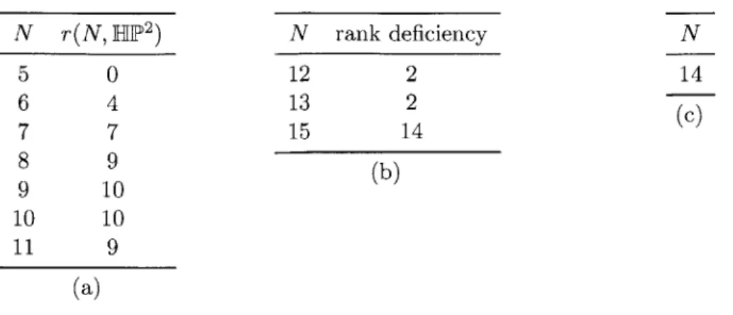
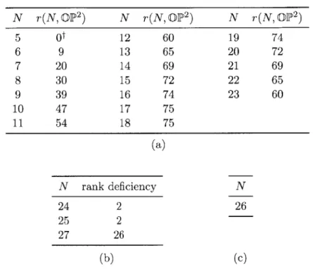
Our results settle several open problems dating back to the early 1980s. We show the existence of a 15-point simplex in HP2 and a 27-point simplex in (IP 2, which are not only

optimal codes, but also the largest possible simplices in these spaces. (For comparison, the six diagonals of an icosahedron form a maximal simplex in RP2_{, and the largest simplex in}

CP2 has size nine.) Furthermore, these simplices are tight 2-designs. We also construct a set of 13 mutually unbiased bases in (DP2_{. The mutually unbiased bases had been conjectured} to exist [24, p. 35], but no construction was known, and the tight simplices were conjectured not to exist [23, p. 251]. It would be interesting to determine whether these simplices could lead to minimal triangulations of HP2 and IP2, which would have the same number of vertices (see [10]).

We also rigorously show the existence of many tight simplices in real Grassmannians, which were conjectured to exist in [17] based on numerical evidence. This case is similar to quaternionic and octonionic projective spaces, in that parameter counts

In contrast to the usual algebraic methods for constructing tight codes, we take a rather different approach to show the existence of families of simplices. We use our general effective implicit function theorem (Theorem 1.2.1), which allows us to show the existence of a real solution to a system of polynomial equations near an approximate solution. Furthermore, when this theorem applies, it also shows that the space of solutions is a smooth manifold near the approximate solution and tells us its dimension (see Proposition 1.2.3). This allows us to establish many new results for which algebraic constructions seem out of reach.

In §2 we describe linear programming bounds and recall what is known about tight codes in projective spaces over R, C, H, and 0. Our results concerning existence of new families of simplices, proved using our main existence theorem (Theorem 1.2.1), are described in §3 and §4. In §5 we use our methods to produce several positive-dimensional families of simplices in real Grassmannians. We then give a discussion of the algorithms and computer programs used for these computer-assisted proofs in §6. Finally, we conclude in §7 with a few explicit constructions of universally optimal codes, the most notable of which is a maximal system of mutually unbiased bases in (DP2_.

2

Codes in Projective Spaces

2.1 Projective spaces over R, C, H and G

If K = _{R, C, or H, we let KPd-1 := (Kd \ {0})/KX be the set of lines in Kd. That is, we}

identify x and xa for x E Kd \ {0} and a E KX. Note the convention that KX acts on the

right; this is important for the noncommutative algebra H.

d t

We equip Kd with the Hermitian inner product (X, x2) = xix2, where

t

denotes the

conjugate transpose. We may represent an element of the projective space by a unit-length vector x E Kd, and we often abuse notation by treating the element itself as such a vector.

Under this identification, the chordal distance between two points of KPd-1 is

p(XI, x2) = 1 - (XI, x2)12.

It is not difficult to check that this formula defines a metric, which is equivalent to the Fubini-Study metric. Specifically, if t(Xi, X2) is the geodesic distance on KPd-1 under the Fubini-Study metric, normalized so that the greatest distance between two points is 7r, then

cos?9(X1, X2) = 21(xi, X2) 2 1 and

p(XI, x2) = sin (d(X1X2)).

Alternatively, elements x E KPd-l correspond to projection matrices H = xxt , which

are Hermitian matrices with H2 = 1 and Tr H = 1. The space W (Kd) of Hermitian matrices

is a real vector space endowed with a positive-definite inner product 1

(A, B) = Tr (AB + BA) = Re Tr AB.₂

Because Re ab = Re ba for a, b e K, it follows that Re Tr(ABC) = Re Tr(CAB) for A, B, C E

Kdxd; in other words, the operator ReTr is cyclic invariant. Hence, for any X1, x2 E KPd-1

with associated projection matrices

H

₁ , H₂ E '(Kd), we have

/\II, IT2) /J71~~ = Re Tr rr- mt.-lx t 2 '

= Re Trx itxizx ₂

2 1 _(2.1)

= Re (X₂, X1)(X1, x₂)

= I(Xi, X2)12

Thus the metric on KPd-1 can also be defined by p(X1, X2) = 1 - (H1 , H2). Equivalently,

it equals

H11

- 1211/v, where 11 - denotes the Frobenius norm:

|HAJH

=

(&

jAi 12)1/2

for a matrix whose i,

j

entry is Aij.

The one remaining projective space is the octonionic projective plane OP2. (See [5] for an account of why cDPd cannot exist for d > 2; one can construct CP', but we will ignore it as it is simply S8.) Due to the failure of associativity, the construction of OP2 is more complicated than that of the other projective spaces; we cannot simply view it as the space of lines in 03. However, there is a construction analogous to that in the previous paragraph. The result is an exceptionally beautiful space that has been called the panda of geometry

[8, p. 155]. The points of OP2 are 3 x 3 projection matrices over 0, i.e., 3 x 3 Hermitian matrices H satisfying H2 = H and Tr H = 1. The (chordal) metric in OP2 is given by

1

p(1, 1 2) = |IHi - H211 = 1 - (H1 , 2).

Each projection matrix H is of the form

a U1= b

(a

>B

where a, b, c E G satisfy

1a1

2 + 1bl2 + ICl2 = 1 and (ab)c = a(bc). We can cover C1P2 by

three affine charts as follows. Any point may be represented by a triple (a, b, c) E 03 with

Ja12 + 1bl2 + IC12 = 1, and for the three charts we assume a, b, or c are in R+, respectively.

In practice, for computations with generic configurations we can simply work in the first chart and refer to a projection matrix by its associated point (a, b, c) E R+ X D2.

2.2 Tight simplices

Projective spaces can be embedded into Euclidean space by identifying a point with its associated projection matrix; using this embedding, the standard bounds on the size and distance of regular simplices in Euclidean space imply bounds on simplices in projective space. The resulting bounds for regular simplices in real projective space were first proven

by Lemmens and Seidel [30]. They are also known in information theory as Welch bounds

[41].

As above, let K be R, C, H, or 0. We consider regular simplices in KPd-l, with the understanding that d = 2 when K = 0.

Definition 2.1. A regular simplex in a metric space (X, p) is a collection of distinct points

x1, ... , xN of X with the distances p(xi, xj) all equal for i

#

j.

We often drop the adjective "regular," as by a simplex we always mean a set of equidistant points.

Proposition 2.2. Consider a regular simplex consisting of N points x ₁,... , xN with asso-ciated projection matrices I1,... ,N, and let a = (ri, fj) be the common inner product for i 7 j. Then

(d2 - d) dimR K

Nd 2

and, for any such value of N,

N - d -d(N - 1)'

Proof. The Gram matrix G associated to H1, ... , HN has unit diagonal and a in each off-diagonal entry. Since G is (1 - a)IN plus a rank one matrix, an easy computation

shows det G = (1 - a)N-I(1 + (N - 1)a), which is nonzero because a E [0, 1). Thus G

is nonsingular, and the elements H1, .. ., FN E 1(Kd) are linearly independent, implying N < dimR 71(Kd) = d ± (d2 - d)(dimR K)/2. Now note that (fl1, Id) = Ixl 2 ₌

1 for each

i = 1, ... , N. Using this we compute

K

Ui d

_d

_{= N -}

_{+ N(N - 1)a.}

Nonnegativity of this expression gives the desired bound on a. El Definition 2.3. We refer to a regular simplex with

N-d d(N - 1)

as a tight simplex. That is, it is a simplex with the maximum possible distance allowed by Proposition 2.2.

Note that this definition is independent of the coordinate algebra K. In other words,

the embeddings RIpd-1 c Cpd-1 c HPd-l preserve tight simplices. Proposition 2.4. Every tight simplex is an optimal code.

More generally, the bound on a in Proposition 2.2 applies to the minimal distance of

any code, not just a simplex.

Proof. Let H1, .. ., HN be the projection matrices corresponding to any N-point code in

KPd-1. As in the proof of Proposition 2.2,

N 2 N N N N N

N

-Nd±

1

(i,Hrj)

Ili

d

Id,

(

Hi

-

dl%

Id)

>

0.

i,j=1 = =

is4i

Thus, the average of (Ii, H3) over all i z

j

satisfies

1 N N2 d - N N-d

N(N - 1) .: .Ii 'j - N(N - 1) _.d(N - 1)'

In particular, the greatest value of (Hi, H) for i #

j

must be at least this large. E A regular simplex of N < d points in KPd- is optimal if and only if the points are orthogonal (i.e., a = 0). Such simplices always exist. We only consider them to be tight

when N = d, as the N < d cases are degenerate. There also always exists a tight simplex

with N = d + 1 points, obtained by projecting the regular simplex on the sphere Sd-i into RPd-1. Therefore in what follows we will generally assume N > d + 2.

It follows immediately from the proof of Proposition 2.2 that a simplex {x1,. . ., XN is

tight if and only if

N

ZXiX~ =t jj i=1

This condition can be reformulated in the language of projective designs [20, 34] (see also [23] for a detailed account of the relevant computations in projective space). Specifically,

it says that the configuration is a 1-design. We will make no serious use of the theory of designs in this paper, and for our purposes we could simply regard Ei xx = NId as the definition of a 1-design, but we will briefly recall the general concept in our discussion of

linear programming bounds.

2.3 Linear programming bounds

Linear programming bounds [26, 20] use harmonic analysis on a space X to prove bounds on

codes in X. These bounds and their extensions [4] are one of the only known ways to prove systematic bounds on codes, and they are sharp in a number of important cases. Later in

this section we will summarize the sharp cases that are known in projective spaces (see also

Table 1 in [14] for a corresponding list for spheres), but first we will give a brief review of

how linear programming bounds work.

The simplest setting for linear programming bounds is a compact two-point homogeneous

discrete two-point homogeneous spaces such as the Hamming cube are also important in coding theory.

Let X be a sphere or projective space, and let G be its isometry group under the geodesic metric 9 (normalized so that the greatest distance is 7r). Then L2(X) is a unitary

representation of G, and we can decompose it as a completed direct sum

L2(X)= Vk k>O

of irreducible representations Vk. There is a corresponding sequence of zonal spherical

functions Co, C1,..., one attached to each representation Vk. The zonal spherical functions

are most easily obtained as reproducing kernels; for a brief review of the theory, see Sections 2.2 and 8 of [14]. We can represent them as orthogonal polynomials with respect to a measure on [-1, 1], which depends on the space X, and we index them so that Ck has degree k.

For our purposes, the most important property of zonal spherical functions is that they are positive definite kernels: for all N E N and X1,... , XN E X, the N x N matrix

(Ci(cos V(Xi, Xj))) 1<i,j<N is positive semidefinite. In fact, the zonal spherical functions span the cone of all such functions.

For projective spaces KPd-1, the polynomials Ck may be taken to be the Jacobi poly-nomials P ' , where a = (d - 1)(dimR K)/2 - 1 (i.e, a = (dimR KPd-1)/2 - 1) and

3 (dimR K)/2 - 1. We will normalize Co to be 1.

Linear programming bounds for codes amount to the following proposition:

Proposition 2.5. Let 0 E [0, r], and suppose the polynomial n

f(z) = EZfkCk(z)

k=0

satisfies fo > 0, fk > 0 for 1 < k < n, and f(z) < 0 for -1 < z < cos0. Then every code in

X with minimal geodesic distance at least 0 has size at most f(1)/fo. Proof. Let C be such a code. Then

Sf(cos 9(x,y))

foICl

2,

x,yeC

because each zonal spherical function Ck is positive definite and hence satisfies

>1

Ck (cost (x,y)) > 0. x,yeC

On the other hand, f(cos V(x, y)) 0 whenever O(x, y) > 0, and hence

)73 f(cos 7(x, y))

IClf

(1)

x,yeC

because only the diagonal terms contribute positively. It follows that foIC12 < f(1) C1, as

We say this bound is sharp if there is a code C with minimal distance at least 0 and

ICI = f(1)/fo. Note that we require exact equality, rather than just ICl = Lf(1)/foJ.

Definition 2.6. A tight code is one for which linear programming bounds are sharp.

Examining the proof of Proposition 2.5 yields the following characterization of tight codes:

Lemma 2.7. A code C with minimal geodesic distance 0 is tight iff there is a polynomial

f(z) = oE fk Ck(z) satisfying fo > 0,

fk

> 0 for 1 < k < n, f(z) < 0 for -I < z < cos 0, E Ck(cosd (x, y)) = 0

x,yc

whenever fk > 0 and k

#

0, and f(cos V(x, y)) = 0 for x, y E C with x 0 y. In fact, these

conditions must hold for every polynomial f satisfying both f(1)/fo =|C| and the hypotheses of Proposition 2.5.

By Proposition 2.5, every tight code is as large as possible given its minimal distance,

but it is less obvious that such a code maximizes minimal distance given its size.

Proposition 2.8. Every tight code is optimal.

Proof. Suppose f satisfies the hypotheses of Proposition 2.5, and C is a code of size f(1)/fo

with minimal geodesic distance at least 0. We wish to show that its minimal distance is exactly 0.

By Lemma 2.7

(f (costd(x, y)) - fo)

= 0

xyEC

and f (cosO(x, y)) = 0 for x, y E C with x

$

y

Now suppose C had minimal geodesic distance strictly greater than 0, and consider a small perturbation C' of C. It must satisfy

E (f(cos 9(x,y)) - fo) > 0, x,yec'

by positive definiteness. On the other hand,

(f(cosd(x, y)) - fo) = 1C'lf(1) - IC'l2fo + f (cos 9(x, y)).

x,yeC' x,yCc'

x~y

We have

IC'If

(1) -

IC'l

2_{fo = 0 since}

_IC'J

_{= ICI =}

f(1)/fo.

Thus, E f(cosd (x, y)) > 0.

x,yEC'

If the perturbation is small enough, then f(cos 0(x, y)) < 0 for distinct x, y E C'. In that

case, we must have f(cos

O(x,

y)) = 0 for distinct x, y e C'. However, this fails for some

perturbations, for example if we move two points slightly closer together. It follows that every code of size f(1)/fo and minimal geodesic distance at least 0 has minimal distance exactly 0, so these codes are all optimal. E

Lemma 2.9. Tight simplices in projective space are tight codes.

Proof. Up to scaling, the first-degree zonal spherical function C1 on KPd-1 is z + -d2 . Now

let

f(Z) - 1+ (N-1)d _d-2

2(d - 1) d

It satisfies f(z) < 0 for z E [-1, 2a - 1], where N-d d(N - 1)'

and f(1)/fo = N, as desired. E

Note that in this proof C1 depends only on d, and not on K. zonal spherical functions for KPd-1 depend on both d and K.

A t-design in X is a code C C X such that for every

f

E Vk

By contrast, higher-degree

with 0 < k < t,

f(x)

=

0.

XEC

In other words, every element of Vo e ... D V has the same average over C as over the

entire space X. (Note that all functions in Vk for k > 0 have average zero, since they are orthogonal to the constant functions in V.) Using the reproducing kernel property, this can be shown to be equivalent to

3

Ck (cos' (x, y)) = 0 xYEC

for 0 < k < t.

In KPd-I, one can check that

N

N XiX=-Id

1 d

holds if and only if {xi, ... ,

A code is diametrical in

m-distance set if exactly m

XN} is a 1-design.

X if it contains two points at maximal distance in distances occur between distinct points.

Definition 2.10. A tight design is an m-distance set that is a (2m - E)-design, if the set is diametrical and 0 otherwise.

X, and it is

where E is 1

For example, an N-point tight simplex in KPd-1 with N = d

+

(d2 - d) (dimR K)/2 (the

largest possible value of N) is a tight 2-design. See [7] for further examples.

Every tight t-design is the smallest possible t-design in its ambient space. This was first proved for spheres in [20]; see Propositions 1.1 and 1.2 in [6] for the general case. The converse is false: the smallest t-design is generally not tight.

A theorem of Levenshtein [32] says that every m-distance set that is a (2m - 1 - E)-design is a tight code, where as above e is 1 if the set is diametrical and 0 otherwise. For example, all tight designs are tight codes. In [14], it was also shown that under these conditions, C is

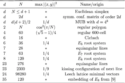
Table 2.1: Known universal optima of N points in real projective spaces RPd-1. The tight simplices are indicated by an asterisk and have maximal squared inner product

(N - d)/(d(N - 1)); for simplicity we omit the Gale duals of the tight simplices.

d N max

I

(x, Y) 2 Name/origin

d N < d + 1 * Euclidean simplex

d 2d * symm. conf. matrix of order 2d

d d(d + 2)/2 1/d MUB with d = 4k

2 N cos2(7r/N) regular polygon

4 60 (v'5 - 1)/4 regular 600-cell 6 16 * Clebsch 6 36 1/4 E6 root system 7 28 * equiangular lines 7 63 1/4 E7 root system 8 120 1/4 E8 root system 23 276 * equiangular lines

23 2300 1/9 kissing configuration of next line

24 98280 1/4 Leech lattice minimal vectors

35 120 * embedding of E8 from [9]

function of squared chordal distance. (See also [13] for context.) This applies in particular to simplices, so all tight simplices are universally optimal.

In fact every known tight code is universally optimal. Moreover, except for the regular 600-cell in S3 and its image in RP3, they all satisfy the design condition just mentioned. For lack of a counterexample, we conjecture that tight codes are always universally optimal. (But see [16] for perspective on why the simplest reason why this might hold fails.)

2.4 Tight codes in RP-l

We now describe what is known about tight codes in real projective spaces. Table 2.1 provides a summary of the current state of knowledge.

Euclidean simplices give the simplest infinite family of tight codes.

Another infinite family of tight simplices comes from conference matrices [40] (see [17,

p. 156]): if a symmetric conference matrix of order 2d exists, then there is a tight simplex of

size 2d in Rd. In particular, we get a tight simplex in Rd whenever 2d - 1 is a prime power congruent to 1 modulo 4. One can also construct such codes through the Weil representation of the group G = PSL2(Fq). Note that the icosahedron arises as the special case q = 5, which is why it is not listed separately in Table 2.1.

Levenshtein [31] described a family of tight codes in RP'- 1 for n a power of 4, based on a construction using Kerdock codes. These codes meet the orthoplex bound (Corollary 5.3 in [17]) and give rise to mutually unbiased bases in their dimensions. The regular 24-cell is the special case with n = 4.

A trivial systematic family of tight codes is formed by the diameters of the regular

polygons in the plane. The remaining configurations in Table 2.1 correspond to exceptional geometric structures.

Table 2.2: Known universal optima of N points in complex projective spaces Cpd-l. The tight simplices are indicated by an asterisk and have maximal squared inner product

(N - d)/(d(N - 1)); for simplicity we omit the Gale duals of the tight simplices as well as

the tight simplices from RPd-1.

d N max I(x, y)12 Name/origin

d 2d * skew-symm. conf. matrix of order 2d

d d2* SIC-POVMs

d d(d

+

1) 1/d MUB with d = pk and p a prime

d 2d

+

1 * skew-Hadamard matrix of order 2d

+

2 (d odd)

d 2d - 1 * skew-Hadamard matrix of order 2d (d even) 4 40 1/3 Eisenstein structure on E8

5 45 1/4 kissing configuration of next line

6 126 1/4 Eisenstein structure on K12

28 4060 1/16 Rudvalis group

SI

1G|

* difference set S in abelian group G

We also observe the phenomenon of Gale duality: tight simplices of size N in KPd-correspond to tight simplices of size N in KPN-d-1. For instance, the Gale dual of the Clebsch configuration gives a tight simplex of 16 points in RP9. See §2.7 for more details.

2.5 Tight codes in

CP'-Table 2.2 lists the tight codes we are aware of in complex projective spaces. For a detailed survey of tight simplices, we refer the reader to Chapter 4 of [28].

Here, we observe a few more infinite families. In particular, if a conference matrix of order 2d exists, then there is a tight code of 2d lines in CPd-1 [44, p. 66]. For prime powers

q = 3 (mod 4), this gives a construction of a tight (q + 1)-point code in CP(q-1)/2. As

mentioned before, such codes may also be constructed using the Weil representation of

PSL2(Fq). Another family of codes of d(d + 1) points in CPd-1, for d an odd prime power, was constructed by Levenshtein [31] using dual BCH codes. These codes meet the orthoplex bound and give rise to mutually unbiased bases in their dimensions. They were rediscovered

by Wootters and Fields [42], with an extension to even characteristic and applications to

physics. A third infinite family is obtained from skew-Hadamard matrices (see [36] for a construction using explicit families of skew-Hadamard matrices and Theorem 4.14 in [28] for the general case).

The most mysterious tight simplices are the awkwardly named SIC-POVMs (symmetric, informationally complete positive operator valued measures). SIC-POVMs are simplices of size d2 in CPd-1, i.e., simplices of the greatest size allowed by Proposition 2.2. These configurations play an important role in quantum information theory, which leads to their name. Numerical experiments suggest they exist in all dimensions, and that they can even be taken to be orbits of the Weyl-Heisenberg group [44, 37]. Exact SIC-POVMs are known for d < 15, as well as d = 19, 24, 35, and 48, and numerical approximations are known for

all d < 67 (see [38]).

Table 2.3: Previously known universal optima of N points in quaternionic and octonionic projective spaces. For simplicity we omit the tight simplices from REp-1 and Cpd-1.

Space N max

I

(x, y)12 Name/origin

Hpd-1 d(2d + 1) 1/d MUB with d = 4k

HIP4 165 1/4 quaternionic reflection group

Op2 819 1/2 _{generalized hexagon of order (2,8)}

[29]). Let G be an abelian group of order N, S a subset of G of order d, and A a natural

number such that every nonzero element of G is a difference of exactly A pairs of elements of S. It follows that d(d - 1) = A(N - 1), and that the vectors

og = (Ws))"sg

give rise to a tight simplex of N points in pd-1 as

X

ranges over all characters of G. As particular cases of this construction, one can obtain a tight simplex of

n

2 + n + 1 points

in CP', when there is a projective plane of order

n.

A generalization of this example was

given in [43], using Singer difference sets, to produce (qd+1l - 1)/(q - 1) points in CPd-1,

with d = (qd - 1)/(q - 1). Similarly, if q is a prime power congruent to 3 modulo 4, then the

quadratic residues give a difference set, yielding a tight simplex of q points in CP(q-3)/2. As another example, there is a difference set of 6 points in Z/31Z (namely, {0, 1, 4, 6, 13, 21}), which gives rise to a tight simplex of 31 points in Cp5.

2.6 Tight codes in HPd-1 and fDhp2

Relatively little is known about tight codes in quaternionic or octonionic projective spaces, aside from the real and complex tight simplices they automatically contain. There is a construction of mutually unbiased bases due to Kantor [27], and two exceptional codes are known.

The 165 points in HP4 from Table 2.3 are constructed using a quaternionic reflection group (Example 9 in [23]). The 819-point universal optimum is a remarkable code in the octonionic projective plane [12]; see also [21] for another construction. It can be thought of as the 196560 Leech lattice minimal vectors modulo the action of the 240 roots of E8 (viewed

as units in the integral octonions), although this does not yield an actual construction: there is no such action because the multiplication is not associative.

2.7 Gale duality

Gale duality is a fundamental symmetry of tight simplices. It goes by several names in the literature, such as coherent duality, Naimark complements, or the theory of eutactic stars. We call it Gale duality because it is a metric version of Gale duality from the theory of

polytopes.

Let K be R, C, or H. Note that Gale duality does not apply to OP2.

Proposition 2.11 (Hadwiger [22]). Let v1, ... , vN span a d-dimensional vector space V