Modeling, analysis and reduction of biological systems

(1)

HAL Id: tel-02169197

https://tel.archives-ouvertes.fr/tel-02169197

Submitted on 1 Jul 2019

HAL is a multi-disciplinary open access archive for the deposit and dissemination of sci-entific research documents, whether they are pub-lished or not. The documents may come from teaching and research institutions in France or abroad, or from public or private research centers.

L’archive ouverte pluridisciplinaire HAL, est destinée au dépôt et à la diffusion de documents scientifiques de niveau recherche, publiés ou non, émanant des établissements d’enseignement et de recherche français ou étrangers, des laboratoires publics ou privés.

Stefano Casagranda

To cite this version:

Stefano Casagranda. Modeling, analysis and reduction of biological systems. Other. Université Côte d’Azur, 2017. English. �NNT : 2017AZUR4049�. �tel-02169197�

(2)

prepared at

Inria Sophia Antipolis - M´

editerran´

ee

and presented at the

Universit´

e Cˆ

ote d’Azur

Graduate School of Information and Communication Sciences

´

Ecole Doctorale STIC

A dissertation submitted in partial fulfillment

of the requirements for the degree of

DOCTOR OF SCIENCE

Specialized in Control, Signal and Image Processing

Modeling, analysis and reduction

of biological systems

Stefano Casagranda

Directed by Jean-Luc Gouz´

e and Delphine Ropers

Defended on June 30th _{2017 in front of the jury composed by:}

Supervisor Jean-Luc Gouzé DR Inria Sophia Antipolis, France Co-Supervisor Delphine Ropers CR Inria Grenoble Rhône Alpes, France Reviewers Riccardo Bellazzi Prof. Università degli Studi di Pavia, Italy

B´eatrice Laroche DR INRA Unit´e MaIAGE Jouy, France Examiners Gregory Batt DR Inria Saclay Ile-de-France, France

Gilles Bernot DR Laboratoire I3S, France Frédéric Dayan Founder ExactCure, France David Rouquié DR Bayer CropScience, France

Invited Eugenio Cinquemani CR Inria Grenoble Rhˆone Alpes, France Suzanne Touzeau CR INRA ISA Sophia Antipolis, France

(3)

(4)

Unit´e de recherche: Inria ´

Equipe: Biocore

Th`

ese de doctorat

Pr´esent´ee en vue de l’obtention du grade de docteur en

Automatique, Traitement du Signal et des Images

de l’Universit´

e Cˆ

ote d’Azur

par

Stefano Casagranda

Mod´

elisation, analyse et r´

eduction

des syst`

emes biologiques

Dirig´

ee par Jean-Luc Gouz´

e et co-encadr´

ee par Delphine Ropers

Soutenue le 30 Juin 2017

Devant le jury compos´e de:

Directeur de thèse Jean-Luc Gouzé DR Inria Sophia Antipolis, France Co-Encadrante de thèse Delphine Ropers CR Inria Grenoble Rhône Alpes, France Rapporteurs Riccardo Bellazzi Prof. Università degli Studi di Pavia, Italie

B´eatrice Laroche DR INRA Unit´e MaIAGE Jouy, France Examinateurs Gregory Batt DR Inria Saclay Ile-de-France, France

Gilles Bernot DR Laboratoire I3S, France Frédéric Dayan Fondateur ExactCure, France David Rouquié DR Bayer CropScience, France

Invit´e Eugenio Cinquemani CR Inria Grenoble Rhˆone Alpes, France Suzanne Touzeau CR INRA ISA Sophia Antipolis, France

(5)

(6)

Abstract

This thesis deals with modeling, analysis and reduction of various biological models, with a focus on gene regulatory networks in the bacterium E. coli. Different mathematical approaches are used. In the first part of the thesis, we model, analyze and reduce, using classical tools, a high-dimensional transcription-translation model of RNA polymerase in E. coli. In the second part, we introduce a novel method called Principal Process Analysis (PPA) that allows the analysis of high-dimensional models, by decomposing them into biologically meaningful processes, whose activity or inactivity is evaluated during the time evolution of the system. Exclusion of processes that are always inactive, and inactive in one or several time windows, allows to reduce the complex dynamics of the model to its core mechanisms. The method is applied to models of circadian clock, endocrine toxicology and signaling pathway; its robustness with respect to variations of the initial conditions and parameter values is also tested. In the third part, we present an ODE model of the gene expression machinery of E. coli cells, whose growth is controlled by an external inducer acting on the synthesis of RNA polymerase. We describe our contribution to the design of the model and analyze with PPA the core mechanisms of the regulatory network. In the last part, we specifically model the response of RNA polymerase to the addition of external inducer and estimate model parameters from single-cell data. We discuss the importance of considering cell-to-cell variability for modeling this process: we show that the mean of single-cell fits represents the observed average data better than an average-cell fit.

(7)

R´

esum´

e (en fran¸cais)

Cette thèse porte sur la modélisation, l’analyse et la réduction de modèles biologiques, notamment de réseaux de régulation génique chez la bactérie E. coli. Différentes ap-proches mathématiques sont utilisées. Dans la 1ère partie de la thèse, on modélise, anal-yse et réduit avec des outils classiques un modèle de transcription-traduction de grande dimension de l’ARN polymérase (RNAP) chez E. coli. Dans la 2de partie, l’introduction d’une nouvelle méthode appelée Analyse de Processus Principaux (PPA) nous permet d’analyser des modèles de haute dimension, en les décomposant en processus biologiques dont l’activité est évaluée pendant l’évolution du système. L’exclusion des processus in-actifs réduit la dynamique du modèle à ses principaux mécanismes. La méthode est appliquée à des modèles d’horloge circadienne, de toxicologie endocrine et de voie de signalisation; on teste également sa robustesse aux variations des conditions initiales et des paramètres. Dans la 3ème partie, on présente un modèle ODE de la machinerie d’expression génique de cellules d’E. coli dont la croissance est contrôlée par un in-ducteur de la synthèse de RNAP. On décrit notre contribution au développement du modèle et analyse par PPA les mécanismes essentiels du réseau de régulation. Dans une dernière partie, on modélise spécifiquement la réponse de RNAP à l’ajout d’inducteur et estime les paramètres du modèle à partir de données de cellules individuelles. On discute l’importance de considérer la variabilité entre cellules pour modéliser ce processus: ainsi, la moyenne des calibrations sur chaque cellule apparaˆıt mieux représenter les données moyennes observées que la calibration de la cellule moyenne.

(8)

R´

esum´

e ´

etendu (en fran¸cais)

La vie est l’un des phénomènes les plus complexes dans l’univers [60]. En ce qui con-cerne la biologie, l’étude d’une seule unité de vie, la cellule, est une tâche infiniment compliquée.

Au cours du siècle dernier, les mécanismes cellulaires ont été étudiés dans différentes per-spectives par des biologistes, des mathématiciens, des ingénieurs: par des expérimentations dans différentes conditions, par la modélisation mathématique du comportement cellu-laire, par la calibration de ces modèles en utilisant des données expérimentales, par l’analyse et la réduction des structures de ces modèles à des fins différentes.

Toutes ces différentes études ont créé un domaine, un grand ensemble de connaissances, appelé biologie des systèmes [58], où différents auteurs ont contribué dans des directions diverses. L’objectif de cette thèse est d’y ajouter une brique.

Motivations

Un sujet majeur de la biologie des systèmes est la modélisation et l’analyse des réseaux cellulaires.

La création de modèles biologiques et leurs simulations dans différentes conditions sont déterminantes pour comprendre comment l’adaptation des organismes vivants aux sig-naux environnementaux résulte de grands réseaux de métabolites, d’ARN, de protéines et de leurs interactions mutuelles.

De plus en plus grands modèles cinétiques de réseaux cellulaires sont aujourd’hui publiés, comme résultat de décennies de travail en biologie, de progrès récents dans les bio-technologies [26, 60] et des progrès dans la modélisation et les approches d’estimation de paramètres (par exemple, voir [23] et [64]). La grande taille de ces modèles et leur non linéarité (en raison de boucles de rétroaction complexes) rendent leur calibration et leur analyse dynamique plutôt difficiles. Plus précisément, il est extrêmement difficile de relier le comportement global du système au fonctionnement de processus cellulaires spécifiques (par example La transcription de l’ARN, la phosphorylation des protéines

(9)

ou la formation de complexes), alors que ce gain de connaissances est essentiel pour identifier quels sont les processus cellulaires cl´es pour l’adaptation environnementale et quand ils sont en jeu.

Dans cet esprit, notre travail aborde différentes fa¸cons d’obtenir des informations sur le fonctionnement des cellules, en particulier sur la bactérie Escherichia coli [6]. Le réseau de régulation des gènes et la croissance de cet organisme modèle sont une grande source d’intérêts pour la communauté scientifique et pour l’industrie. En outre, l’expérimentation et la modélisation de E. coli sont l’un des principaux intérêts de l’équipe Inria Ibis et du groupe de Hans Geiselmann à l’Univ. Grenoble-Alpes avec lequel j’ai collaboré.

Approche

Les méthodes de réduction jouent un rôle central dans la conception des modèles. La description de la synthèse et de la consommation des composants biologiques d’un réseau peut conduire à un gros ensemble d’équations différentielles ordinaires (ODE): les ap-proches de modèles classiques comme des equilibrium approximation ou des quasi-steady-state approximation (QSSA) [103] aident à réduire la dimension du modèle, à travers la séparation des échelles de temps. Cependant, la réduction du modèle avec ces approches n’est pas une tâche facile, en particulier pour les systèmes avec des boucles de rétroaction, que l’on trouve souvent dans les systèmes biologiques. Pour cette raison, dans la première partie de la thèse, nous montrons la réduction d’un modèle ODE de grande dimension, décrivant l’activité de l’ARN polymérase dans E. coli, qui favorise sa propre transcription. En utilisant la théorie des systèmes monotones et les arguments d’échelles de temps, nous pouvons le réduire à un modèle avec deux variables (ARN polymérase et son ARNm). Nous analysons le modèle réduit, en particulier la relation entre le taux de production RNAP, la quantité de ribosome et le taux de croissance cellulaire.

Ces outils classiques ont permis le développement de modèles plus grands, dont les formes réduites conservent encore de nombreuses équations et boucles de rétroaction. Si l’on considère le mécanisme complet d’expression de gènes de E. coli, par exemple, il ne

(10)

comprend pas seulement l’ARN polymérase, mais aussi les ribosomes, les protéines cellu-laires et les métabolites, ainsi que leurs interactions régulatrices mutuelles. Pour analyser ces modèles cellulaires complexes, dans la deuxième partie de la thèse, nous présentons une nouvelle approche numérique appelée Analyse de Processus Principaux (PPA) qui permet à la fois l’analyse et la réduction des systèmes biologiques sans modifier leur structure principale. Basé sur la décomposition de la dynamique du système en proces-sus biologiques actifs ou inactifs par rapport à une certaine valeur seuil, PPA apporte la connaissance des processus clés impliqués lors de l’évolution du système dans différentes fenêtres temporelles. Dans chaque fenêtre temporelle, le système est réduit à ses princi-paux mécanismes, négligeant les processus biologiques considérés comme étant inactifs. Cette approche est une méthode simple à utiliser, qui constitue un outil supplémentaire et utile pour analyser le comportement dynamique complexe des systèmes biologiques. La réduction de modèle qui en résulte n’entraˆıne pas une perte d’information ou de changements significatifs de la structure du modèle, comme cela se produit avec d’autres techniques de réduction. Pour tester la qualité de notre approche, nous appliquons la PPA sur différents systèmes biologiques à grande dimension: modèles d’horloges cir-cadiennes, toxicologiques, et de voies de signalisation. Chaque analyse donne des in-formations biologiques importantes et, pour la plupart, nous obtenons un sous-modèle pour chaque fenêtre de temps proposée. En fait, la PPA peut être appliqué à n’importe quel modèle biologique exprimé par ODEs et il a été récemment utilisé par d’autres équipes de recherche [88,95] à des fins d’analyse et de réduction, obtenant des résultats intéressants. Parce que notre approche est basée sur la connaissance a priori des trajec-toires du système, elle dépend des paramètres et des valeurs de condition initiale: nous avons également testé la robustesse de la PPA aux valeurs des paramètres en utilisant l’analyse de sensibilité globale et les valeurs de condition initiale à l’aide d’une méthode ayant des similitudes avec un formalisme piece-wise linear.

Après avoir testé notre technique sur différents modèles biologiques, dans la troisième partie de la thèse, nous l’appliquons pour l’analyse d’un modèle, con¸cu par Delphine Ropers de l’équipe Inria Ibis, qui décrit le fonctionnement du mécanisme d’expression des gènes. En tant que tel, le modèle étend avec d’autres modules le modèle de transcription-traduction de l’ARN polymérase décrite dans la première partie. Il est également capable

(11)

de décrire le contrôle externe de la croissance de E. coli par un inducteur externe (IPTG) agissant sur la transcription des ARNm de la sous-unité de l’ARN polymérase.

La dernière partie de la thèse étudie en outre le contrôle externe de E. coli par IPTG, au moyen d’un modèle beaucoup plus simple de ce système, axé sur les processus clés nécessaires pour reproduire des observations biologiques sur l’expression des gènes dans des cellules individuelles, avec ou sans IPTG. Ce système est l’occasion d’aborder le problème de l’estimation des paramètres, qui suit immédiatement celui de la réduction du modèle. Dans le cas présent, nous calibrons le modèle simple en utilisant des données de gènes rapporteurs et des données de croissance obtenues dans des cellules individuelles traitées ou non avec IPTG [51]. Nous montrons que la calibration du modèle sur chaque cellule est préférable à la calibration d’un modèle moyen aux données moyennes, en raison de la grande variabilité entre les cellules et bien que cette variabilité soit incluse dans la procédure de calibration comme une erreur de mesure.

Organisation du manuscrit et contributions

Le manuscrit est organisé comme suit. Dans le premier chapitre introductif, nous décrivons brièvement la biologie cellulaire de E. coli et des méthodes pour contrôler sa croissance (Chapitre 3). Dans le deuxième chapitre introductif, nous présentons différents formalismes classiques pour concevoir, analyser et réduire les systèmes de réseau de régulation des gènes (GNR) (Chapitre4).

Dans le Chapitre 5, nous nous concentrons sur le modèle de transcription-traduction de l’ARN polymérase dans E. coli. Mes contributions sont: effectuer des simulations de modèles complets et réduits avec un nouvel ensemble de paramètres pour obtenir des résultats plus réalistes d’un point de vue biologique; comparer un modèle classique de polymérase RNAP au modèle réduit obtenu, y compris une étude de sensibilité par rapport au nombre de ribosomes; concevoir et étudier un système réduit incluant un taux de croissance variable. Une version de ce chapitre a été soumise au journal Bulletin of Mathematical Biology, dans lequel je suis le deuxième auteur.

(12)

Dans le Chapitre 6, nous présentons l’analyse de processus principaux et la notion de poids relatif associés aux processus afin de les comparer. Nous appliquons la PPA à un modèle de rythmes circadiens chez les mammifères [73]: les erreurs relatives globales sont utilisées pour tester la qualité de la réduction, tandis que l’application de l’analyse de sensibilité globale nous permet de tester l’influence des paramètres du modèle sur ces erreurs. Les résultats obtenus prouvent la robustesse de notre méthode. J’ai développé en détail cette approche numérique à partir d’une version préliminaire développée par Jean-Luc Gouzé, avec la collaboration de ma co-encadrante Delphine Ropers. J’ai ef-fectué l’analyse de sensibilité globale avec l’aide de Suzanne Touzeau (Biocore et INRA). Une version en papier de journal de ce chapitre a été soumise à Journal of Theoretical Biology dans laquelle je suis le premier auteur.

Les premières applications de PPA sur un modèle circadien de Drosophila [72] et un modèle de voie de signalisation [68] sont présentés en AnnexeB: nous ne les insérons pas dans un chapitre ordinaire pour éviter les redondances avec le Chapitre 6. Ce travail a été présenté au 23ème Méditerranée Conférence sur le contrôle et l’automatisation MED, tenue à Torremolinos, en Espagne, du 16 au 19 juin 2015 (avec des relectures par des pairs) et a été accepté comme un papier de conférence dans lequel je suis le premier auteur.

Le Chapitre7traite de la robustesse du modèle aux conditions initiales: nous évaluons la qualité de la PPA sur un ensemble de valeurs initiales possibles. Par souci de simplicité, et parce que les ordres de grandeur peuvent être importants dans les modèles biologiques, nous considérons les conditions initiales dans les rectangles représentant un ordre de grandeur et nous limitons cette approche à la dimension deux. Le plan est divisé en une grille logarithmique et nous appliquons (sous certaines hypothèses concernant la monotonie des processus) la PPA en calculant une limite maximale pour les poids de chaque processus. Nous conservons les processus actifs qui ont un poids dynamique plus élevé qu’un seuil fixe. Avec ce travail, nous démontrons la robustesse de notre méthode aux variations des conditions initiales. J’ai effectué ce travail en collaboration avec mon directeur de thèse Jean-Luc Gouzé et il sera présenté au Congrès mondial IFAC 2017

(13)

(avec relectures par les pairs) et a été accepté comme un papier de conférence dans lequel je suis le premier auteur.

Dans le Chapitre8, nous appliquons la PPA sur un modèle déterministe con¸cu par Bayer CropScience [79], qui décrit les effets toxicologiques d’un fongicide sur les souris mâles. Nous voulons vérifier si les processus du modèle calibré sont actifs dans l’ordre attendu, connaissant la série d’événements clés proposés pour cette substance [96]. Pour cela, nous utilisons, en tant que critère de comparaison, les valeurs absolues des modèles bi-ologiques et un seuil variable qui dépend des valeurs maximales et minimales des proces-sus dans chaque variable. Nous appelons cette approche l’Analyse Absolue des Procesproces-sus Principaux (APPA). Le travail a été réalisé en collaboration avec David Rouquié, senior researcher au centre de recherche en toxicologie de Bayer CropScience et avec Frédéric Dayan, fondateur d’ExactCure et ancien chef d’équipe de R&D chez Dassault Systèmes. Le système a été modélisé en 2014 par un stagiaire Bayer CropScience, Benjamin Mi-raglio, sous la supervision de David Rouquié et Frédéric Dayan. Ce travail fera partie d’un article de journal futur.

Après avoir établi PPA et testé la méthode sur différents modèles, nous l’utilisons main-tenant pour étudier un nouveau modèle mathématique dans E. coli. Le modèle a été con¸cu par ma co-encadrante Delphine Ropers et décrit les mécanismes d’expression des gènes de la bactérie dans les détails ainsi que l’effet de l’inducteur IPTG sur celui-ci. Dans le Chapitre 9 nous présentons notre contribution au développement du modèle pour la description du taux de croissance cellulaire. Nous appliquons ensuite une PPA sur le modèle GEM pour analyser ses mécanismes de base et nous étudions l’effet de l’addition d’IPTG au milieu de culture sur la croissance de la bactérie. Ce travail fera partie d’un article de journal futur.

Dans le Chapitre 10 nous poursuivons l’étude du contrôle externe de E. coli par IPTG avec un modèle plus simple calibré avec des données expérimentales de surface cellulaire et de fluorescence, obtenu par Jérôme Izard lors de sa thèse de doctorat dans le labo-ratoire Adaptation et Pathogénie des Micro-organismes (Univ. Grenoble-Alpes). Nous comparons la calibration sur chaque cellule individuelle et la calibration de la cellule moyenne et montrons comment adapter le modèle à chaque cellule individuelle au lieu

(14)

d’une cellule moyenne, permettant d’obtenir plus d’informations sur la variabilité entre les cellules et donnant une meilleure qualité de calibration. J’ai effectué cette analyse en collaboration avec Eugenio Cinquemani de l’équipe Ibis et Delphine Ropers. Ce travail fera partie d’un article de journal futur.

Les conclusions de ces travaux de recherche ainsi que les perspectives sont donn´ees au Chapitre11.

(15)

Cette thèse a été dirigée par Jean-Luc Gouzé (Inria Biocore) et co-encadrée par Delphine Ropers (Inria Ibis). Elle a bénéficié du support financier du Conseil Régional PACA et du projet RESET (ANR-11-BINF-0005) du programme Investissements d’Avenir Bio-informatique.

(16)

First of all I want to thank my supervisor Jean-Luc Gouzé to have picked me to be part of his team three and a half years ago: I have a lot of great memories about all the discussions we have done together about science in your office and I will always thank you for all the opportunities you gave me to learn more and more at Inria and around the world. It was a big pleasure to work with you. A big thanks goes to my co-supervisor Delphine Ropers: you have dedicated so much time to my scientific and professional growth. I will always remember the days in the laboratory in Grenoble when you “transformed” me into a biologist, performing real experiments on E. coli : since that week we had a really strong collaboration together and I will always carry these memories with me. A very special gratitude goes to Eugenio Cinquemani and Suzanne Touzeau: it was a pleasure to have worked with you and to have shared this experience with people so strong in science as you. You have taught me a lot. I am grateful to Hidde de Jong who introduced me in the RESET project. It was an honor to have been a part of your meetings in Grenoble: I have always admired your humility and kindness in listening to others, despite your large scientific knowledge. Special thanks go to Riccardo Bellazzi, Béatrice Laroche, Frédéric Dayan, David Rouquié, Gregory Batt and Gilles Bernot to have taken the time to read my work and to be here today. Thanks to my friends (and colleagues) Nicolas, Francesco, Pierre-Olivier, Natacha, David, Alfonso, Elsa, Camille, Riccardo, Lucie, Ivan, Carlos, Melaine, Ignacio, Ismail, Diego, Marjorie, Eleni, Claudia, Quentin, Sofia, Bapan and the babyfoot for the wonderful time spent together inside and outside Inria! Merci beaucoup to Stephanie to have helped me all these years with my missions and my continuous requests! Thanks to Olivier, Frédéric, Madalena, Francis, Marie-Line for having always made me feel very comfortable in the Biocore team. Un grazie gigante a Marco: I remember the day you came in my office looking for Italians! Since that day a wonderful friendship started: thank you for everything, I won’t never forget it. A big efharistò to my best porcellini Christos and Konstantinos: you are great and kind people and you make me really understand that “una faccia una razza” and that team Porco Rosso is just the best. Grazie Lamberto for all the good talks at Inria: it was a pleasure meeting you, even for a short time! Thanks also to other great people I

(17)

met at Inria, namely Dmitry, Matthias, Adam, Dora, Nathalie, Valeria, David, Laurent and Juliette. Il ringraziamento più grande di tutti va a te, Susi, per tutto il sostegno che mi hai dato in questi mesi e per tutte le bellissime emozioni che mi fai provare: sei una persona meravigliosa, piena di passione per la vita e di energie inesauribili. Sei una fiamma vivacissima dalle mille sfumature e sono onorato di poter condivere tanto assieme a te! Grazie a voi mamma e papà per tutti gli aiuti che mi avete dato in questi anni e per avere sempre creduto in me e in quello che faccio! Un grazie anche a Franca per essere stata sempre gentile e ospitale con me. Grazie agli amici che ci sono e che c’erano nella nostra Nizza: a Matteo, Pietro, Massimo, Marta, Greta, Andrea, Massimo, Andrea, Enrico, Laura e Giulia. Due coincidenze fortunate al karaoke dell’Akathor e davanti alla porta sul retro del Tapaloca hanno portato ad una vita di bellissimi momenti che non dimenticherò mai. Grazie agli amici di Pavia: al mio dude Luca, a Marco, Giò, Sandro, Amer, Izio, Rassa, Ruffo, Cisco, Rich, Paul, Antonio, Federico, Ferro, Duca e Pelle. Ogni volta che ritorno mi sento sempre uno di voi e sembra che il tempo non stia volando affatto.

(18)

Abstract iii Acknowledgements xiii Contents xv 1 Introduction 1 1.1 Motivations . . . 1 1.2 Approach . . . 2

1.3 Organization of the manuscript and contributions . . . 3

2 Introduction (en fran¸cais) 7 3 Notes on molecular cell biology 9 3.1 Escherichia coli . . . 9 3.2 Growth of E. coli . . . 10 3.3 Gene expression. . . 12 3.3.1 Transcription . . . 13 3.3.2 Translation . . . 14 3.3.3 mRNA degradation . . . 15

3.4 Regulation of gene expression in E. coli . . . 16

4 Modeling genetic regulatory network systems 19 4.1 Ordinary differential equation models . . . 20

4.1.1 Modeling transcription-translation . . . 20

4.1.2 Quasi-steady-state assumption of mRNA concentration . . . 23

4.2 Analysis of a genetic bistable switch . . . 24

4.2.1 Phase plane analysis . . . 24

4.2.2 Jacobian matrix . . . 26

4.2.3 Piece-wise affine linear system . . . 27

4.3 Parameter sensitivity analysis . . . 29

4.3.1 Local sensitivity analysis . . . 30

4.3.2 Global sensitivity analysis . . . 31

4.4 Parameter fitting . . . 33

5 Reduction and stability analysis of a transcription-translation model of RNA polymerase 35 5.1 Introduction. . . 36

(19)

5.2 The coupled transcription-translation model of RNA polymerase . . . 37

5.2.1 Description of the model. . . 37

5.2.2 Full equation . . . 38

5.3 Time-scale reduction (fast-slow behavior) . . . 40

5.3.1 Parameter values for the coupled transcription-translation models of RNA polymerase . . . 40

5.3.2 Separation of the full system into “fast” and “slow” variables . . . 41

5.4 Verification of the applicability of the Tikhonov’s theorem for the fast subsystems . . . 44

5.5 Application of the Tikhonov’s theorem . . . 46

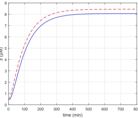
5.6 Dynamical study of the reduced system . . . 48

5.6.1 Simulations of the full and the reduced system . . . 48

5.6.2 Equilibria of the reduced system . . . 48

5.6.3 Stability of equilibria. . . 49

5.7 Applications to other models . . . 51

5.8 Comparison with a classical model of RNA polymerase . . . 52

5.9 System with a variable growth rate . . . 54

5.10 Conclusion . . . 56

6 Principal process analysis and its robustness to parameter changes 59 6.1 Introduction. . . 60

6.2 Methodology . . . 62

6.2.1 Principal process analysis (PPA) . . . 62

6.2.2 Visualization of process activities . . . 64

6.2.3 First model reduction . . . 65

6.2.4 Creation of chains of sub-models . . . 67

6.2.5 Global sensitivity analysis . . . 68

6.3 Model description. . . 69

6.4 Principal process analysis and first reduction . . . 70

6.5 Creation of sub-models. . . 73

6.6 Parameter influence . . . 79

7 Principal process analysis and reduction of biological models with dif-ferent orders of magnitude 85 7.1 Introduction. . . 85

7.2.1 Principal process analysis and model reduction . . . 86

7.2.2 Principal process analysis and model reduction based on initial conditions in a rectangle . . . 88

7.2.3 Possible transitions between domains. . . 90

7.3 The gene expression model . . . 92

7.4 Model reduction from an initial condition . . . 93

7.5 Model reduction in a rectangle . . . 95

7.6 Conclusion . . . 98 8 Principal process analysis applied to a model of endocrine toxicity

(20)

8.1 Introduction. . . 101

8.2.1 Absolute principal process analysis . . . 103

8.2.2 Visualization of the process activity . . . 104

8.3 Hierarchical graph . . . 105 8.4 Model . . . 106 8.4.1 Blood compartment . . . 106 8.4.2 Liver compartment . . . 106 8.4.3 Brain compartment . . . 109 8.4.4 Thyroid compartment . . . 109 8.4.5 The data . . . 110

8.4.6 Different experiments in silico . . . 110

8.5 Absolute principal process analysis on the experiment 1A . . . 115

8.6 Absolute principal process analysis on the experiment 2B . . . 116

8.7 Conclusion and future steps . . . 121

9 Model and control of the gene expression machinery in E. coli 123 9.1 Introduction. . . 123

9.2 The model. . . 125

9.2.1 Growth rate. . . 128

9.3 The effect of IPTG on E. coli growth. . . 130

9.4 Model analysis with three-level PPA . . . 132

9.4.1 Methodology . . . 132

9.4.2 Different applications . . . 135

9.4.2.1 Nutrient stress condition . . . 135

9.4.2.2 IPTG stress condition . . . 140

10 Single-cell model calibration of growth control experiments in E. coli147 10.1 Introduction. . . 147

10.2 Model . . . 149

10.3.1 Data . . . 152

10.3.2 Extraction of cellular profiles . . . 152

10.3.3 Calculation of average cell profiles . . . 155

10.3.4 Calibration of the model . . . 156

10.4 Results. . . 157

10.4.1 Cellular profiles . . . 157

10.4.2 Calibration of the average cell model . . . 157

10.4.3 Calibration of the single-cell models . . . 158

10.4.4 Comparison . . . 159

11 Conclusion and perspectives 165 11.1 Classical tools for the analysis and reduction of biological models . . . 165

11.2 New tools for the analysis and reduction of biological systems . . . 166

(21)

11.4 Single-cell and average cell calibration of the gene expression machinery

control in E. coli . . . 168

12 Conclusion et perspectives (en fran¸cais) 171 12.1 Outils classiques pour l’analyse et la r´eduction des mod`eles biologiques . . 171

12.2 Nouveaux outils pour l’analyse et la réduction des systèmes biologiques . 172 12.3 Modélisation et analyse du mécanisme d’expression des gènes dans E. coli 174 12.4 Calibration d’un modèle de contrôle de la machinerie d’expression des gènes dans E. coli en utilisant les profils de la cellule individuelle et la moyenne . . . 175

A List of publications 177 B First application of principal process analysis on biological models 179 B.1 Methodology . . . 180

B.1.1 Principal process analysis (PPA) . . . 180

B.1.2 Visualization of process activities . . . 182

B.1.3 First model reduction . . . 183

B.1.4 Creation of chains of sub-models . . . 184

B.2 Model for circadian rhythms in Drosophila. . . 185

B.2.1 Description . . . 185

B.2.2 Model reduction . . . 186

B.2.3 Qualitative tool: heat process map . . . 187

B.2.4 Creation of sub-models based on time windows . . . 189

B.3 Model for the influence of RKIP on the ERK signaling pathway . . . 192

B.3.1 Description . . . 192

B.3.2 Model reduction . . . 193

B.3.3 Qualitative tool: 3-D process map . . . 193

B.4 Conclusions . . . 195

B.5 Supplementary materials. . . 195

C Supplementary materials of Chapter 5 199 C.1 Monotone systems . . . 199

C.2 Tikhonov’s theorem . . . 200

D Supplementary materials of Chapter 6 201 D.1 Full mammalian model. . . 201

D.2 Switching times . . . 204

D.3 Neglected procceses. . . 204

D.3.1 First reduced model . . . 204

D.3.2 Second reduced model: sub-models . . . 204

D.4 Dynamical process maps . . . 205

E Supplementary materials of Chapter 8 209 E.1 Full dynamics of the experiments 1A, 2A, 2B . . . 209

(22)

F.1 Parameters and initial values of the GEM model . . . 213

G Supplementary materials of Chapter 10 217

G.1 Model parameters for each c calibration . . . 217

(23)

(24)

Introduction

Life is one of the most complex phenomena in the universe [60]. When it comes to biology, the study of even a single unit of life, the cell, is not at all an easy task. In the last century, cellular mechanisms were studied from different perspectives by biologists, mathematicians, engineers: through experimentations in different conditions, mathematical modeling of cell behavior, calibration of these models using experimental data, analysis and reduction of model structures for different purposes.

All these different studies created a field, a big wall of knowledge, called systems biology [58], where different minds contributed in their own way.

The aim of this thesis is to add a brick to it.

1.1 Motivations

A major topic of systems biology is in fact the modeling and analysis of cellular networks. The creation of biological models and their simulations in different conditions are de-terminant in understanding how adaptation of living organisms to environmental cues results from large networks of metabolites, RNAs, proteins, and their mutual interac-tions.

Larger and larger kinetic models of cellular networks are nowadays published, as a results of decades of work in biology, recent advances in high throughput technologies [26,60] and progress in modeling and parameter estimation approaches (for example, see [23] and [64]). The large size of these models and their non linearity due to complex feedback loops make their calibration and dynamical analysis rather difficult. More specifically,

(25)

it is extremely difficult to relate the global behavior of the system to the functioning of specific cellular processes (e.g. RNA transcription, protein phosphorylation, or complex formation), while this gain of knowledge is crucial to identify what are the key cellular processes for the environmental adaptation and when they are at play.

In this spirit, our work addresses different ways to gain information on cell functioning, especially on the bacterium Escherichia coli [6]. The gene regulatory network and the growth of this model organism is a source of interest in the scientific community and industry. Furthermore experimental and modeling of E. coli are one of the main interest of the Inria Ibis team and of the group of Hans Geiselmann at the Univ. Grenoble-Alpes with which I collaborated.

1.2 Approach

Reduction methods play a pivotal role in model designing. Describing the synthesis and the consumption of the biological components of a network can lead to a large set of ordinary differential equations (ODEs): classical model approaches as quasi-equilibrium approximations or quasi-steady-state approximations (QSSA) [103] help to reduce con-sistently the model dimension, through time scale separation. However model reduction with these approaches is not an easy task, in particular for systems with feedback loops, as often found in biological systems. For this reason, in the first part of the thesis, we show the reduction of a high dimensional ODE model, describing the activity of RNA Polymerase in E. coli, which promotes its own transcription. Using monotone system theory and time-scale arguments we are able to reduce it to a model with two variables (RNA polymerase and its mRNA). We analyze the reduced model with a specific fo-cus on the relation between the RNAP production rate, ribosome quantity and cellular growth rate.

These classical tools have allowed the development of larger models, whose reduced forms still retain many equations and feedback loops. If we consider the full gene expression machinery of E.coli, for instance, it does not only include the RNA polymerase, but also the ribosomes, cell proteins and metabolites, as well as their mutual regulatory interac-tions. For analyzing such complex cellular models, in the second part of the thesis, we present a new numerical approach called Principal Process Analysis (PPA) that allows both the analysis and the reduction of biological systems without changing their main structure. Based on the decomposition of the system dynamics into biological processes that are active or inactive with respect to a certain threshold value, PPA brings the knowledge of which are the key processes involved during the system evolution in differ-ent time windows. In each time window the system is reduced at its core mechanisms,

(26)

neglecting the biological processes that are considered to be inactive. This approach is a simple-to-use method, which constitutes an additional and useful tool for analyzing the complex dynamical behavior of biological systems. The resulting model reduction does not lead to a loss of information or significantly changes of the model structure as can happen with other reduction techniques. To test the quality of our approach, we apply PPA on different high dimensional biological systems: circadian clocks, toxicological and signaling pathway models. Each analysis gives important biological information and for most of them we obtain a sub-model for each proposed time window. In fact PPA can be applied to any biological model expressed by ODEs and it has been recently used by other research teams [88,95] for analysis and reduction purposes, obtaining interesting results. Because our approach is based on the a priori knowledge of system trajectories, it depends on parameter and initial condition values: we have also tested the robustness of PPA to parameter values using global sensitivity analysis and to initial condition values using a method, which shares similarity with piece-wise linear formalism. After having tested our technique on different biological models, in the third part of the thesis, we apply it to analyze a model, designed by Delphine Ropers from the Inria Ibis team, that describes the functioning of the gene expression machinery. As such, the model extends with other modules the transcription-translation model of RNA poly-merase described in the first part. It is also able to describe the external control of the growth of E. coli through an external inducer (IPTG) acting on the transcription of RNA polymerase subunit mRNAs.

The last part of the thesis further studies the external control of E. coli growth by IPTG, by means of a much simpler model of this system, centered around the key processes needed to reproduce biological observations on gene expression in single cells, with or without IPTG. This system is an occasion to tackle the problem of parameter estimation, which immediately follows that of model reduction. In the present case, we calibrate the simple model using reporter gene data and growth data obtained in single cells treated or not with IPTG [51]. We show that single-cell calibration of the model is preferable over fitting a mean model to the average data, due to the large cell-to-cell variability and despite its inclusion into the calibration procedure as a measurement error.

1.3 Organization of the manuscript and contributions

The manuscript is organized as follows. In the first introductory chapter we describe in a nutshell the cell biology of E. coli and methods to control its growth (Chapter 3). In the second introductory chapter we present different classical formalisms to design, analyze and reduce gene regulatory network (GNR) systems (Chapter 4).

(27)

In Chapter 5 we focus on the transcription-translation model of RNA polymerase in E. coli. My contributions are: performing simulations of the full and reduced models with a new set of parameters to have more realistic results from a biological point of view; comparing a classical model of RNA polymerase to the reduced model obtained, including a sensitivity study with respect to the number of ribosomes; designing and studying a reduced system including a variable growth rate. A version of this chapter has been submitted to the journal Bulletin of Mathematical Biology, in which I am second author.

In Chapter6 we introduce principal process analysis and the notion of relative weights associated with processes in order to compare them. We apply PPA to a model of circadian rhythms in mammals [73]: global relative errors are used to test the quality of the reduction, while applying global sensitivity analysis allows us to test the influence of the model parameters on these errors. The results obtained prove the robustness of our method. I developed in detail this numerical approach from a preliminary version developed by Jean-Luc Gouz´e, with the collaboration of my co-supervisor Delphine Ropers. I performed the global sensitivity analysis with the help of Suzanne Touzeau. A journal paper version of this chapter has been submitted to Journal of Theoretical Biology in which I am first author.

The first applications of PPA on a Drosophila Circadian model [72] and a signaling pathway model [68] are presented in Appendix B: we do not insert them in a regular chapter to avoid redundancy with Chapter 6. This work has been presented at the 23rd Mediterranean Conference on Control and Automation MED, held in Torremolinos, Spain, on June 16th-19th, 2015 (with peer reviewed proceedings) and has been accepted as a conference paper in which I am first author.

Chapter7deals with the model robustness to the initial conditions: we assess the quality of PPA on an entire set of possible initial values. For the sake of simplicity, and because the orders of magnitude can be large in biological models, we consider initial conditions in rectangles representing one order of magnitude and we limit this approach to dimension two. The plane is divided in a logarithmic grid and we apply (under some assumptions concerning the monotonicity of the processes) PPA by computing a maximal bound for the weights of of each process. We retain the active processes that have a dynamical weight higher that a fixed threshold. With this work we prove the robustness of our method to variations of initial conditions. I performed this work in collaboration with my supervisor Jean-Luc Gouz´e and it will be presented at the IFAC 2017 World Congress (with peer reviewed proceedings) and has been accepted as a conference paper in which I am first author.

(28)

In Chapter 8 we apply PPA on a deterministic model designed by Bayer CropScience [79], that mimics the toxicological effects of a fungicide on male mice. We want to verify if the processes of the calibrated model get active in the order expected, knowing the series of key events that have been proposed for this substance [96]. For this purpose we use, as a comparison criteria, the absolute values of the biological models and a varying threshold that depends on the maximum and minimum values of the processes in each variable. We call this approach Absolute Principal Process Analysis (APPA). The work has been done in collaboration with David Rouquié, senior researcher at the toxicology research center of Bayer CropScience, and with Frédéric Dayan, ExactCure founder and former R&D team leader at Dassault Systèmes. The system was modeled in 2014 by a Bayer CropScience intern, Benjamin Miraglio, under the supervision of David Rouquié and Frédéric Dayan. This work will be a part of a future journal paper.

Having established PPA and tested the method on various models, we now use it to study a new mathematical model in E. coli. The model has designed by my co-supervisor Delphine Ropers and describes the gene expression machinery of the bacterium in details as well has the effect of the inducer IPTG on it. In Chapter9we present our contribution to the model development for the description of cell growth rate. We then apply PPA on the GEM model to analyze its core mechanisms and we study the effect of IPTG addition to the culture medium on the bacterium growth. This work will be a part of a future journal paper.

In Chapter10 we continue the study of the external control of E. coli by IPTG with a simpler model calibrated with experimental data of cellular area and fluorescence, ob-tained by Jérôme Izard during his PhD thesis in the laboratoire Adaptation et Pathogénie des Micro-organismes (Univ. Grenoble-Alpes). We compare single-cell calibration and average-cell calibrations, and show how fitting the model to each individual cell instead of an average cell, leads to more information about cell-to-cell variability and results in a better calibration quality. I performed this analysis in collaboration with Eugenio Cinquemani from the Ibis team and Delphine Ropers. This work will be a part of a future journal paper.

(29)

(30)

Introduction (en fran¸cais)

Cette thèse porte sur la modélisation, l’analyse et la réduction de modèles biologiques, notamment de réseaux de régulation génique chez la bactérie E. coli. Différentes ap-proches mathématiques sont utilisées. Dans la 1ère partie de la thèse, on modélise, anal-yse et réduit avec des outils classiques un modèle de transcription-traduction de grande dimension de l’ARN polymérase (RNAP) chez E. coli. Dans la 2de partie, l’introduction d’une nouvelle méthode appelée Analyse de Processus Principaux (PPA) nous permet d’analyser des modèles de haute dimension, en les décomposant en processus biologiques dont l’activité est évaluée pendant l’évolution du système. L’exclusion des processus in-actifs réduit la dynamique du modèle à ses principaux mécanismes. La méthode est appliquée à des modèles d’horloge circadienne, de toxicologie endocrine et de voie de signalisation; on teste également sa robustesse aux variations des conditions initiales et des paramètres. Dans la 3ème partie, on présente un modèle ODE de la machinerie d’expression génique de cellules d’E. coli dont la croissance est contrôlée par un in-ducteur de la synthèse de RNAP. On décrit notre contribution au développement du modèle et analyse par PPA les mécanismes essentiels du réseau de régulation. Dans une dernière partie, on modélise spécifiquement la réponse de RNAP à l’ajout d’inducteur et estime les paramètres du modèle à partir de données de cellules individuelles. On discute l’importance de considérer la variabilité entre cellules pour modéliser ce processus: ainsi, la moyenne des calibrations sur chaque cellule apparaˆıt mieux représenter les données moyennes observées que la calibration de la cellule moyenne.

(31)

(32)

Notes on molecular cell biology

Various biological systems have been studied during this PhD thesis, from the bacterium Escherichia coli to the fly Drosophila. Rather than describing these systems in detail, we will introduce in this chapter important concepts of cell biology in the case of the bacterium E. coli. For more details, see [6] and [7].

3.1 Escherichia coli

Because cells descend from a common ancestor, studying properties of one organism can help to understand the properties of others [6]: usually these model organisms are chosen for their easy genetic manipulation and cultivation in the laboratory or because they can survive under certain conditions of stress.

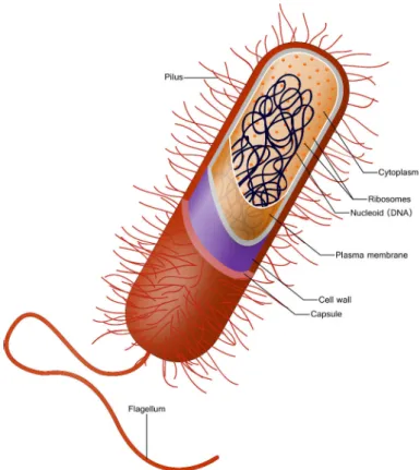
The bacterium Escherichia coli is a model organism for prokaryotic cells. It is com-monly found in the lower intestine of warm-blooded organisms and was one of the first organisms to have its complete genome sequenced [25]. The bacterium has a rod-shaped form and is typically 2 µM long. Its cell wall consists of an outer membrane and an inner membrane containing only one compartment with cytoplasm and generally, no organelles. The cytoplasm contains most of the cell components: DNA, RNAs, proteins, metabolites... It is the place where most cellular processes take place: the metabolism, DNA replication, gene expression processes for instance (see Figure3.1). Complex molec-ular machineries also present in the cytoplasm catalyze these processes: for instance, the ribosomes, responsible for the production of proteins, and the RNA polymerase, involved in RNA synthesis.

(33)

Figure 3.1: Schematic representation of a prokaryotic cell. Intracellular com-ponents (proteins, DNA and metabolites) are located within the cytoplasm, protected by the cell wall composed of two membranes. On their surface, E. coli cells carry a lash-like appendage called flagellum, useful to move in a fluid-like environment and to

detect concentration gradients and other signals (picture taken from [1]).

3.2 Growth of E. coli

E. coli reproduce asexually by a process called binary fission [84], involving an orderly increase in the quantity of cellular constituents: in terms of cell mass and number of ribosomes, followed by a duplication of the bacterial chromosome, the synthesis of new cell walls, the partitioning of the two chromosomes, the septum formation, and the cell division.

In the laboratory, bacterial growth can be studied from two different perspectives [122]:

• At the level of the single cell, where the increase in cell length or cell volume is monitored;

• At the population level, with the monitoring of the population size (expressed in number of cells or total biovolume).

If N is the population size or the cell volume, we can define the bacterial growth rate as:

dN (t)

(34)

where µ is the specific growth rate.

When cells are grown in population in a batch culture, that is, when the environment changes over time, the growth can be decomposed in four different phases (see also Figure 3.2):

• The Lag Phase: bacteria adjust to the new environmental conditions by adapting gene expression in order to resume growth;

• The Log phase or exponential phase: cell grow and divide at a constant rate such that the number of cells doubles with each consecutive time period. In this phase the growth rate expressed by Equation (3.1) is maximal and constant (cells are in a quasi-steady-state growth);

• The Stationary phase: the depletion of a growth-limiting factor such as a nutrient arrests growth. In this phase growth rate and death rate are equal. E. coli and other bacteria produce secondary metabolites, such as antibiotics, during this phase [84]. The growth rate expressed by Equation (3.1) is null;

• The Death phase: bacteria die.

Figure 3.2: Bacterial growth curve. The evolution of the size of the bacterial

population is represented along time on a logarithmic scale (picture taken from [2]).

The generation time of E. coli bacteria depends widely on the environmental conditions, from 20 minutes to several hours. An example is shown in Figure 3.3, where E. coli bacteria were grown in two different growth media containing either glucose as a carbon source, or a mixture of glucose and amino acids. I did myself the experiment in the group of Hans Geiselmann at the Univ. Grenoble-Alpes, associated with the Ibis project-team. Amino acids in the second growth medium can be used directly as building blocks for

(35)

the synthesis of proteins, as a result of which bacteria in the second medium grow faster than in the presence of glucose only. The size of their population increases to reaches a plateau when glucose is depleted. Cells subsequently start a new phase of growth where they use the amino acids as a source of carbon.

0 100 200 300 400

Time (min)

0 1 2 3 4 OD 600 (cm -1 )

Figure 3.3: Growth kinetics of E. coli . The E.coli strain K12 BW25113 was inoculated in two minimal media M9 supplemented with 0.3% glucose, in the absence or presence of 0.1% casamino acids (CAA). Samples were taken every 30 minutes

dur-ing 420 minutes, and their optical density at 600 nm (OD600) was measured. Optical

density is generally proportional to the number of bacteria in the sample. The contin-uous lines are spline fits of the data: red, resp. green, line in absence, resp. presence, of CAA. I performed this experiment within the group of Hans Geiselmann (Univ.

Grenoble-Alpes), associated with the Ibis project-team.

3.3 Gene expression

The adaptation of E. coli to different environmental conditions is done through the reprogramming of gene expression. This process leads to the synthesis of proteins, starting from the information stored inside genes. Proteins have regulatory and struc-tural functions needed to form new bacteria cells.

The genome of E. coli is a circular double-stranded DNA of approximately 4.6 million nucleotide pairs, coding for 4288 different proteins (see Figure 3.4).

In this section, we describe the main phases of gene expression: the transcription of genes into RNAs and the translation of mRNAs (messenger ribonucleic acids) into proteins.

(36)

Figure 3.4: DNA molecule. DNA is built with four types of nucleotides, each of them is composed of a sugar-phosphate covalently linked to a base (adenine (A), cytosine (C), guanine (G) or thymine (T)). They are also linked together through a sugar-phosphate backbone forming a polynucleotide chain. Two chains, held together

by hydrogen bonds between the paired bases, form a DNA helix (picture taken from [6]).

3.3.1 Transcription

During transcription, the information is copied in another chemical form, but still in the language of nucleotides: RNAs are linear polymers made of a single-stranded helix containing ribonucleotides.

The enzyme that catalyzes transcription is called RNA polymerase (RNAP): one of its sub-unit, called σ factor, recognizes and binds to the promoter region of a gene. Once bound, RNAP moves stepwise along the DNA, using energy to open the double helix of DNA and adding ribonucleotides one by one to the growing RNA, which are complementary to one of the two DNA strands. Transcription stops when RNAP meets a termination site. There are two possible mechanisms, ρ dependent or ρ independent, depending on whether the protein ρ binds to the transcription terminator pause site or not. The transcription process is over and RNAP halts, releasing the RNA molecule (see Figure3.5).

Different types of RNAs can be produced in E. coli :

• RNA molecules that are transcribed from genes coding for proteins are called messenger RNAs (mRNAs);

(37)

Figure 3.5: Transcription. The σ subunit of RNAP (RNA Polymerase) identifies the promoter (green in the figure) in the DNA and allows the binding of the enzyme. RNAP opens the double helix of DNA and transcription starts: the σ factor is released and RNAP synthesizes the RNA, by adding each time a ribonucleotide to the chain (the bases of ribonucleotides are called adenine (A), guanine (G), cytosine (C) and uracil (U)). Transcription stops when RNAP meets the terminator signal of DNA (red in the figure). At this point, RNAP halts and releases both the DNA template and the newly-made RNA. The enzyme then binds again to the σ factor, searching for a new

DNA promoter to bind (picture taken from [6]).

• RNA molecules that form the ribosome, essential for translation process, are called ribosomal RNAs (rRNAs);

• RNA molecules that carry an amino acid to the ribosome for protein synthesis are called transfer RNAs (tRNAs);

• Small RNAs that are non-coding RNA sequences with regulatory functions within cells.

The total amount of rRNAs and tRNAs is called stable RNAs (sRNAs).

3.3.2 Translation

While DNA and RNA are chemically and structurally similar, RNA and proteins differ in composition: proteins are made of amino acids covalently linked during translation. The mRNA sequence is decoded in sets of three nucleotides, called codons, each coding for an amino acid. Due to the redundancy of the genetic code, there are 43 _{= 64 possible}

(38)

combinations of three nucleotides, even though only 20 amino acids are commonly found in proteins.

The process of translation is described in Figure 3.6. It is catalyzed by ribosomes, large macromolecular complexes made of three ribosomal RNAs and more than fifty ribosomal proteins. The ribosomes assemble on the ribosome binding site of mRNAs, from which they move three nucleotides by three nucleotides to allow an accurate and rapid translation of the genetic code. Specific incorporation of amino acids in nascent proteins is ensured by tRNAs: they carry an amino acid and possess a sequence called anti-codon, complementary to a mRNA codon.

Figure 3.6: Translation process. In the initialization phase, the ribosome assembles onto the mRNA and the first tRNA binds to the start codon. In the elongation phase, the tRNA transfers an amino acid to the tRNA corresponding to the next codon. The ribosome then moves to the next mRNA codon to continue the process, creating an amino-acid chain. In the termination phase, when a stop codon is reached, the

ribosome releases the polypeptide (picture taken from [3]).

3.3.3 mRNA degradation

While proteins are usually stable and essentially consumed through growth dilution, mRNA are labile and can degrade: in E. coli they are actively degraded by enzymes, like the Ribonuclease E (RNAse E) [76]. When mRNAs are not used in translation (and thus not protected by translating ribosomes), they have a much higher probability to be degraded. Contrary to mRNAs, stable RNAs like tRNAs and rRNAs are much more stable due to their three dimensional structure.

(39)

3.4 Regulation of gene expression in E. coli

Every type of cell, including E. coli, is able, through a wide range of mechanisms to increase or decrease the production of a specific gene product. These regulations allow cells to adjust gene expression levels to external signals, for example, according to the food sources that are available in the environment [33,85,87].

Cells control gene regulation at different levels, by [6]:

• Controlling when and how frequently a given gene is transcribed; • Selectively degrading certain mRNA molecules;

• Selecting which mRNA are translated by ribosomes;

• Selectively activating or inactivating proteins following their synthesis.

Here we will focus on the regulation of transcription. The promoter of a gene contains a binding site for the RNA polymerase, as well as binding sites for transcription factor(s) if its expression is regulated. These factors can be:

• a repressor protein if, in its active form, it blocks the binding of RNAP to the promoter, thus switching genes off;

• an activator protein if, in its active form, it switches some genes on by binding nearby the promoter and recruiting RNAP to the promoter to initiate transcrip-tion.

In addition to these specific regulations, global effects such as the abundance of ribo-somes and RNA polymerase contribute to adjust gene expression to the environmental conditions [61]. These effects are growth-rate dependent: for instance the number of ribosomes and RNAP vary with the growth rate, which directly affects the rates of transcription and translation.

A vivid example of regulation of gene expression is the glucose-lactose diauxie. If a culture medium contains both glucose and lactose, E. coli cells will preferentially use glucose by blocking the transport and metabolism of lactose through the transcriptional inhibition of the lac operon. This first phase of growth on glucose stops with the deple-tion of the carbon source. After some time during which bacteria express the enzymes needed for growth on lactose, they resume growth on this nutrient.

The choice of using glucose or lactose is regulated by two mechanisms controlling the expression of the lac operon. One mechanism is the carbon catabolite repression

(40)

[114]: depletion of glucose is accompanied by the production of high levels of a small molecule, cAMP (cyclic adenosine monophosphate), which binds to the catabolite re-pressor protein (CRP). The complex CRP-cAMP is active in transcription: it stimulates transcription of the lac operon by binding near the lac promoter, which helps to recruit RNAP onto the promoter region. The second regulatory mechanism informs bacteria about the presence of lactose in the growth medium through the accumulation of allolac-tose, a product of lactose metabolism within cells (Figure3.7). Allolactose binds to the lactose repressor, LacI, which makes the protein unable to bind to the operator sequence next to the lac promoter and relieves the transcriptional inhibition of the operon. Thus, when glucose is absent and lactose is present, the two regulatory mechanisms ensure that RNAP binds to the promoter region and maximally transcribe the lac genes whose products are needed for cells to start growing on lactose.

Figure 3.7: Lac operon. The lac operon includes three genes: lacZ (6) coding for the β-galactosidase cleaving lactose into glucose and galactose; lacY (7) whose product is a permease involved in the transport of lactose, and lacA (8) coding for a β-galactoside transacetylase which is not directly involved in lactose metabolism. In the top panel, RNAP (1) cannot bind to the promoter (3) due to the repressor (2) binding to the operator (4). In the bottom panel, the allolactose (5) binds to the repressor, so that

RNAP can bind to the promoter region of the lac operon (picture taken from [4]).

The regulation of the lac operon has inspired various applications, in which a synthetic lac promoter is used to control the transcription of a gene of interest. One example con-cerns the modification of E. coli to create a strain whose growth rate can be controlled: this topic is of interest in bio-technologies, where the arrest and re-start of bacterial growth allows to maximize the production of products of interest. For example, in [51], the growth rate of E. coli has been artificially modulated, by controlling the transcrip-tion of the rpoBC genes coding for the ββ′ _{sub-units of RNAP, through the replacement}

(41)

β-D-1-thiogalactopyranoside (IPTG) is used as a synthetic inducer that mimics allolactose, without being metabolized by the cell:

• When IPTG is added to the culture medium, it enters the cells where it binds to the repressor LacI and allows transcription of rpoBC genes. These conditions allow the synthesis of new RNAP, that induce the expression of proteins needed by cells to grow and divide;

• When IPTG is absent, LacI binds to its operator in the rpoBC promoter region. RNAP is no longer expressed, other cell proteins are no longer synthesized and cells stop growing.

(42)

Modeling genetic regulatory

network systems

As explained in Chapter3, the growth and adaptation to the environmental conditions in E.coli are due to gene expression and its control. To study and understand the connections through positive and negative loops between genes, mRNA, proteins and other cell elements, within gene regulatory networks (GRNs), mathematical and computer tools are necessary [31,43,108].

In this chapter, we present the most well known formalism to model a GRN (ordinary differential equations), classical tools to analyze graphically and mathematically the sta-bility of the system (phase plane analysis and Jacobian matrix), reduction methods to simplify the structure of the model (quasi-steady-state assumptions and piece-wise for-malism), methods to study the uncertainty of the system (parameter sensitivity analysis) and to calibrate the model (least-square fitting).

We illustrate these methods with two small regulatory circuits: one including the inter-action between the mRNA and the protein of a generic gene and one with two proteins mutually inhibiting the expression of their gene.

We describe these techniques because they are applied in the following chapters. Quasi-steady-state approximation is used to reduce a high dimension model of the transcription-translation of RNA Polymerase. Jacobian matrix and phase plane analysis are used to calculate the steady states of the reduced system and to visualize them graphically (Chapter 5). These methods are then briefly compared to our technique called prin-cipal process analysis (PPA) that allows both the analysis and the reduction of biological systems (Chapter 6 and Appendix B). Global parameter sensitivity analysis

(43)

is applied in Chapter 6 to verify the robustness of PPA. Some ideas from the piece-wise linear formalism, like regular domains, switching domains and transition graphs, are combined to PPA to extend our reduction methodology to biological models with initial conditions spanning several orders of magnitude (Chapter 7). Then in Chapter 10, parameter fitting is applied to calibrate single cell models and average cell models.

4.1 Ordinary differential equation models

Ordinary differential equation (ODE) systems are the mostly used formalism to model gene regulatory networks. Example of biological models involving the ODE for-malism can be found in [36,44,56].

The ODE formalism models the concentration of mRNAs, proteins and other cell ele-ments which are represented by non-negative continous time variables. Regulatory inter-actions take the form of functional and differential relations between the concentration variables. More specifically, gene regulation is modeled by reaction-rate equations expressing the rate of production of a gene product - a protein or mRNA - as a function of the concentrations of other elements of the system [31].

Reaction-rate equations have the mathematical form: dxi

dt = fi(x), xi ≥ 0, 1 ≤ i ≤ n (4.1)

where x = (x1, . . . , xn)t ∈ Rn+ is the concentration of n molecular species in the

sys-tem (mRNAs, proteins, metabolites). If we distinguish the positive contribution to the molecular species xi as the production or the synthesis process (gi(x) ≥ 0) and the

negative contribution as the dilution, degradation or transformation in other species (di(x) ≥ 0) Equation (4.1) becomes [20]:

dxi

dt = gi(x) − di(x). (4.2)

4.1.1 Modeling transcription-translation

Transcription and translation can be modeled with the formalism of Equation 4.2, by taking into account the activator and repressor proteins that enhance/reduce transcrip-tion and translatranscrip-tion rates.

(44)

Let us call A the activator protein, m the number of proteins A and D the promoter site of a gene. When A binds to D we have the complex C through the reaction:

D + m A−⇀_↽−k1

k2

C (4.3)

where k1and k2are the reaction rates, which indicate how quickly or slowly a reaction

takes place. We can model this reaction in a set of ODEs using the law of mass-action, where the rate of a chemical reaction is directly proportional to the product of the activities or concentrations of the reactants [38, p.3]:

˙

C = k1D Am− k2C,

˙

D = − ˙C.

(4.4)

Figure 4.1shows the formation of the complex C.

Figure 4.1: Formation of complex C. m = 3 activator proteins bind to the promoter D of the gene G to form the complex C.

Applying the law of conservation of mass - that states that for any system closed to all transfers of matter and energy, the mass of the system must remain constant over time - the equation D+C = DT is set: the total amount of promoter sites, free or bound,

remains constant. Knowing that the binding processes are faster than transcription we suppose that ˙C ≈ 0 (see the quasi-steady-state assumption in Section 4.1.2). We then obtain the equations:

C = DT Am θm A + Am , D = DT − C = DT θ_Am θm A + Am , (4.5) with θA= (k_k2₁) 1

m. The amount of mRNA produced depends both on the concentration of free DNA sites and the concentration of DNA sites bound to an activator or repressor [20]: supposing that the effect of repressors and activators can be modeled independently, that the production of mRNA is linearly dependent on D and C, and that the mRNA

(45)

degrades at constant rate, the equation for transcription is:

˙

M = α0D + α1C − γMM. (4.6)

We can have two distinct cases. In the case of an activator, the contribution of C on mRNA is much larger than that of D (then α1 ≫ α0). Setting the basal activity

κ0 = α0DT and the parameter κ1 = (α1− α0) DT , we obtain for the activator case:

˙ M = κ0+ κ1 Am θm A + Am − γMM. (4.7)

In the case of a repressor, the contribution of C to mRNA production is much smaller than that of D (α1 ≪ α0). Setting the basal activity κ0 = α1DT and κ1= (α0−α1) DT:

˙ M = κ0+ κ1 θm A θm A + Am − γMM. (4.8)

The function h+(A, θ, m) = _θmAm

A+Am in its positive form and in its negative form h

−_{(A, θ, m) =} θm

A

θm

A+Am is called the Hill function: h

+_{(A, θ, m) describes a curve that starts from zero}

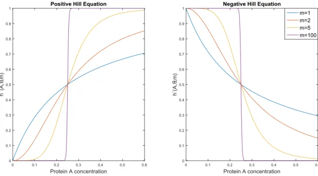
and approaches unity [92] and h−(A, θ, m) describes the opposite case. The parameter θ is the expression threshold of the protein A necessary to produce a significant increase of mRNA and the parameter m is called Hill coefficient. It controls the steepness of the Hill functions (the higher is m, the more step-like is the Hill function): if m = 1 the function is then called the Michaelis-Menten equation. Figure 4.2 shows the steepness of Hill functions at different values of m.

Protein A concentration 0 0.1 0.2 0.3 0.4 0.5 0.6 h +(A, θ,m) 0 0.1 0.2 0.3 0.4 0.5 0.6 0.7 0.8 0.9

1 Positive Hill Equation

Protein A concentration 0 0.1 0.2 0.3 0.4 0.5 0.6 h -(A, θ,m) 0 0.1 0.2 0.3 0.4 0.5 0.6 0.7 0.8 0.9

1 Negative Hill Equation

m=1 m=2 m=5 m=100

Figure 4.2: Hill function. Positive (resp. negative) Hill function on the left (resp. right) for different Hill coefficients: m=1 (Michaelis-Menten case), 2, 5, 100. The

(46)

Figure 4.3: Classical model of gene regulation. The regulation of the gene G by the protein A.

Translation can be modeled as a linear function of mRNA concentration with a degra-dation term as well [20]:

˙

P = κ2M − γPP. (4.9)

Therefore the classical model of gene regulation is:    ˙ M = κ0+ κ1h+(A, θ, m) − γMM, ˙ P = κ2M − γP P. (4.10)

The gene G is transcribed in the M mRNA and the latter is translated in the protein P . The transcription of the gene is regulated by the protein A, see Figure 4.3.

4.1.2 Quasi-steady-state assumption of mRNA concentration

It is possible to further simplify the system using the quasi-steady-state-assumption (QSSA) [103]. QSSA is an well-known approximation method in biochemical kinetics an and other fields, simplifying the ODE systems with two relevant time scales (fast and slow scale).

Most of the time mRNA dynamics in GRNs is much faster than protein dynamics, i.e. the mRNA concentration reaches its equilibrium faster than that of the protein (typical mRNA half-lives are 2-6 minutes, while those of proteins are on the order of hours [8]). So, in System (4.10), the mRNA M is degrading faster than the protein P (γM ≫ γP):

because mRNA concentrations reaches its equilibrium point - the point where ˙M = 0 - on a time scale much quicker than the concentration of the protein, we can apply the QSSA in System (4.10).

We now consider the case with an activator protein [20]. We do a time variable change (τ = γPt) and we obtain the scaled system:

dM dτ = κ0 γP + κ1 γP Am θm A + Am −γM γP M, (4.11)