Analysis and design of an in-pipe system for water leak detection

(1)

Analysis and Design of an In-Pipe System for

Water Leak Detection

MASSACHUSEIFS INSTITUTE

OF TECH LOY

NO

03 v

2 by

Dimitris M. Chatzigeorgiou

Submitted to the Department of Mechanical Engineering

in partial fulfillment of the requirements for the degree of

Master of Science in Mechanical Engineering

at the

MASSACHUSETTS INSTITUTE OF TECHNOLOGY

September 2010

@

Massachusetts Institute of Technology 2010. All rights reserved.

Author ...

Department of Mechanical Engineering

August 27, 2010

Certified by ...

[...

A

'

Kamal Youcef-Toumi

Professor of Mechanical Engineering

Thesis Supervisor

VA

Accepted by ... r .-...

David E. Hardt

Chairman, Department Committee on Graduate Students

(2)

(3)

Analysis and Design of an In-Pipe System for Water Leak

Detection

by

Dimitris M. Chatzigeorgiou

Submitted to the Department of Mechanical Engineering on August 27, 2010, in partial fulfillment of the

requirements for the degree of

Master of Science in Mechanical Engineering

Abstract

Leaks are a major factor for unaccounted water losses in almost every water distribu-tion network. Pipeline leak may result, for example, from bad workmanship or from any destructive cause, due to sudden changes of pressure, corrosion, cracks, defects in pipes or lack of maintenance. The problem of leak becomes even more serious when it is concerned with the vital supply of fresh water to the community. In addition to waste of resources, contaminants may infiltrate into the water supply. The pos-sibility of environmental health disasters due to delay in detection of water pipeline leaks have spurred research into the development of methods for pipeline leak and contamination detection.

This thesis is on the analysis and design of a floating mobile sensor for leak

detec-tion in water distribudetec-tion pipes. This work covers the study of two modules, namely

a "floating body" along with its "sensing module".

The Mobility Module or the floating body was carefully studied and designed using advanced CFD techniques to make the body as non-invasive to the flow as possible and to avoid signal corruption. In addition, experiments were carried out to investigate the effectiveness of using in-pipe measurements for leak detection in plastic pipes. Specifically, acoustic signals due to simulated leaks were measured and studied for designing a detection system to be deployed inside water networks of 100mm pipe size.

Thesis Supervisor: Kamal Youcef-Toumi Title: Professor of Mechanical Engineering

(4)

(5)

Acknowledgments

At this point I would like to thank my advisor, Professor Kamal Youcef-Toumi, for his valuable advice and patience throughout the duration of this work. His energy and enthousiasm in research had motivated me and made my research life smooth and exciting. I would also like to thank him for giving me the chance to participate in three "Clean Water and Clean Energy" workshops, one of them held in Dhahran, Saudi Arabia and was a wonderful experience.

Secondly, I wish to thank all my lab buddies, Dan Burns, Mauricio Gutierrez, Kwang Yong Lim, Vijay Shilpiekandula, and Sang-il Lee for making me feel com-fortable and part of the group from day one. Additionally I would like to thank Prof. Sanjay Sarma, Dr. Atia Khalifa, Dr. Ajay Deshpande, Sumeet Kumar and Dr. Stephen Ho for their help and great advice throughout this work.

Next, I would like to thank my good friends here in Boston, who stood by me in good and bad during those two years at MIT and gave meaning to my after-lab-life every single day from day one to day seven-hundred-twenty-nine. Buddies, I wouldn't have managed to finish this work without you.

My deepest gratitude goes to my family for their unflagging love and support

throughout my life; this thesis is simply impossible without them. Miss you all back there in Greece.

I would also like to thank the Onassis Public Benefit Foundation for their support

and for believing in me from the very beginning of this work.

I would finally like to thank the King Fahd University of Petroleum and Minerals

(KFUPM) in Dhahran, Saudi Arabia, for funding the research reported in this thesis through the Center for Clean Water and Clean Energy at MIT and KFUPM.

This thesis is dedicated with all my heart to my newborn niece. She is now six months old and is adorable. I had the chance to meet her last month in Greece. My whole family is excited about her. I am looking forward to seeing her again...

(6)

(7)

List of Figures

1-1 Schematic of the mobile floating sensor concept. The pipeline is buried

underground and the "yellow" mobile sensor is floating, while at the same time communicating with the "outer world" and sensing for leaks. 21 1-2 The four different subsystems of the floating mobile sensor. . . . . 22 2-1 Leak detection in water pipelines using the Sewerin Aquaphone A100.

[Picture from www.sewerin.com] . . . . 26

2-2 Typical Leak Noise Correlators. Sensor A, Sensor B and Correlator

device. [Courtesy of Dantec Measurement Technology] . . . . 27

2-3 Tracer Gas technique sketch. . . . . 28

2-4 The RADIODETECTION RD1000 Portable Ground Penetrating Radar System . . . . . 29 2-5 Some state-of-the-art leak inspection robots. . . . . 33 2-6 Top Left: Un-tethered Autonomous Kurt I, Top Right: CISBOT,

Bot-tom : GRISLEE . . . . 33 2-7 A typical leak detection survey with the Smartball. . . . . 35 2-8 Sketch of the Sahara leak detection system. . . . . 35 3-1 The hydrophone 8103 from B&K. Picture taken from http://www. bksv.com 40

3-2 The receiving frequency response of the hydrophone sensor 8103 from

B&K. Graph taken from http://www.bksv.com . . . . 41

3-3 The WB-1372 DeltaTron Power Supply from B&K. Picture taken from

(12)

3-4 The Charge to Delta Tron converter type 2647 from B&K. Picture taken

from http://www.bksv.com . . . . 41

3-5 The Dynamic Pressure Sensor 106B52 from PCB Piezotronics. Picture

taken from http://www.pcb.com . . . . 42

3-6 A sketch describing all the subsystems within the dynamic pressure

sen-sor 106B52 from PCB Piezotronics. Picture taken from http://www.pcb.com 43

3-7 The 482A21 Sensor Signal Conditioner from PCB Piezotronics.

Pic-ture taken from http://www.pcb.com . . . . 43

3-8 The SR560 amplifier from Stanford Research Systems. . . . . 44

3-9 The National Instruments 9234 24bit analog input module. Picture

taken from http://www.ni.com . . . . 45

3-10 The National Instruments 9113 chassis. Picture taken from http://www.ni.com 45 3-11 The National Instruments 9022 real-time controller. Picture taken

from http://www.ni.com . . . . 45

3-12 The user interface in LabVIEW for DAQ . . . . 47 4-1 Test loop in the lab consisting mostly of 100mm ID pipe sections . . 50 4-2 The solid model of the test loop . . . . 50

4-3 The solid model of the sensor-holder used to hold and move the hy-drophone along the pipe. The sensor holder part is sketched in brown co lor. . . . . 5 1

4-4 The actual sensor-holder while moving the hydrophone along the pipe. Magnets on both sides are used to move the sensor. . . . . 52

4-5 The DPS is mounted flush on the pipe body. The hydrophone is mounted on the sensor holder and is moving with the use of mag-nets from the outside. The 1/8" valve simulating a leak is also shown

in the picture. . . . . 52

4-6 The 1/8" valve simulating a leak. . . . . 53

(13)

5-1 Signals captured by [a] DPS and [b] hydrophone for the case of a

10lit/min leak. Pressure in the pipe is 45psi. The time signal as

well as the frequency spectrum of each case are shown. . . . . 58

5-2 Signals captured by [a] DPS and [b] hydrophone for the case of a

14lit/min leak. Pressure in the pipe is 38psi. The time signal as

well as the frequency spectrum of each case are shown. . . . . 60 5-3 Signals captured by [a] DPS and [b] hydrophone for the case of a

6lit/min leak. Pressure in the pipe is 50psi. The time signal as well

as the frequency spectrum of each case are shown. . . . . 61

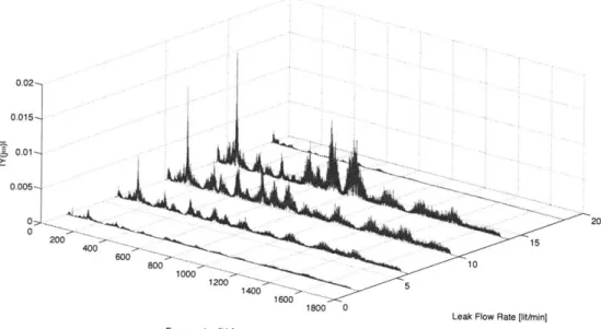
5-4 The frequency spectra for the signals captured by the DPS for different leak flow rates. The sensor is placed at the leak position. . . . . 63 5-5 The frequency spectra for the signals captured by the hydrophone for

different leak flow rates. The sensor is placed at the leak position. . . 63 5-6 Leak signals for 1mm up to 6mm leak sizes. The frequency spectrum

for each case is presented. Leak is open to air. . . . . 65 5-7 The test section for the "sand" experiments. A tank filled with sand

was used. Leak jet was hitting the sand at the bottom. . . . . 68 5-8 The frequency spectra of the leak signals captured in air/sand/water.

Green/Air, Orange/Sand and Red/Water. Power of the signal in sand and water is more than the same power for the signal in air. Moreover the frequency spectra is "wider" for those two cases in comparison to the "air experim ents". . . . . 68 5-9 Effect of having pipe flow on frequency spectrum - sensor used:

hy-drophone... ... 72 5-10 Effect of pipe flow rate on leak signal for constant leak flow rate of

8it/min - sensor used: DPS . . . . 73 5-11 Effect of pipe flow rate on captured signal; pipe flow 8lit/min - sensor

used: D P S . . . . 73 5-12 Calculated power of leak signal with and without pipe flow - sensor

(14)

5-13 Frequency spectra for signals captured for 4mm leak; Pipe is

sur-rounded by water and the hydrophone was placed at different positions upstream and downstream of the leak location . . . . 75 6-1 The design of the mobility module. [Left] Front View. [Right] Side

v iew . . . . . 79 6-2 A zoom in the mobility module's solid model. Explanation on different

parts is sketched. ... ... ... 79

6-3 The 3D solid model of the mobility module. Model is shown inside a

100m m pipe section. . . . . 80

6-4 The 3D printed prototype of the leg. Material is ABS plastic. .... 82 6-5 The 3D printed prototype of the upper part of the external hull.

Ma-terial is A BS plastic. . . . . 83 6-6 The 3D printed prototype of the lower part of the external hull.

Ma-terial is ABS plastic. . . . . 84

6-7 The 3D printed parts of the mobility module. Material is ABS plastic. 85 6-8 The assembled mobility module. . . . . 85 6-9 The prototype

#

3. . . . . 86 6-10 The prototype

#

4. The module inside the pipe is shown in the left

figure. The details of the leg are presented in the right figure. .... 87 6-11 The prototype

#

6. . . . . 87 7-1 A 2D sketch of a cylindrical mobility module inside a bended pipe.. 90 7-2 Maximum allowed thickness Hmax of the mobility module for a given

length L... ... ... 91

7-3 The design of the mobility module. [Left] Front view. [Right] Side

view . . . . . 92

7-4 Body is floating within the pipe with speed Vm, while water speed is V. 93

7-5 Body can be considered to be stationary in this case and water is flowing at a lower speed, namely Vre = V - Vm. Notice that in this frame of reference the pipe wall is also moving with Vm. . . . . 93

(15)

7-6 The response of the system's velocity for the following values: V" =

lm/s, m = 1kg, CD 0.4, A = .0165m2, p = 998kg/n 3 and the

initial condition is: Vm(0) = 0m/s. The response is presented for

different values of Feg, varying from 0.5 to 3N. Notice that by applying larger friction forces through the legs, the module travels with smaller speeds and can even "anchor" itself (Vm = 0). . . . . 95 7-7 The mesh used for the CFD analysis on the mobility module. The mesh

on the inlet, outlet sections as well as the floating body is presented. . 97

7-8 M esh of the fluidic section. . . . . 97 7-9 CFD results for velocity vectors around the floating body. Simulation

was done under Vre = 2 m/s (direction from right to left (see Fig. 7-5) and P = 200kPa. No flow separation on the trailing edge. . . . . 100

7-10 CFD results for static pressure distribution around the floating body.

Simulation was done under Vre = 2 m/s (direction from right to left (see Fig. 7-5) and P = 200kPa. Placing the sensor nose at the trailing

edge seems to be the optimal solution. . . . . 101

7-11 CFD results for static pressure distribution around the floating body.

Simulation was done under Vre = 0.01 m/s (direction from right to left

(see Fig. 7-5) and P = 200kPa. Almost no pressure variation around

the body. ... ... 101

8-1 The mobility module prototype inside a 100mm pipe section. The

module is stable, due to the support provided by the legs . . . . 104

8-2 The mobility module floating through section A of the experimental

setup. The six photos ([a]-[f]) show the motion of the mobility module from left to right. . . . . 106 8-3 The mobility module floating through section B of the experimental

setup. The six photos ([a]-[f]) show the motion of the mobility module from left to right. . . . . 107

(16)

8-4 The mobility module floating through the right branch of section C of the experimental setup. The six photos ([a]-[f]) show the motion of the mobility module from right to left. . . . 108 8-5 The mobility module floating through the left branch of section C of

the experimental setup. The three photos ([f]-[h]) show the motion of the mobility module from right to left. . . . . 109 A-1 The front panel of the LabVIEW vi on the host PC. User can select

"AC/DC/IEPE" in the "Input Configuration" box. One can also spec-ify the sampling rate along with the number of scans per survey. A

"Stop" button is available in order to be able to stop the procedure at any time. Various indicators including a "Waveform Graph" are also available for the user. . . . . 116 A-2 The front panel of the LabVIEW vi on the FPGA. User can select

"AC/DC/IEPE" in the "Input Configuration" box. One can also spec-ify the sampling rate. A "Start" and "Stop" button are available in

this vi. Indicators including "Buffer Underflow" and "Buffer Overflow" are also shown in this interface. . . . . 116 A-3 The first part of the block diagram of the LabVIEW vi on the host PC.

Notice that this part is connected to the second part shown in Fig. A-4.117 A-4 The second part of the block diagram of the LabVIEW vi on the host

PC. Notice that this part is connected to the first part shown in Fig. A -3 . . . . . 118 A-5 The third part of the block diagram of the LabVIEW vi on the host

PC. Notice that this part is not connected to neither of the first or

second parts shown in Fig. A-3 and Fig. A-4. . . . . 119 A-6 The first part of the block diagram of the LabVIEW vi on the FPGA.

Notice that this part is connected to the second part shown in Fig. A-7.120

A-7 The second part of the block diagram of the LabVIEW vi on the FPGA.

(17)

List of Tables

5.1 Summary of measured leak flow rate and line pressure for different leak sizes. . . . . 64

5.2 Signal Power calculation for each leak case. The ratio of each power relative to the no-leak case is also presented. Standard deviation is also presented to show repeatability of signal power. . . . . 66 5.3 Signal Power calculation for each leak case. The ratio of each power

relative to the no-leak case is also presented. . . . . 69

5.4 Power calculations for various positions upstream, downstream and at leak position . . . . 75 7.1 M esh characteristics . . . . 98

(18)

(19)

Chapter 1 Introduction

1.1 Problem Definition

"What is a leak and where does it come from?" The unintentional release of fluid

from a pipeline can be defined as "leak". Pipeline leaks may result, for example, from bad workmanship or from any destructive cause, due to sudden changes of

pressure, cracks, defects in pipes or lack of maintenance. Water transmission and distribution networks may deteriorate with time due to corrosion, soil movement, poor construction standards and sometimes also due to excessive traffic loads or even induced vibration.

1.2 Motivation

In most cases, the deleterious effects associated with the occurrence of leaks may present serious problems and, therefore, leaks must be quickly detected, located and repaired. The problem of leak even becomes more serious when it is concerned with the vital supply of fresh water to the community. In addition to waste of resources, contaminants may infiltrate into the water supply. The possibility of environmental health disasters due to delay in detection of water pipeline leaks have spurred research into the development of methods for pipeline leak and contamination detection.

(20)

es-pecially in countries where water is scarce. This issue has stimulated our interest towards the design and development of a mobile floating sensor for accurate leak detection in water distribution networks.

Leaks in water pipes create acoustic emissions, which can be sensed to identify and localize leaks. Leak noise correlators and listening devices have been reported in the literature as successful approaches to leak detection but they have practical limitations in terms of cost, sensitivity, reliability and scalability. A possible efficient solution is the development of an in-pipe traveling leak detection system. In-pipe sensing is more accurate and efficient, since the sensing element can get very close to the sound source. Currently in-pipe approaches have been limited to large leaks and larger diameter pipes.

The development of such a system requires clear understanding of acoustic signals generated from leaks and the study of the variation of the signal with different pipe loading conditions, leak sizes and surrounding media. It also requires a "careful" design of the system that will be traveling along the water pipes while at the same time carrying the corresponding sensors for leak detection.

1.3 Thesis Objectives

The objective of this thesis is the analysis and design of an appropriate floating mobile sensor for the in-pipe sensing of leaks within a water distribution network. In this thesis, this includes the study of two different things, namely the "Sensing Module" as well as the "Mobility Module". A brief description of each one of them is presented in the following paragraphs. A schematic of the mobile floating sensor is presented in Fig. 1-1.

The autonomous in-pipe leak detection system consists of four different modules (Fig. 1-2); each of which has its own significance and role. A brief summary of each module is presented here. Note that this thesis focuses only on the first two modules.

* Sensing Module: The sensing module is the module in the system that is

(21)

Figure 1-1: Schematic of the mobile floating sensor concept. The pipeline is buried underground and the "yellow" mobile sensor is floating, while at the same time com-municating with the "outer world" and sensing for leaks.

of the sensing module requires the development of an appropriate technique for in-pipe leak detection. In addition the sensing module's design part includes first of all understanding of the physical phenomenon of a leaking pipe and in addition to that the experimentation and selection of the appropriate sensors and instrumentation for accurate leak detection.

The sensing module may also carry other sensors as well, e.g. sensors for local-ization. This thesis is focused on the leak detection sensing element only.

" Mobility Module: The mobility module is the module in the system on which

the sensor and all other instrumentation will be mounted. Moreover, the design of the "floating body" needs to be carefully studied because the deployment of a mobile sensor in a pipe network can be considered as an invasive detection technique. Thus, the body itself needs to be as less "invasive" to the flow field as possible to avoid signal corruption.

" Communications Module: This module is responsible for the communication

between the in-pipe floating system and an above ground receiver. Experimen-tal investigation of the signal propagation through different media (sand, clay, water, etc.) is needed to improve the design of this module. Discussion of this

(22)

Figure 1-2: The four different subsystems of the floating mobile sensor. module is outside the scope.of this thesis.

o Data Processing Module: This module is responsible for post-processing the data stemming from the sensing module as well as the communications module. The miniaturized memory storage technology is currently available but the power requirements to process large amount of data are still challenging for the present design. Discussion of this module is outside the scope of this thesis.

1.4 Structure of the Thesis

Chapter 2 discusses the background and literature review of concurrent leak detection techniques. The sensing module is discussed in chapter 3, while the experimental setup that was designed and built is presented in chapter 4. Finally the experimental results and corresponding analyses for leak detection are discussed in chapter 5.

Next, chapter 6 presents the design of the mobility module and chapter 7 the corresponding analysis. Finally chapter 8 discusses the experiments conducted on the mobility module using the experimental setup described in chapter 4. Our conclusions and recommendations for future works are stated in chapter 9.

(23)

Chapter 2 Background

2.1 Introduction

This chapter discusses the state-of-the-art leak detection methods and robotic devices. Those different techniques are listed and evaluated as per efficiency and limitations. The most critical functional requirements of a "floating mobile sensor" are also listed in this chapter.

2.2 Water Losses

Potable water is a critical resource to human society. Failure and inefficiencies in transporting drinking water to its final destination wastes resource and energy. With limited access to fresh water reserves and increasing demand of potable water, water shortage is becoming a critical challenge. So, addressing water losses during distri-bution presents significant opportunity for conservation.

Leaks are the major factor for unaccounted water losses in almost every water distribution network; old or modern. Vickers [1] reports water losses in USA munici-palities to range from 15 to 25 percent. The Canadian Water Research Institute [2] reports that on average, 20 percent of treated water is wasted due to losses during dis-tribution and other unaccounted means. A study on leakage assessment in Riyadh, Saudi Arabia shows the average leak percentage of the ten studied areas to be 30

(24)

percent [3]. Losses through leaks represent a significant portion of the water supply, hence identification and elimination of leaks is imperative to efficient water resource management.

Unaccounted water losses include metering errors, accounting errors and some-times theft; however, typically the greatest contributor to lost water is caused by leaks in the distribution pipes [4],[5]. Failure at joint connections is the usual cause for leaks in pipes. Corrosion, ground movement, loading and vibration from road traffic all contribute to pipe deterioration over time and eventual failure [5]. Old or poorly constructed pipelines, material defects, inadequate corrosion protection, poorly maintained valves and mechanical damage are some other factors contributing to leaks [6].

2.3 Leak Detection Techniques

2.3.1 Overview

In this section some of the most significant concurrent methods for leak detection in pipelines will be discussed.

Water Audits - Metering

Mays [4] and Hunaidi [5] report various techniques for leak detection. Water losses can be estimated from water audits. The difference between the amounts of water produced by the water utility and the total amount of water recorded by water usage meters indicates the amount of unaccounted water. District metering offers a slightly higher level of insight into water losses than bulk accounting by isolating sections of the distribution network (into districts), measuring the amount of water entering the district and comparing the amount of water recorded by meters within the district. While the amount of unaccounted water gives a good indication of the severity of water leakage in a distribution network, metering gives no information about the locations of these losses.

(25)

Listening Devices

Acoustic equipment and more specifically "listening devices" have been widely used

by water authorities worldwide for locating leaks in water distribution networks [5].

These include various systems, among them: " Listening Rods

* Aquaphones .

" Geophones (Ground Microphones)

All listening devices are based on the same "sensing" technique, since all of them

are using sensitive materials such as piezoelectric elements to sense leak-induced sounds and/or vibrations. Those sensing elements are usually accompanied by some signal amplifiers and filters to make the leak signal stand out. The operation of those listening devices is straight-forward, but the efficiency depends on the user's experience [7].

To operate a listening device an experienced user is required. The user carries the equipment above ground, tries to follow the pipe map and at the same time is focused on pinpointing a "high-amplitude" acoustic signal with his headset or his monitor (Fig. 2-1).

Leak Noise Correlators

The state of the art in leak detection techniques lies on the "Leak Noise Correlators". Those devices are more efficient, get more accurate results and depend less on user experience than the listening devices [8].

Leak Noise Correlators are portable microprocessor-based devices that use the cross-correlation method to pinpoint leaks automatically. In most cases either vibra-tion sensors (e.g. accelerometers) or acoustic sensors (e.g. hydrophones) are used at two distinct pipe locations (usually in openings within a water distribution network, such as fire hydrants) that of course need to bracket the location of the suspected leak. If the leak is located somewhere between the two measurement points but not

(26)

Figure 2-1: Leak detection in water pipelines using the Sewerin Aquaphone A100. [Picture from www.sewerin.com]

in the middle, then there is a time lag between the measured leak signals by the two distinct sensors. This time lag is pinpointed by the cross-correlation function of the leak signals. The location of the leak can be easily calculated using a simple algebraic relationship using the time lag, the distance between the sensors and the propagation velocity of the wave signal in the pipe

[91.

This method is destined to fail if there are more than one leaks present between the correlators, which is a very common case in real networks. Another problem associated with this method is that there are cases when there is no access to the pipe close to the leak. In these cases a deployment of a mobile sensor is necessary. Moreover, they can be unreliable for quiet leaks in cast and ductile iron pipes and for most leaks in plastic and large-diameter pipes. Correlators are also expensive and remain beyond the means of many water utilities and leak detection service companies. A typical leak noise correlator is shown in Fig. 2-2.

(27)

Figure 2-2: Typical Leak Noise Correlators. Sensor A, Sensor B and Correlator device. [Courtesy of Dantec Measurement Technology]

Pressure Transients

Pressure transients have been used to formulate inverse transient algorithms for leak detection and localization of both single and multiple leaks. Inverse transient for-mulation involves collecting pressure data during the occurrence of transient events followed by minimization of the difference between observed and estimated param-eters. The estimated parameters are calculated through hydraulic transient solvers

[10],

[11]. The method has shown success in detecting leaks in laboratory conditions

under high leak flow rates. Karney studied the applicability and effectiveness of in-verse transient analysis to the detection of leaks in real water distribution systems [12]. This method constitutes a low-cost and easy-to-implement alternative; however its feasibility has yet to be fully established in actual field conditions. In addition, there are risks of introducing controlled transients into the distribution system. The method relies on the availability of an accurate transient model of the network and system parameters that are often impractical or expensive to obtain.

(28)

Tracer Gas Technique

Several non-acoustic methods like infrared thermography; tracer gas technique and ground-penetrating radar (GPR) have as well been explored as potential leak detec-tion methods. Tracer Gas Technique involves the injecdetec-tion of a non-toxic, insoluble in water gas, into an isolated pipe section. The gas is then pressurized and able to exit the pipe through a leak opening and then, being lighter than air, permeates to the surface through the soil and pavement. The leak is located by scanning the ground surface directly above the pipe with a highly sensitive gas detector (Fig. 2-3).

Figure 2-3: Tracer Gas technique sketch.

Thermography

The principle behind the use of thermography for leak detection in water-filled pipes is that water leaking from an underground buried pipe is changing the thermal field of the adjacent soil. The resulting temperature gradients can be picked up by the corresponding equipment, e.g. infrared cameras. The method requires scanning of the pipe network above ground and the procedure is almost the same as in the GPR or the Tracer Gas Technique. An experienced user is required to walk, following the map of the network and searching for leaks in the pipe network.

(29)

Ground-Penetrating Radar (GPR)

This technique uses a radar that can detect voids in the soil created by leaking water as it circulates near the pipe, or segments of the pipe which appear to be buried deeper than they are because of the increase of the dielectric constant of adjacent soil saturated by leaking water.

GPR waves are partially reflected back to the ground surface when they encounter an anomaly in dielectric properties, for example, a void or pipe [13]. An image of the size and shape of the object is formed by radar time-traces obtained by scanning the ground surface. The time lag between transmitted and reflected radar waves determines the depth of the reflecting object. A typical GPR device is presented in Fig. 2-4.

Figure 2-4: The RADIODETECTION RD1000 Portable Ground Penetrating Radar System.

2.3.2 Summary and Evaluation

In this section the most efficient leak detection techniques will be summarized and evaluated as per advantages, limitations, cost and accuracy. Pros and cons of each

(30)

method will be presented in table form.

Listening Devices : Locating the loudest sound of leak by sound transducers placed

on the ground surface above the pipe.

+

Most commonly used - Depends on the operator skills

+

Acceptable accuracy - Not effective for small leaks

+

Simple to carry and move - Affected by background noise - Depends on pipe size, material

- Depends on water table level, system pressure - Loose soil muffles sound

- Exact pipe location must be known

- More suitable for hard surfaces

- Depth less than 2 m

Acoustic with Correlation : A correlation algorithm uses two vibration

trans-ducers' signals installed on the pipe at two locations bounding the leak with pipeline information.

+

Good accuracy - Leak should be between two listening points

+

Acceptable price - Fails in case of multiple leaks

+

Minimal operator training - Accuracy relies on input of pipe features - Not suitable for plastic pipes

- Good sensor contact is essential

- Accuracy depends on the distance of the leak to measuring points

- Sometimes there is no access to the pipe close to the leak

- External noise interferes with the signals

(31)

detected at ground surface.

+ Effective method in case

of emergency that requires isolating the pipe with no flow

- Very expensive

- Time consuming

- Exact pipe location must be known

- Limited to depth less than 2 m

Thermography : Locating the temperature differences in soil caused by leaking

water using infrared radiation.

+

Non-contact, nondestructive - Very expensive

+

Able to inspect large areas - Significant operator experience

from above ground with - Detection depends on the soil

100% coverage characteristics, leak size, and burial depth

+Locates

subsurface leaks as - Application limited by ambient conditions well as voids and erosion

surrounding pipelines

Ground Penetrating Radar : Uses electromagnetic radiation of the radio

spec-trum, and detects the reflected signals from subsurface structures. It detects voids created by the leaking water or anomalies in the depth of the pipe due to soil saturation with leaking water.

+

Variety of media - Significant operator experience

± Detects objects, voids, cracks - Expensive (hardware & software)

+

Penetration up to 15m - High energy consumption

- Depth of penetration depends on

soil type

All methods discussed so far are searching for leaks above the ground with all the

(32)

inspection is much more accurate, less sensitive to random events and external noise and also more deterministic, due to the fact that it is less subjective to the user's experience. Moreover, pipe inspection from the inside brings the "sensing module" closer to the source and consequently the system itself is capable of pinpointing very small leaks. In general such systems face difficult challenges associated with commu-nication, powering and are in general expensive to build.

2.4 Inspection Robots

In the area of in-pipe inspection systems, there are many examples of prior-art robotic systems for use in underground piping. Most of them are however focused on water-and sewer-lines, water-and meant for inspection, repair water-and rehabilitation. Some examples are shown in Fig. 2-5. As such, they are mostly tethered; utilizing cameras specialized tooling and usually are designed to operate in empty-pipe-conditions.

Beaver

Pe~ii

Figure 2-5: Some state-of-the-art leak inspection robots.

Three of the more notable exceptions are the autonomous Kurt I system from

GMD used for sewer monitoring, the tethered gas main cast-iron pipe joint-sealing

robot CISBOT and the GRISLEE robot, Fig. 2-6. The latter is a coiled-tubing tether deployed inspection, marking and in-situ spot-repair system.

(33)

Figure 2-6: Top Left: Un-tethered Autonomous Kurt I, Top Right: CISB0 T, Bottom:

GRISLEE

(34)

There are also robots that have been developed for in-pipe inspection such as corrosion, cracks or normal wear and damage. State of the art robots are usually four-wheeled, camera carrying and umbilically controlled. Most of them are however focused on oil or sewer-mains. One of the most successful steps in building such a robot was developed by Schempf at CMU [14] with his untethered Explorer robot. The system is a long-range, leak-inspection robot, working in real-gas-pipeline conditions and is being controlled by an operator in real-time through wireless RF technology. The operator is constantly looking to a monitor and is searching for leaks visually via a camera.

Kwon built a reconfigurable pipeline inspection robot with a length of 75mm and a modular exterior diameter changing from 75mm up to 105mm [15]. Controlling the speed of each one of the three caterpillar wheels independently provides a steering capability to the system.

Most of the state-of-the-art leak detection robots are able to travel along horizon-tal pipelines and only a small fraction of them can cope with complicated pipeline configurations, e.g. T-junctions, bended pipes etc. Even if some of them manage to cope with that they usually require a complete shut-down of the network and deployment of the system in an empty pipe such as the MRINSPECT [16].

The Smartball is a mobile device that can identify and locate small leaks in water pipelines larger than 254 mm (10") in diameter constructed of any pipe material

[17], as shown in Fig. 2-7. The free-swimming device consists of a porous foam

ball that envelops a water-tight, aluminum sphere containing the sensitive acoustic instrumentation. This device is capable of inspecting very long pipes but cannot handle complicated pipeline configurations.

Bond presents a tethered system that pinpoints the location and estimates the magnitude of the leak in large diameter water transmission mains of different con-struction types [18]. Carried by the flow of water, the system can travel through the pipe and in case of a leak, the leak position is marked on the surface by an operator, who is following the device (Fig. 2-8). The system is tethered and thus all range limitations apply in this case.

(35)

Figure 2-7: A typical leak detection survey with the Smartball.

Figure 2-8: Sketch of the Sahara leak detection system.

Leak Detection and Condition Alssessment

(36)

2.5 System Functional Requirements

As presented in the previous sections many methods have been developed over the last few decades to detect leaks in water pipes. Leak detection using in-pipe sensing came to picture recently by different systems. Nevertheless, all of the state-of-the-art systems have limitations.

Our goal is to design a system that tackles the main problems and overcomes some of the limitations. The functional requirements of such a system may be listed as follows:

" Autonomy: The system should be completely autonomous (untethered). The system will be deployed in one point and will be retrieved from another point in the pipe network.

" Leak Sensing Sensitivity: The system is aimed at detecting "small" leaks in plastic (PVC) pipes (depending on the sensing element). Plastic pipes are the most difficult for leak detection [19], since sound and vibrations are greatly damped over small distances away from the leak. Thus, detecting leaks in plastic pipes requires deploying a mobile sensor that should be very close to the leak.

" Working Conditions: System will be deployed under the real pipe flow

condi-tions, more specifically:

- Line Pressure: 1 to 5 bars

- Flow Speed: 0.5 to 2 m/s (in 100mm ID pipes which corresponds to a volumetric flow rate of up to 15.7 lit/sec).

" Communication: The system needs to be able to communicate with stations above ground and pinpoint potential leaks in the water network.

" Localization: The system needs to be able to localize itself within the water

distribution network. This is essential for the accurate leak position estimation and the retrieval of the sensor from the network as well.

(37)

2.6 Chapter Summary

In this chapter various leak detection methods, systems and robotic devices have been listed and evaluated. Water audits, listening devices, leak noise correlators, pressure transients, tracer gas technique, infrared thermography and GPR are all promising techniques with advantages as well as limitations. The idea of an in-pipe moving sensor "'swimming" along a pipeline and detecting leaks from the inside seems to be challenging but at the same time promising and more accurate, since the sensor will get very close to the source as it passes by the leak. Such a system has some functional requirements, that are also presented in this chapter.

(38)

(39)

Chapter 3 Sensing Module

-

Instrumentation

3.1 Introduction

This chapter will discuss the sensing module characteristics, i.e. the sensors' charac-teristics and the instrumentation used to acquire the signal in terms of both hardware and software. Specific details and specifications of the instrumentation that we used for experimentation will be given.

3.2 Sensor Overview and Characteristics

For the accurate leak detection two different sensors have been used. The first one is a hydrophone, presented in section 3.2.1, while the second one is a Dynamic Pressure Sensor (DPS). The latter one and its characteristics are discussed in section 3.2.2. Both of them are able to measure dynamic pressure fluctuations as we will see in the next sections.

3.2.1 Hydrophone

The hydrophone that we used in our experiments is a B & K system with model number is 8103. This specific model is of a small size, high-sensitivity transducer for making absolute sound measurements over the frequency range 0.1Hz to 180kHz

(40)

DoubL- hi elde -Lown Cabe 70-0CuN-Suppot Contro (0,374") 2232

Figure 3-1: The hydrophone 8103 from B&K. Picture taken from

http://www. bksv. corn

with a receiving sensitivity of -211 dB with reference to 1V/ptPa, which corresponds to 25.9 puV/Pa or approximately. 0.1786 V/psi. It has a high sensitivity relative to its size and good all-round characteristics, which make it generally applicable to laboratory, industrial and educational use. Type 8103's high frequency response is especially valuable when making acoustic investigations of marine animals and in the measurement of the pressure-distribution patterns in ultrasonic-cleaning baths. It is also useful for cavitation measurements. Fig. 3-1 shows the sensor and its main dimensions. Fig. 3-2 shows the frequency response of the hydrophone as measured by the company after calibration. The flat frequency response over a large frequency range even at very low frequencies was the main reason why this product was selected for our experiments. The weight of the sensor plus the cable is 170 grams.

To power up this sensor we used the WB-1372 Delta Tron. Power Supply from B&K

(Fig.

3-3). A Charge to Delta Tront converter was also necessary, so we selected the type 2647 from BBiK (Fig. 3-4).

(41)

=Njj-- JfType

8103-2 5 10 20 50 100 200 500 1 kHz 5 10 20 50 100kHz

Figure

B&K.

3-2: The receiving frequency response of the hydrophone sensor 8103 from

Graph taken from http://www.bksv.com

Figure 3-3: The WB-1372 DeltaTron Power Supply from BLK. Picture taken from http://www.bksv.com

Figure 3-4: The Charge to DeltaTron converter type 2647 from B&K. Picture taken from http://www.bksv.com

-200 -210 -220

(42)

3.2.2 Dynamic Pressure Sensor (DPS)

The DPS that we used is model 106B52 from PCB Piezotronics. This is a very sensitive model with a sensitivity of 5V/psi and a resolution of 2 x 10-5. This sensor has also a very flat frequency response starting from approximately 2.5Hz. The resonant frequency takes place at very high frequencies of the order of > 40kHz. The weight of this sensor is 35 grams. Fig. 3-5 shows a picture of the sensor while Fig.

3-6 presents a small sketch of all different subsystems within the sensor. To power

up this sensor we used the 482A21 Sensor Signal Conditioner from PCB Piezotronics (Fig. 3-7).

Figure 3-5: The Dynamic Pressure Sensor 106B52 from PCB Piezotronics. Picture taken from http://www.pcb-com

3.3 Instrumentation Characteristics

Except for the sensors and their accessories other instrumentation was used to acquire data and drive the signal to the host PC and store it before postprocessing. Those will be discussed in this section.

3.3.1 Amplifier

In all of our experiments with the hydrophone we used a low-noise voltage preampli-fier. More specifically the model that we used was the SR560 from Stanford Research

(43)

AC CELERAT1ON COMIPENSATION CRYSTAL MASS PRELOAD SLEEVE CRYSTAL END PIECE CONNEC TOR \ TEGRATED HOUSING DIAPHRAGM

Figure 3-6: A sketch describing all the subsystems within the dynamic pressure sensor

106B52 from PCB Piezotronics. Picture taken from http://www.pcb.com

/ 7,

7~

Figure 3-7: The 482A21 Sensor Signal Conditioner from PCB Piezotronics. Picture taken from http://www.pcb.com

(44)

The amplifier provides a variable gain from 1 to 50,000, either AC or DC coupled inputs and outputs as well as line or battery operation. It is also equipped with two configurable signal filters that the user can adjust according to will and apply low-, high- or even band-pass filter to the input signal. Filter cutoff frequencies can be set in a 1 - 3 - 10 sequence from 0.03 Hz to 1 MHz. A picture of the amplifier is shown

in Fig. 3-8.

Figure 3-8: The SR560 amplifier from Stanford Research Systems.

3.3.2 Data AQuisition (DAQ) Hardware

The data acquisition system that was used consists of four different parts that are described in this section. For DAQ the signal is driven to a National Instruments 9234 4-channel, 51.2kHz maximum sampling rate, 24bit analog input module (Fig.3-9). This one sits on a National Instruments cRIO-9113 Reconfigurable Chassis

(Fig.3-10). The system is driven by a National Instruments cRIO-9022 real-time controller

with 256MB DDR2 RAM and a 533MHz processor (Fig.3-11). The controller is supplied with ethernet ports and by using one of them we connect it to the Host PC, where we record and post-process the signals.

(45)

Figure 3-9: The National Instruments 9234 24bit analog input module. Picture taken from http://www.ni.com

Figure 3-10: The National Instruments 9113

http://www.ni.com

chassis.

Figure 3-11: The National Instruments 9022 real-time controller. http://www.ni.com

Picture taken from

(46)

3.3.3 Connection Overview

Hydrophone Connection Overview

A charge to voltage Delta Tron converter is connected in series with the hydrophone

and the sensor is powered by the Delta Tron WB 1372 module. The output of the later module is then connected to a power amplifier and signal conditioner from Stanford

Research Systems. The output of the amplifier is directed to the NI 9234 module on

a cR10-9113 reconfigurable chassis. The sampling rate can be selected manually by the user and can go up to 51.2KHz. Signal is finally driven from the DAQ FPGA to the host PC for postprocessing.

DPS Connection Overview

The DPS has a built-in amplifier and produces 5V for 1 psi pressure fluctuation, so there is no need to connect it to the amplifier. It is directly connected to a 1-channel, line- powered, ICP sensor signal conditioner model 482A21 which provides constant current excitation to the sensor. The output of this power supply is directed to the

NI 9234 module on a cRIO-9113 reconfigurable chassis. The sampling rate can be

selected manually by the user and can go up to 51.2KHz. Signal is finally driven from the DAQ FPGA to the host PC for postprocessing.

3.3.4 Data AQuisition (DAQ) Software

The DAQ software that we used consists of a couple of LabVIEW virtual instruments (vi's). The user is able to select the sampling rate

f,

for the DAQ. The various options for the sampling rate are

f,

= 51, 200/n Hz, where n = 1, 2 ....30, 31. This means that the sampling rate range starts at 1652Hz and goes up to 51200Hz. The user is also able to see a real-time graph of the time-series signal captured. The interface that the user is able to see on the host PC under LabVIEW is presented in Fig. 3-12. For more information on the DAQ software please refer to Appendix A.

(47)

Figure 3-12: The user interface in LabVIEW for DAQ.

3.4 Chapter Summary

This section discusses the sensors, their accessories and the required hardware that were used to acquire the signals from the sensors and store them for postprocessing.

A small description and detailed specifications of each module are described, as well

(48)

(49)

Chapter 4 Sensing Module

-

Experimentation

4.1 Introduction

This chapter will discuss the experimental setup used to detect leaks in water pipes. An overview of the setup sections, as well as a description of the objectives of this experimental work will be given.

4.2 Experimental Setup Overview

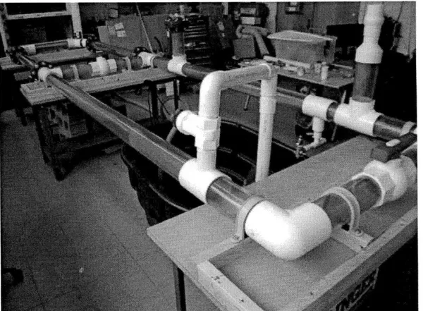
The setup used for experimentation is shown in Fig. 4-1. It consists of 100mm ID plastic pipes (1.5m long), with the municipality water supply fed at one end, while the other end is fitted by a flow control valve. Fig. 4-2 shows the solid model of the test loop with some brief explanation on some features.

This setup allows pipe flow rates from 0 to 23 lit/min, which are considered very small, compared to actual network flows but they satisfy the current experimental objectives. A pressure gage is installed on the pipe for measuring the line pressure. The leak flow rate is measured using an Omega flow meter (Model FDP301) which can be used to measure flow rates as low as 0.3 lit/min.

A hydrophone is used to listen to leak noise and a dynamic pressure sensor (DPS) is

used to pick up the water pressure disturbance due to the leak. Both the hydrophone and the pressure transducer can move relative to the leak location; upstream or

(50)

Figure 4-1: Test loop in the lab consisting mostly of 100mm ID pipe sections

Test section

(1.5m long) Section for sensor_insertion

z Air release valve

P/

Tank

Inlet section

(51)

downstream. The hydrophone was always centered at the centerline of the pipe being supported by a plastic 3D-printed part, see Fig. 4-3. The later one was moved along the pipe using magnets (Fig.4-4). The DPS is mounted flush on pipe wall using special adapter. The different installation of the hydrophone and the DPS is presented in Fig. 4-5.

Figure 4-3: The solid model of the sensor-holder used to hold and move the hy-drophone along the pipe. The sensor holder part is sketched in brown color.

4.3 Simulating Leaks

The simulated leaks are of two different types. Firstly, we simulated a leak by using a

1/8" (3.175mm) PVC valve and the valve opening is controlled based on the required

leak flow rate (Fig. 4-6). A second type is simulated by drilling corresponding holes on the test section (Fig. 4-7). Each drill bit resulted in a different leak size with a different flow rate. Thus, leaks in this case are simulated by circular holes on the pipe body.

(52)

Figure 4-4: The actual sensor-holder while moving the hydrophone along the pipe. Magnets on both sides are used to move the sensor.

Figure 4-5: The DPS is mounted flush on the pipe body. The hydrophone is mounted on the sensor holder and is moving with the use of magnets from the outside. The

(53)

Figure 4-6: The 1/8" valve simulating a leak.

4.4 Experimentation Objectives

The objective of this experimentation is to characterize acoustic emissions stemming from a leak, simulated as a circular hole or a small valve, on a plastic water pipeline using a hydrophone or DPS. Experiments were done with 100mm ID PVC pipes, which is commonly used material and size in modern water distribution networks. Our goal was to come up with a "metric" or a way for leak detection.

The following parameters/conditions are to be studied during this experimentation for the sensing module:

* Leak size

" "Ambient" pipe flow

" Surrounding medium

(54)

Figure 4-7: The circular hole simulating a leak.

(55)

4.5 Chapter Summary

In this section the experimental loop that was built for experimentation was discussed and its features were described. The different ways leaks were simulated are also presented. Finally, the objectives of the experimental work for the sensing module are listed.

(56)

(57)

Chapter 5 Sensing Module

-

Experimental

Results

5.1 Introduction

This chapter will present the experimental results on leak detection using the hard-ware and softhard-ware presented in chapter 3 as well as the experimental setup discussed in chapter 4.

5.2 Hydrophone vs DPS

The first objective is to test the two sensors and understand their characteristics. To do so, we test the sensors under similar experimental conditions and study the captured signals. Signals for the same flow rates under the same conditions will be compared. To satisfy this experimental matrix, both the DPS and the hydrophone are used for signal capturing with a controlled leak to provide the basic knowledge on the previously mentioned objectives. Leak is simulated using a 1/8" PVC valve and the valve opening is controlled based on the required leak flow rate. Experiments were carried out with no pipe flow (pipeline end is closed). The pipe flow can be varied between 0 to 23 lit/min. Leak is always open to air for this set of experiments.

(58)

0.5 lbI. -' leak 101pm dps 45psi 0.1 0.2 0.3 0.4 0.5 0.6 0.7 0.8 0.9 Time [sec]

Single-Sided Amplitude Spectrum of y(t)

200 400 600 800 1000

Frequency

[-1200 1400 1600 1800 2000

[a] Signal captured by DPS leak 101pm hydrophone 45psi

5 - ..

-.-.-0 0.1 0.2 0.3 0.4 0.5 0.6 0.7 0.8 0.9 1

Time [sec]

X 10-3 Single-Sided Amplitude Spectrum of y(t)

2 1 5 5 . . .. . . . .. .. . . . . .. . . 0 200 400 600 800 1000 1200 1400 1600 1800 Frequency [Hz] 2000

[b] Signal captured by hydrophone

Figure 5-1: Signals captured by [a] DPS and [b] hydrophone for the case of a 10lit/min leak. Pressure in the pipe is 45psi. The time signal as well as the frequency spectrum of each case are shown.

-0.5 0.02 0.015 0.01 0.005 0 0.0 E <-0. 0 -0. -. . .. . .. .. .. ... . . .. .. .. . .. . . . ... ~ .~~ . .. .. . .-.. . ..-.. .-. . . .. . -. ..-. .-. .- ..-0

Analysis and design of an in-pipe system for water leak detection

Analysis and Design of an In-Pipe System for

Water Leak Detection

NO

03 v

2

by

Dimitris M. Chatzigeorgiou

Submitted to the Department of Mechanical Engineering

in partial fulfillment of the requirements for the degree of

Master of Science in Mechanical Engineering

at the

MASSACHUSETTS INSTITUTE OF TECHNOLOGY

September 2010

@

Massachusetts Institute of Technology 2010. All rights reserved.

Author ...

Department of Mechanical Engineering

August 27, 2010

Certified by ...

[...

A

'

Kamal Youcef-Toumi

Professor of Mechanical Engineering

Thesis Supervisor

David E. Hardt

Chairman, Department Committee on Graduate Students

Analysis and Design of an In-Pipe System for Water Leak

Detection

by

Dimitris M. Chatzigeorgiou

Abstract

Acknowledgments

Contents

List of Figures

#

#

#

List of Tables

Chapter 1

Introduction

1.1

Problem Definition

1.2

Motivation

1.3

Thesis Objectives

1.4

Structure of the Thesis

Chapter 2

Background

2.1

Introduction

2.2

Water Losses

2.3

Leak Detection Techniques

2.3.1

Overview

[91.

[10],

2.3.2

Summary and Evaluation

+

+

+

+

+

+

+

+

+Locates

+

+

2.4

Inspection Robots

Beaver

Pe~ii

Leak Detection and Condition Alssessment