Data processing in nanoscale profilometry

Data Processing in Nanoscale Profilometry

by

Cheng-Jung Chiu

Submitted to the Department of Mechanical Engineering

in partial fulfillment of the requirements for the degree of

Master of Science in Mechanical Engineering

at the

MASSACHUSETTS INSTITUTE OF TECHNOLOGY

() Massachusetts Institute

May 1995

of Technology 1995.

All rights reserved.

A utho r

... ...

Departmen of Mechanical Engineering

d b y . A -i Y - ,.

-Dr. Kamal Youcef-Toumi

Associate Professor

Thesis Supervisor

Accepted by.

A ccepted by .

...

....

...

Dr. Ain A. Sonin

Chairman, Departmental Committee on Graduate Students

MASSACHUSETTS INSTITUTE OFTECHNOLOGY

FEB 1 6 201

3arker Bt

Data Processing in Nanoscale Profilometry

by

Cheng-Jung Chiu

Submitted to the Department of Mechanical Engineering

on May 12, 1995, in partial fulfillment of the

requirements for the degree of

Master of Science in Mechanical Engineering

Abstract

New developments on the nanoscale are taking place rapidly in many fields. Instru-mentation used to measure and understand the geometry and property of the small scale structure is therefore essential. One of the most promising devices to head the measurement science into the nanoscale is the scanning probe microscope. A proto-type of a nanoscale profilometer based on the scanning probe microscope has been built in the Laboratory for Manufacturing and Productivity at MIT. A sample is placed on a precision flip stage and different sides of the sample are scanned under the SPM to acquire its separate surface topography. To reconstruct the original three dimensional profile, many techniques like digital filtering, edge identification, and im-age matching are investigated and implemented in the computer programs to post process the data, and with greater emphasis placed on the nanoscale application. The important programming issues are addressed, too. Finally, this system's error sources

are discussed and analyzed.

Thesis Supervisor: Dr. Kamal Youcef-Toumi Title: Associate Professor

Acknowledgments

At the outset, my gratitute goes to my thesis advisor, Professor Kamal Youcef-Toumi. for his guidance, patience, and kindness. Thank him for giving me the chance to work on this project. help me learned so many things here. Also thank Dr. Eric Liu's guidance and advices in this project. The discussions with him provides me many. many ideas.

I would like to thank my collaborator Tarzen Kwok, for his tireless input and assistance. He not only supported and helped me in many parts of this project through the end of the thesis. his working altitude also lets me realize how to do research.

I also want to thank T.J. for his generous advices. He is always willing to listen to my problems and give me the appropriate suggestions, both in the research and ill my personal life. I'm glad I can work with him in the same laboratory.

I also thank all the colleagues and friends I made here. Mingchih. Ilin. .Jane. Mingyi. Cynthia. and many, mans' more. They mades my life at MIT has been more productive and enjoyable.

Finall. I have to thank my family and say sorry that I couldn't accompany them in the past two years. Thank my sister Ya-Ting and my brother Cheng-Wei for the love and cheer they shared with me. Most importantly. I would like to thank ily parents. who give me their unconditional support. endless love and care. They made

me know the joy of life. Their loving always encourages me while I'm down. If I could

Contents

1 Introduction

1.1 Motivation . 1.2 Thesis Contents.

2 System Configuration and Operation 2.1 introduction.

2.2 System Description ...

2.2.1 AFM machine .

2.2.2 Sample Positioning System . 2.3 Operation Procedure. 2.4 Summary ... 12

... . 12

....

12

... .

14

... .

14

... .

15

....

17

3 Data Acquisition and Processing 3.1 Introduction. 3.2 Filtering (Noise Removal) ... 3.2.1 Lowpass Filtering ... 3.2.2 Median Filtering. 3.2.3 Adaptive Wiener Filtering .... 3.3 Data Reconstruction (Deconvolution) . . 3.4 Edge Identification. 3.4.1 First-Derivative-Based Method 3.4.2 Second-Derivative-Based Method 3.5 Image Matching ... 19 . . . 19 . . . 21 . . . 23 . . . .. 23 . . . 24 . . . 2 5 . . . 29 . . . 30 . . . 31 . . . 33 10 10 11

3.6 Images Combination. 3.6.1 Simplified Method 3.6.2 Corrected Method 3.7 Summary ... 4 Software Implementation 4.1 Instroduction ... 4.2 Data Structure. 4.3 User Interface.

4.4 Software Operation Procedure 4.5 Summary ...

5 Errors Analysis 5.1 Introduction.

5.2 AFM-Related Errors.

5.2.1 Piezo Actuator . . . .

5.2.2 Cantilever and Tip 5.3 Positioning Stages . 5.4 Thermal Drift. 5.5 Summary ...

6 Conclusion

A Coordinate Transformation

B Optimal Sample Tilt Angle for Scanning C Software Functions

C.1 Programming Environment ... C.2 Software Operation ... D List of Program Codes

D.1 afmproj.ide. 35 37 39 41 43 43 44 45 46 48 49 49 50 50 56 58 65 66 67 69 71 73 73 75 82 82

...

...

...

...

...

...

...

...

...

...

...

...

...

...

...

...

D.1.1 afmproj5.def. D.1.2 afmproj5.h. D.1.3 afmproj5.c D.1.4 afmproj5.rc D.1.5 seladlg.rc D.2 matrxlib.ide .... D.2.1 matrxlib.def D.2.2 matrxlib.h. D.2.3 matrxlib.c D.3 afmlib.ide ... D.3.1 afmlib.def D.3.2 afmlib.h D.3.3 afmlib.c

D.4 filesel.ide...

...

...

...

...

...

...

...

...

...

...

...

...

...

List of Figures

2-1 Overall System Configuration ... ... 13

2-2 Schematic of a Generalized Atomic Force Microscope ... 13

2-3 Flip Stage ... 15

2-4 Typical Scanning Trace ... 16

2-5 Different Profiling Results Due to the Tip's Orientation [16] ... 18

3-1 Image Shifting ... 20

3-2 Filtered Image and the Identified Edge: (a) Raw Image (b) FIR Low-pass Filtering (c) Median Filtering (d) Wiener Filtering ... 22

3-3 Examples of Influence of Tip Shape to Apparent Surface Profile [4] 25 3-4 Envelop Image Analysis[5] ... 26

3-5 Envelop Image Analysis with Noise[5] ... 28

3-6 Envelop Image Analysis for a Tip with Upward Convex Shape ... . 29

3-7 Deconvolution with Noise (a) Envelop Image Analysis (b) Localize En-velop Image Analysis to the Tip Area ... 30

3-8 Edge Detection[10] ... 31

3-9 Simulation of Sample Edge Detection (a) with a Simple Tip (b) with a More Realistic Tip ... 32

3-10 Image Matching . . . ... 33

3-11 Matching of Two Sides Sample Images ... 35

3-12 System Coordinations Definition . . . 36

3-13 Coordinate System for Corrected Method ... 39

4-1 Matlab Program Interface ... ... 44

4-2 Software User Interface ... 47

5-1 (a) Piezoelectric Tube[13] (b) Tripod Scanner [2] ... 50

5-2 Nonlinearity of Piezoelectric (a) Intrinsic Nonlinearity (b) Hysteresis (c) Creep (d) The Effect of Creep to a Step Sample [13] ... 52

5-3 Effect of Tube Tilting on the Lateral Displacement of the Tip or Sample[4] 54 5-4 AFM Images of a Linear 9.9 gm-pitch grating: (a) Without x-y, and z Independent Position Sensors (b) With Position Sensors ... 55

5-5 AFM Images of an Optical Flat Sample (a) Without z Position Sensor (b) With z Position Sensor (c) Fitting a Second-Order Surface to (b) 56 A-1 Coordinate Transformation ... 70

B-1 Sample and Tip ... 72

C-1 user interface ... 76

C-2 File Selection Window . . . ... 77

C-3 Setting Window ... 79

C-4 Parameters for Edge Identification . . . 79

List of Tables

5.1 Error Gains for Position 1 ... 62

Chapter 1

Introduction

1.1 Motivation

New developments on nanoscale are taking place in many fields. Therefore, the in-strumentation to understand and measure the geometry and properties of the small scale structure to nanometric resolutions are essential. One of the most promising devices to lead the measurement science into the nanoscale precision is the Scanning Probe Microscope. Scanning Probe Microscope (SPM) was first invented in the early 1980's. The extremely high resolution it provides (up to a few anstroms) made it be used widely in a variety of disciplines, including surface science, microstructure study. biomedical analysis, ... etc. Its high resolution ability along with scanning range up to 100 pm also makes it suitable as a "micro coordinate measuring machine".

An atomic-force-microscope-based nano-precision profilometer has been designed and implemented at the Laboratory for Manufacturing and Productivity at Mas-sachusetts Institute of Technology 1. The device is primarily used to measure the profile of the sample tip area. The sample is kinematically clamped to the reference surface of the sample jig (flip stage) under the AFM scanner. After one side measure-ment is finished, the sample is flipped over by rotating the high precision flip stage to measure the other side. Using the edge identification and image matching techniques.

the separate parts of the sample surface topography could be reconnected and the original three dimensional sample profile can be reconstructed.

All the styli-type profiliometers are suffered from the measurement distortion caused by the convolution between the tip shape and the measured surface, especially if the surface has steep slope or sharp edge. This situation occurs in the scanning of this sample's tip area. Based on David Keller's deconvolutoin method [5], the convolution problem can be reduced.

1.2 Thesis Contents

The thesis is organized as follows. Chapter 2 describes the basic configuration of the profilometer, it includes X-Y stages, flip stage and AFM machine. A brief operation procedure to measure a sample is given here, too.

The post-processing issues are addressed in Chapter 3. To recover the original sample profile from the noisy, distorted, and separated two side data, technique such as discrete filtering, deconvolution, edge identification, image matching and coordi-nate transformation are adopted.

Chapter 4 described some essential issues about software implementation. The data processing software are currently developed under MS-Windows environment to provide the graphical user interface. A brief operation procedure for this program is introduced here, too.

Chapter 5 is focused on the system's performance, or errors analysis. The system's error sources , including the AFMI\, positioning and flip stages, are reviewed. Some errors can be avoided or reduced by software or hardware methods, others are difficult to eliminate at least in this machine. They are all evaluated in this chapter.

Chapter 2

System Configuration and

Operation

2.1 introduction

The whole system used to measure the sample profile could be decomposed into three parts: the commercial AFM machine (from the Park Scientific Instruments, XL). the custom sample positioning system, this includes a sample flip stage and X-' positioning stages, and post-processing software. This chapter will briefly describe the first two parts, or the hardware configuration. Also, the measuring procedure will be covered here. Topics about the post processing issues (software part), like filtering, reconstruction, ...etc are addressed in the next chapter.

2.2 System Description

The outline of the customized AFM machine is shown in Figure 2-1 . It consists a commercial AFM machine, X-Y' stages and a flip stage. The coordinate system is defined as follows : the X axis is parallel to the reference mounting surface (i.e. the granite table) and pointing into the sample, the Y axis is on the centerline of rotation

Figure 2-1: Overall System Configuration

(i.e. along the sample edge), and the Z axis is normal to the granite surface.

2.2.1 AFM machine

Basically, in the contact mode atomic force microscope, a cantilever beam mounted microstylus is moved relative to the sample surface using piezoactuators, (see Fig-ure 2-2); and the deflection of the cantilever is taken to be a measFig-urement of the surface topography. The AFM used throughout this thesis work is a commercial ma-chine from the Park Scientific Instruments. It can provide a scanning range up to

1.00x100l m in lateral and 8 im in vertical (the Z direction), also it has a

closed-loop/independent sensor monitoring of piezoelectric scanner motion to eliminate the errors from piezoelectric scanner's intrinsic nonlinear behavior. This makes it a suit-able choice as a miniature CMM. Also, it comes up with a high magnitude CCD camera which makes the automated sample positioning possible.

2.2.2

Sample Positioning System

The sample positioning system is composed of X-Y stages and a flip stage.

The X-Y stages provides the required resolution to locate the sample at the desired measuring position in X and Y' direction 2 while providing the required mechanical

stability to get the nanometer level measurement. The stage also provides the long range movement of the sample for ease of loading.

A close-up look of the flip stage is shown in Figure 2-3. [7] The flip stage has two main functions : one is to hold the sample and provide a reference plane for the sample, the other is to provide the required high precision and high repeatable rotary movement for measuring the two sides of a sample. The sample is clamped against a reference surface plane by a clip and aligned to the axis of rotation (the line connecting the centers of two locator balls) by two precision stops. The axis of rotation is defined by the X-Y-Z and roll/yaw stops on the bases and two locator balls

2_{the coarse positioning in Z direction is accomplished by a stepping motor which moves the}

Z

V~~~

-- X

Figure 2-3: Flip Stage

on the sample holder. To position at the tilt angle, the sample holder is rotated to the near vicinity of the angle stop by a geared stepping motor; once there (i.e. position sensed by a limit switch) power to the motor is shut off and the holder is magnetically clamped against the angle stop. The X-l'-Z stop, constructed out of three balls, the yaw/roll angle stops, consisting of two rods that form a 'V' two point constraint, and the axis locator balls on the sample holder form a kinematic mechanism to provide the required high repeatability. To unclamp, the motor is reenergized and made to turn in the opposite direction.

2.3 Operation Procedure

The essential profiling procedure consists of the following operations: 1. Set up the AFM and load the sample;

Figure 2-4: Typical Scanning Trace

2. Visually align the sample ultimate edge with the probe tip ( in the X direction) and lower the AFM probe onto the sample surface, then use the AFM piezoscan-ner for lateral alignment with the ultimate tip; a single trace line should show a step-like feature, it means that the profile contains data both before and after the scanning tip falls off the sample edge. A typical sample profiling seen on the digital oscilloscope on the computer screen is shown in Figure 2-4.

3. Appropriately setting the AFM measurement parameters; two important things not usually seen in the surface topography measurement are pointed out. One is the scanning direction. Scanning direction should be from the sample body to the sample edge, this can reduce the piezoscanner's creeping error, also in this way, the transient error from the surface changes (like a step response) happened after the scanning tip has fallen off the sample's ultimate tip, and those data are not important for profile reconstruction later 3. Another thing to notice

is to turn off "autoslope". In the usual surface topography measurement, the data measured will be fitted a first order plane to remove the surface tilting component from the stages and the scanner (autoslope). But this is not the

case here. The data from two sides of the sample should be measured with respect to the same reference coordinate system, so the "autoslope" should be turned off.

4. Flip the sample to the other side and repeat steps 2 and 3 5. Post process the measurement data4

One thing worthy to mention is, the scanning direction is set in the X direction while the sample's edge is parallel to the Y direction. These arrangements have the following benefits :

1. Because the cantilever is mounted parallel to the Y direction and the scanning tip is on the center line of the cantilever, it is easier to align the sample by looking at the center line of the cantilever if the sample edge is parallel to the 1Y direction instead of the X direction.

2. Because the scanning tip is tilted at a certain angle in the Y-Z plane, it will cause a different level of convolution problems due to the asymmetry of the scanning tip if the different scanning direction is taken . (for example., if we scan a step sample from -Y to +Y and then from +Y to -Y', because of the

asymmetry of the tip's sidewall to the Z direction, the slope gradient at the step area will be different as shown in Figure 2-5). To reduce this problem, the

scanning direction should be set in the X direction.

2.4

Summary

In this chapter, the hardware configuration of the profilometer was described. Some design features and consideration in this instrument were included. The operation procedure to measure a sample was also addressed. Again, the detailed design process

for this instrument can be found in Kwok[7].

4_{See chapter 4} 5

1500 x [nm] (c) - cantilever

tip

Figure 2-5: Different Profiling Results Due to the Tip's Orientation [16]

(b) z [nm] 400 200 0 hole rel 500 1000 0

_o4f

Chapter 3

Data Acquisition and Processing

3.1 Introduction

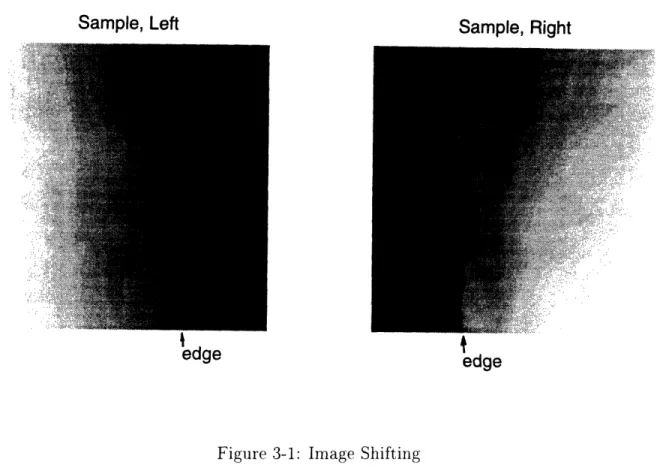
The data gathered from the profilometer represents only a sample's two separate surface topography. The critical issue is to transform these surface topography into the original sample profile. A typical profiling trace from the AFM is shown in Figure 2-5. This curve shows how a scanning tip moves along a sample surface. It contains information not only the sample profile but also the interaction between the scanning tip and the sample. It is also mixed with some irrelevant data. (i.e.: the data after the tip has fallen off the sample's ultimate edge.) Besides, the data is also contaminated by noise and disturbance. Unless the falling point can be identified first and the sample profile can be extracted from the noise-contaminated, extra-information-mixed data. the true three dimensional profile is hard to be established. One thing to note is, the rotation of the flip stage will not only flip the sample over, it will also introduce some errors like the shifting along the sample edge. As shown in Figure 3-1, by comparing the edge features of the two images, we can see that the images are not matched very well, there is shifting along the edge direction and the left image is lower than the right image. This error needs to be effectively compensated by use of image matching technique before putting the two sides images together.

Sample, Right

edge _edge

Figure 3-1: Image Shifting

implemented and tested here. First. the data is passed through a discrete filter to effectively reduce the noise. To eliminate the error from the finite size of the scanning tip (convolution problem between the tip and the sample edge), the "envelope image analysis" method developed b David Keller[5] is adopted to deconvolute the probe shape from the scanning profile. Then an edge identification technique is used to find the sample edge. At the assumption of the sample edges identified from the two sides images are the same, by use of coordinate transformation, the original three dimensional sample profile can be established.

Here is the list of the essential procedures 1. discrete filtering of the data.

2. reconstructing the data by use of the "envelop image analysis" method. 3. identifying the sample edges of the two images.

4. image matching to correct the data shifting.

5. coordinate transformation to establish the whole profile. The detailed procedures are described in the following sections.

3.2 Filtering (Noise Removal)

Basically, the scanning data from the AFM can be looked as a digital image. Noise can corrupt the data or image analysis in many ways, especially in edge detection of a image, a discrete approximation of first or second derivatives of the image data are commonly needed, and the noise can seriously distort the edge identified since differentiation will amplify those high frequency noise. Examples of additive noise degradation here could be electronic circuit noise, environment noise from acoustic or thermal effects, and even amplitude quantization noise. Basically, those noise can be taken as random and vuncorrelated.

An image degraded by additive random noise can be modeled by

g(nl,,

n

)

=

f(nl,

)

+ v(nl,

(3.1)

where f(nl, n2) is the original, ideal image, v(nl, n2) represents the signal

indepen-dent, additive random noise and g(nl, n2) represents the corrupted image. n and n2

are the indices of the pixel.

If every v(nl, n₂) is uncorrelated with zero-mean, then by scanning the sample's

same area many times and averaging those images up, the noise could be reduced. Unfortunately, due to the time constraint and other problems like thermal drifting and the wearing of the scanning tip, this is infeasible.

To effectively reduce the noise, A few smoothing techniques commonly used in image processing have been tested and compared.

FIR Lowpass Filtering (a) Median Filtering (b) Wiener Filtering (c) _(d)

Figure 3-2: Filtered Image and the Identified Edge: (a) Raw Image (b) FIR Lowpass Filtering (c) Median Filtering (d) lWiener Filtering

3.2.1

Lowpass Filtering

Since the energy of a typical image noise contains higher frequency component com-pared to the true image, by reducing the high frequency components while preserving the low-frequency components, lowpass filtering reduces a large amount of noise at the expense of reducing a small amount of signal. As shown in Figure 3-2 (a) and (b), compared to the unfiltered image, lowpass filtering does reduce the additive noise, and smooth the "wiggle" of the identified sample edge, 2 but at the same time it blurs (distorts) the image. Blurring is a primary limitation of the lowpass filtering, espe-cially at the border of the image or the area with significant changes. Experiments

found that, compared to the other filtering methods (median and Adaptive Wiener filtering, see below), lowpass filtering causes more distortions at the identified edge points.

3.2.2 Median Filtering

Median filtering is a nonlinear process useful in reducing impulsive or salt-and-pepper noise. It is also useful in preserving edge in an image while reducing random noise. In a median filter, a window slides along the image, and the median intensity value of the pixels within the window becomes the output intensity of the pixel being processed. For example, suppose the pixel values within a window are 5, 6, 55, 10. and 15, and the pixel being processed has a value 55. The output of the median filter at the current pixel location is 10, which is the median of the five values. Like lowpass filtering, median filtering smoothes the image, but it can preserve discontinuities in a step function and smooth a few pixel whose values differ significantly from their surroundings without affecting the other pixels.[10]

To better preserve 2D step discontinuities, the separable median filtering method are adopted, that is, the 2-D signal is filtered in one direction with 1-D median filter first, then filtered in the perpendicular direction. The result of separable median filtering depends on the order in which the 1-D horizontal and vertical median filters

2

are applied. In the sample scanning data, since the horizontal direction is taken as the raster scanning direction, the noise of the adjacent pixels in the vertical direction can be looked as uncorrelated, so it is preferable to filter in the vertical direction to remove the most significant noise first, then filter in the horizontal direction. Figure 3-2 (c) shows the filtered image and the edge detected.

3.2.3 Adaptive Wiener Filtering

In Equation (3.1), if signal f(nl, n2) and the noise v(nl, n2) are samples of

zero-mean stationary random processes that are linearly independent of each other and their power spectra Pf(w1, w2) and Pv(wl, w2) are known, the minimum mean square

errors estimate of f(nl, n2) is obtained by filtering g(nl, n2) with a Wiener filter whose

frequency response H(wl, w2) is given by

H(wlP wj2,)= (W1,W2) (3.2)

H(w w2 Pf(wl, w2) + P,(w, w2)3

If f(nl, n2) has a mean of mf and v(nl, n2) has a mean of m, then mf and m, are

first subtracted from the degraded image g(nl, n2). The resulting signal g(nl, n2) -(mf + m,) is next filtered by the Wiener filter. The signal mean mn is then added to

the filtered signal.

Basically, the Wiener filter preserves the high SNR frequency components while attenuating the low SNR frequency components. Since the noise is generally wideband compared to the signal, the Wiener filter's lowpass characteristics can effectively

reduce the noise. But, just like the usual lowpass filtering, Wiener filter blurs the image significantly. One reason is that a fixed filter is used throughout the entire image. In a typical image, image characteristics differ considerably from one region to another. Degradation may also vary from one region to another. It is reasonable, then, to adapt the processing to the changing characteristics of the image and degradation.

One adaptive Wiener filter developed by Lee [8] has the form below

p(nl

mf(nln

)

+

+

g(nl,n

) - mfr(ni

n2))

(3.3)

(a) Probe .-Scan Line .... . X-·--~ r !' ~% i ·· · ·' ·: .:: ::., - .I '. .','" · . : '., ',....- .. -. _{:··~~~~~~I:} .~: : · .,-..:!7. ..:-.' : <::.(i?~~~~~~~~4.;:···:. ~'....,: ::~ i":"":"' '.:. ....

i-

Figure 3-3: Examples of Influence of Tip Shape to Apparent Surface Profile [4]

where p(nl, n2) is the processed image, mf and of are the local mean and standard

deviation of f(nl, n2) and are updated at each pixel. the additive noise v(n1,n2) is

assumed to be zero mean and white with variance of 2. Again, to further preserve

the edge, a cascade of 1-D adaptive Wiener filtering can be applied. Figure 3-2(d) shows the filtered image and the edge detected. First, the 1-D filter is oriented in the same direction as the edge, the edge can be avoided and the image can be filtered along it. Then another 1-D filter that crosses the edge is applied.

Comparing the curves of the detected sample edges in Figure 3-2 (a)-(d), we found that filtering does effectively remove the noise and is helpful for further analysis. To this particular application, the adaptive Wiener filtering shows better performance over the other filtering methods tested.

3.3 Data Reconstruction (Deconvolution)

One difficulty in probe metrology arises when a surface has regions with steep slopes. How faithfully a probe microscope shows the surface topography depends strongly on the size and shape of the probe. Ideally, the scanning tip should have a impulse-like shape, or a tip which is much sharper and its sidewalls are much steeper than any feature in the sample, then the resulting image will closely follows the actual sample surface. But in practice. due to manufacturing issues, also taking into account the

Figure 3-4: Envelop Image Analysis[5]

stiffness of the scanning tip, the tip is seldom ideal. Then some features may be

completelv inaccessible while others will be distorted. Figure 3-3 shows how a tip

shape might effect the output profile. The distortion comes from the relative motion of the tip and the sample while scanning, which strongly depends on the shape of the tip and usually is a nonlinear process. 3 Unless the size and shape of the probe are accurately known, the distortion cannot be corrected. One wav to acquire the actual tip shape is to scan the tip under another microscope, for example, SE.M. Another feasible way is to scan a particular, well-defined sample with shape known beforehand [5]. Once the tip shape is acquired, there are a few methods available to reduce this

problem. (e.g., Keller et al. [5][6], Lee et al.[9].) One effective method is the "envelope

image analysis" method proposed by Keller[5] to reconstruct the distorted image. The envelope image analysis method computes the reconstructed sample surface as the envelop of a large set of probe tip surface functions. If the sample is considered to be beneath the tip, so the tip surface is assumed to be downward-pointing and to have a well defined minimum, which will be called the end point of the tip. By

3

Although the process of extracting the true profile from the distorted data are usually referred to "deconvolution", actually, care must be taken. Since "convolution" is a linear process, but here, it is highly non-linear in the common case. Deconvolution techniques like Fourier Transformation cannot be used here.

placing the tip surface on each point of the image surface, as shown in Figure 3-4, the reconstructed sample surface is the envelop formed by all of such tip surface. The advantages of this method over the other methods is that no particular tip shape needed (e.g., Lee et al. [9]) and less noise-sensitive compared to some other methods. ( e.g., Niedermann et al. [11], Reiss [15].)

As we can see from Figure 3-4, there are certain regions ( "unreconstructable" regions) that can not be reconstructed no matter how accurate the data may be. The region between the contact points is never touched by the probe, so the image contains no informations about it. And in this method, they are filled with a segment of the tip surface. This segment needs to be identified so the sample profile can be extracted there (see section 3.4).

To implement the above method into a computer program, a mathematical de-scription is needed. Consider an image surface z(x,y), defined in a region R of the xy plane. Let the surface of the probe tip be given by a function t(x,y), usually, it is convenient to define the minimum point of the tip shape as the ori-gin. Let (x,y) and (x',y') be two points in the xy plane, and define a function

w(x, y; x', y') = z(x', y') + t(x - x', y - y'). Here w(x, y; x', y') is effectively a tip

func-tion with its axis located at (x', y') and with its end point raised to a height z(x', y'). Then the reconstructed surface, r(x, y), is the minimum of all functions w(x, y; x', y') over all (x', y') in R. so that

r(x, y) = min z(x', y') + t(x - x', y - y'), all (x', y') in R (3.4)

for each point (x, y) in R. For this expression to be defined, w(x, y; x', y') must have a minimum, i.e., both z(x, y) and t(x, y) must have lower bounds.[5]

One common problem of all the deconvolution methods is, either the tip or the sample's true profile must be known beforehand. Here, the tip shape must be ac-curately measured or estimated if high accuracy is needed. But, even in the same manufacturing batch, the tips are different from each other, also it takes time to acquire the accurate tip profile. Other factors like the tip's tilt angle will also effect

(a)

(b)

Figure 3-5: Envelop Image Analysis with Noise[5]

the convolution result, and this error will cause a sine error or the so called Abb6 principle.

Another problem comes from the image noise. Although the envelop image anal-vsis method can effectively remove a sharp, upward fluctuations (Figure 3-5 (a)), but for a downward fluctuation, it will produce a significant distortion in the reconstructed surface (see Figure 3-5 (b)).

To eliminate these problems, the envelop image analysis method should be applied only to the small ultimate tip area. Basically, the envelop image analysis method reconstructs the data from a scanning tip's downward convex shape part. For a tip with upward convex shape or just a straight line, the envelop image analysis method can not provide more information. From Figure 3-6, we can see that, unlike a tip with downward convex shape, for a ideal tip with only upward convex shape, the scanning profile and the reconstructed profile are exactly the same. Most SPRM tips are parabolic-like only quite near the ultimate tip end. Further up, the tip surface usually goes over to an approximately downward convex conical shape or even a straight line. So, only the ultimate tip area will actually effect the reconstructed

profile.

The advantage of restricting this method only to the ultimate tip area is that

only the estimation or measurement of the ultimate tip shape is needed, and the deconvolution errors due to inappropriate tip information can be minimized. Also the deconvolution errors from the image noise can be reduced in some cases, too.

scanning profile 1 0.5 0

-0.5

Figure 3-6: Envelop Image Analysis for a Tip with Upward Convex Shape Figure 3-7 shows, the restricted envelop image analysis method causes less distortion to the downward fluctuation of noise compared to the original method.

3.4 Edge Identification

Once the image is reconstructed from the noised and distorted data, the next step is to find the intermediate point between the sample profile and the unreconstructable region filled by the tip shape, or the "edge".

In an image system, an edge is a boundary or contour at which a significant change occurs in some physical aspect of an image, such as the changes in image intensity. This is similar to the result of scanning a sample's edge area. While scanning tip is just "falling off" the sample edge, theoretically, there will be sudden change in vertical, and this corresponds to the intensity change if we look at the scanning data as a gray-scaled image. So, the basic idea to detect the edge in image analysis could be borrowed here.

The common methods in edge detection contain the calculation of its first or second derivatives. Consider a function f(x) which represents a typical 1-D edge in image processing problem, as shown in Figure 3-8. Its first and second derivatives are 1 0.5 0

-0.5

scanning profile 1 0.5 0 -0.5 -1 -1 0 1 -1 0 1 (a) (b)

Figure 3-7: Deconvolution with Noise (a) Envelop Image Analysis (b) Localize En-velop Image Analysis to the Tip Area

also given. One way to determine the edge point x0 is to compute the first derivative

f'(x), and x0 can be determined by looking for the local extremum of f'(x). Or we

canl calculate the second derivative f"(x) and x0 can be determined by looking for a

zero crossing of f"(x).

A similar approach can be used in the sample's edge identification, but here, the edge to be identified has it's physical meaning (the intermediate point between the sample edge and the reconstructed scanning tip segment), some modifications are needed.

3.4.1 First-Derivative-Based Method

In a simplified model, the sample and the scanning tip are both modeled as an arc with two straight sidewall, see Figure 3-9(a). While scanning, due to the finite size and the sidewall of the tip, the scanning result shows some distortion (the dashed line in the figure). After deconvolution according to the previous section's discussion, then the first and second derivatives of the reconstructed data are calculated and plotted in the subsequent figures in Figure 3-9(a) with circles marked at the corresponding edge point. It is shown that, to identify the edge correctly by looking at its first derivative.

. 0.5 0

-0.5

f(X) xo (a) I f'(x) xo I (b) X₀ (c)

Figure 3-8: Edge Detection[10]

X

a threshold should threshold. If all the

to set the threshold

set by experimental

be set and the edge point is the first point which exceed the sizes and shapes are well known and it is noise-free, it is possible beforehand by calculation. But usually, the threshold has to be method.

3.4.2

Second-Derivative-Based Method

If the second-derivative method is adopted, then the criterion is no longer the point with second derivative value crossing zero. Instead, the point with extreme value should be identified as the sample edge.(See Figure 3-9(a))

This is generally true if the sample's edge region and the scanning tip are both smooth enough (with continuous first derivative) and there is large open angle between the sidewall of the tip and the sample surface. Since the reconstructed curve is composed of the tip surface and the sample surface, at the intermediate point, there is an abrupt change in the slope and this corresponds to the extreme of its second

f(x)

xo f'(x)

scanning profile 0. -0. -1 0 1 First Derivative 0 1 Second Derivative -2 -4 -1 0 1 (a) scanning profile

5A

tip

Figure 3-9: Simulation of Sample Edge Detection (a) with a Simple

.More Realistic Tip Tip (b) with a

0. -0. 0 -1 -2 -1 1 . . . . . -.e -%j

x S M Y N -origin I W(x-s,y-t) f(x,y)

Figure 3-10: irmage, Matcling

derivative.

The advantage of the second derivative based method over the first derivative based method is that no threshold is needed, therefore the result will not be influenced by the tip shape. But since the second derivative of the scanning data is taken, it is more sensitive to noise, and if the sample surface has some sharp feature, this method will tend to fail. To avoid this situation, the first derivative of the profile at the extreme value point sould also be calculated for the double check.

Another simulation is shown in Figure 3-9(b). Here, a more realistic tip shape is considered. After deconvolution. the edge still can be found by use of one of these methods.

One thing that should be kept in mind is, due to the sensitivity to noise, (first and second derivatives are taken here), the application of a noise reduction system prior to edge detection is very desirable.

3.5 Image Matching

As mentioned earlier, due to the inevitable error from the sample's rotation. the scanning position will not exactly correspond to the same spot before and after the

-.: ,

i

1 I

sample is flipped. This might distort the reconstructed 3-dimensional profile. To reduce this error, the images should be "shifted" back before they are combined together.

For a image f(x, y) of size M x N (pixels), if we want to find a region which is matched to a subimage w(z, y) of size J x K, a straightforward and conventional way is to calculate the correlation of the two images :

c(s, t) = E E f(x, y)w(x - s, y - t) (3.5)

x y

where s = 0, 1, 2, ..., M - 1, t = 0, 1, 2, ..., N - 1 and it is calculated with w(x, y) moving on top of f(x, y). (See Figure 3-10) The maximum value of c(s, t) indicates the optimal match position [3].

The concept to match two sides images of the sample is as following: ideally, the edges of the two images should be symmetric if they represent the same area of the sample. If each pixel of the images which presents the sample is assigned as one (1) and the pixel which doesn't present the sample is assigned as minus one (-1), flipping over one of the two assigned images, then they should be identical. To match these two images, a rectangular subimage along the edge is chosen and compared to another

image, the matching point will be the position with maximum correlation.

If the sample is not aligned properly, or there is orientation errors after flipping the stage, the two edges might not be in the same orientation, and the image rotation is needed before calculation, otherwise, the correlation method will fail. One way to do that is to fit a straight line to the sample edge first, then take that line as a characteristic line, and rotate the image to let this line have the same orientation in the two images for matching. An example result of matching the two sides sample images is shown in Figure 3-11, where the small rectangular represents the subimage for matching.

Of course, to make this technique work, the sample edge identified should have some obvious features, so they could be compared. (e.g.. if the sample edges are perfectly straight, then it is impossible to match them by this method.) Also. the

Sample, Right

Figure 3-11: Matching of Two Sides Sample Images

offset error should be small enough to find the matching position. (If the offset is too large, e.g., larger than the image size, then again, it is impossible to correctly match the two images.). From experiment we found, in a typical 5 x 5m area scanning, the sample does show some "wiggle" that can be used as the features for identification. 4

3.6 Images Combination

Once the sample edge has been identified from two sides, the final step is to reconstruct the original three dimensional sample profile.

The definition of the coordinate system is depicted in Figure 3-12. 5 The global reference frame {R} is chosen to coincide with the scanner frame {A}. Frame {D} represents the X stage's coordinate system and moves with the stage. Frame {B}

4_{Due to the calculation time constraint, the image matching technique is not implemented in the}

software described in chapter 4.

5_{See appendix A for the notation and some basics of the coordinate transformation}

AI RI stage

iiIAIIRI

_

Figure 3-12: System Coordinations Definition

represents the flip stage's coordinate system, where YB _{is defined as the rotation axis of} the flip stage. Frame {C} represents the sample's coordinate system. Before rotating, frame {C} is coincided with frame {B}. For profiling, the flip stage is rotated an angle 01 and (r - 01 - 02) respectively to scan the two sides of a sample and bring the sample's local coordinate system frame {C} to the corresponding position. 6 7

The notations of frames {C1

}

and orientation of the sample coordinate system {C}.

6

Note : in this definition, frame {B} is fixed along the flip stage.

7

See Appendix B for the rotating angle 1 and

with respect to frame {D} and it doesn't move

3.6.1

Simplified Method

For a point P on the sample surface at position 1, it is defined with respect to frame

{C1} by a 3 x 1 position vector PC', its description with respect to frame {A} is: 8

PA = R A PC + Clo

(3.6)

or

(pA- Clorg) = RC1

PcI

(3.7)

where pA is gathered directly from AFM, PAlrg is the position vector of the frame

{C1}'s origin represented in frame {A}, and can be defined to be arbitrary edge point

determined from the previous sections.

For a point Q on the sample's other side surface at position 2, a similar result is 9

QA= AR _{QC2 + QAo (3.8)} or

(QA - Qc2,rg)= RAQC = R ARRRDRB QC2 (3.9)

Ideally, these coordinate systems are arranged with the relationship below:

1 0 (3.10)

RA-- 0 1 0 =-R- = A (3.10)

001

8

The 3x3 rotation matrix representation is used instead of the 4x4 homogeneous transformation matrix here. Frame {C}'s orientation is fixed once the sample is put on the flip stage, but its position is not. Frame {C}'s origin can be defined at arbitrary sample tip point directly from the scanning data. It means, what we really care about is the sample's orientation instead of the sample's absolute

position. By using 3x3 rotation matrix representation, we can take apart the position terms PAC2org

and Qc2org and concentrate on the orientation terms. It can reduce the complexity of calculation.

9

Here, Q instead of P is used to represent a point on the sample surface to distinguish two points on different sample sides

cos 01 0 sin 01 0 1 0 -sin 1 0 cos 01 -cos 02 0 sin 02 RC2 = 0 1 0 -sin 02 0 -cos 02

where R is used to represent the ideal case.

So, for point P on the sample surface, substitute these rotation matrix into equa-tion 3.7, we can get a simple result below :

ApA = (PPA A o) _{- CIorg) = RC1}R PC

then

pC' = RB -ApA = RC

₁

or

pCi

-PC_z1

cos 01 AP' - sin 1APz

ApA

sin 01iPz + cos 1A

(3.13)

where AP is calculated once some sample edge point is defined as the origin of frame

{ 1 l}.

Similarly, the equation for point Q is:

- cos 01AQA QC1 QC1 QC1 - sin 01 AQA (3.14)

sin

sin 91 AP' - cos 9₁AP

Assume the sample's edge points identified from two sides are the same 10, then the origins of frame {C1} and frame {C2} should be the same, too. Converting all

lC'See appendix B

and

(3.11)

(3.12)

7

c

Figure 3-13: Coordinate System for Corrected Method

the data from frame {A} to frame {C} by use of equations 3.13 and 3.14 and putting them together, the sample profile can be reconstructed.

3.6.2 Corrected Method

In the previous section, one assumption is that the orientation of each coordinate sys-tem is perfectly aligned, also the sample is carefully placed in the desired orientation. However, it is hard to achieve especially nanoscale accuracy is required. Also there is variation of the orientation of the scanner's coordinate system everytime the tip is reloaded or the scanner is remounted.

A more accurate, yet more complicated method is presented here. It can correct the errors due to the misalignment of the sample, but it needs extra measurement except to measure the sample to acquire the information about the stage's orientation. Figure 3-13 shows a sample on the holder. First, the unit vector ZA which is

normal to the reference plane of the flip stage can be calculated by scanning at least 3 points on the reference plane or a flat sample, like an optical flat sample, on the plane. Also, once the sample edge is identified, a straight line can be fitted, and it's direction is assigned as YC, then we can define XA as:

= Yc x Z (3.15) Z = c x

v

Then, the rotation matrix from frame {C1) to frame {(A will be:

RC = [1 C₁ 1

]

After flipping the stage over, the other side of the reference plane is scanned, and the unit vector ZA can be calculated. If two sides of the reference plane are parallel, then ZA = _ZA. Following the previous procedure, we can find the sample edge from the other side, and the unit vector YC2 along the edge. Then, again:

Xe2 =2 Y X 2 (3.18)

02 = Xc2 x Y 2 (3.19)

And the rotation matrix from frame {C2} to frame {P} will be:

RA[ A wA 2A (3.20)

R2 = C2 C2 C2 (3.20)

At the assumption of the sample edge identified from the two sides are identical, it means Yc = YC2. Then RA1 and R 2 correspond to the two rotation matrix from

the sample coordinate system to the AFM's coordinate system. Substitute these matrix into equations (3.6) and (3.8), the sample profile can be reconstructed.

In this way, the errors from the sample misalignment or the stages errors could be eliminated. But extra scans to identify the reference plane direction is needed and

the relationship between both sides of the reference plane have to know beforehand. Figure 3-14 shows one example of the reconstructed profile of the sample in 3D view. It is done by use of the simplified method and the necessary 3D information was generated by the software described in the next chapter.

3.7 Summary

In this chapter, the problem for the data processing in the three dimensional pro-filometer was point out first, then the feasible procedures to reconstruct the profile were proposed. Each procedures were also discussed and tested separately.

A,~~~~R (3NgX 3-o: . .

E\~x~Se5

Chapter 4

Software Implementation

4.1 Instroduction

To realize the procedures described in the previous chapter, a computer program was implemented. At first, the software was realized under MATLAB's environment. Basically, MATLAB is an interactive program for scientific and engineering numeric calculation. Its matrix-based data format makes it particularly suitable for signal and image processing like the work we were dealing with. Besides, Matlab's windows interface and rich 2-D/3-D graphics functions make data analysis and presentation easier than the traditional programming language. Figure 4-1 shows one user inter-face of this prototype program. One drawback of programming on the MATLAB environment is the slow speed compared to the other programming language like C. For this particular application, the matrices dealt with are usually 256 x 256 or even 512 x 512 in size and the computation time it costs typically takes up to 10 min-utes on a 486DX2-66 PC in this program. To improve this situation while keeping

the program flexible and easy for further development, C language was chosen as

the developing tool and the personal computer and MS-Windows are chosen as the developing platform and the operating system.

r 1-11i tll wItnfflnnDI/ HiIn

Figure 4-1: Matlab Program Interface

4.2 Data Structure

Most of the data we are facing here are vectors and matrices in natural, it is therefore important to deal with them efficiently 1

In C language, there is a close, and elegant, correspondence between pointers and arravs. The value referenced by an expression like a[j] is defined to be *((a) + (j)), that is, "the contents of address obtained by incrementing the pointer a by j." A consequence of this definition is that if a points to a legal data location, the array element a[O] is always defined. Arrays in C are natively "zero-origin" or "zero-offset." An array declared by the statement float b[4]; has the valid references b[O], b[1], b[2],

and b[3] but not b[4]. 2 In general, the range of an array declared by float a[AM]; is

a[O..A - 1].

One problem is that many algorithms naturally like to go from 1 to M, not from 0

'Parts of this paragraph are adapted from [12]

to M-1. To avoid this annoying conversion problem between "zero- origin" and "one-origin", the pointer to a matrix or a vector is offset one like below in the program

float b[4], *bb;

bb = b-l;

In other words, the range of bb is bb[1..4] and bb[1l], ..., bb[4] all exist.

Another problem comes from the size of a matrix. In C language definition, it cannot pass two-dimensional arrays whose size is variable and known only at run

time. That is, a function defined below is not allowed in C: void someroutine(a,m,n)

float a[m][n]

In this program, this problem was solved by defining a matrix structure below:

typedef struct {

int row; int column; float *buffer:

} MatrixF;

where buffer is a pointer points to the beginning of a matrix and it is unit offset. too. For a row or column vector, it is also treated as a matrix since a vector is only a special case of matrix. In this way, a new data structure MatrixF instead of an array is passed to a function and the function can easily get the information about the matrix size and matrix address for further calculation. 3

4.3 User Interface

To enhence the flexibility and ease of further improvement and development, the whole programs was breaking down into one main program and several dynamic link

3

library (DLL) files. The main program manages the user interface and the interaction between the other programs whiles others in charge of basic matrix manipulation, data

processing and database-related functions.

Besides realizing the procedures described in chapter 3, the software provides the bridge between the user and the programs, so it has been decided to contain the

features below:

1. show the two images simutaneously for comparison. 2. provide a close up view of the images.

3. represent the 2D/3D view of the final result. 4. represent the cross section view of the result.

5. provide the essential parameters and information and some of them should be allowed to be changed by the users.

The basic program outlook is shown in Figure 4-2. The interface can be divided into 5 subwindows. The main window is the parent window which contains the other child windows and some useful buttons. It is used to communicate with the user and also displays the essential information and parameters. The view windows A and B are used to display the gray scale images, and the corresponding zoom-in windows show the close-up view of the images. Those windows also show the filtered or reconstructed images according to user's option. View 2D window shows the resulting 2-D data plot.

4.4 Software Operation Procedure

The basic procedures to operate the program are as following: 4 1. load the 2 sides images by selecting File/Open option.

2. choose the filtering method and the edge identification method by selecting appropriate items in Setup option.

4

vw AZoom B Window

~_ View 2D Window

Figure 4-2: Software User Interface

For filtering, the 1-D separable median filter with window size 5 x 1 and the cascade 1-D adaptive Wiener filter with window size 5 x 1 are implemented. For sample edge identification, the first and second derivatives based methods are implemented.

3. either run the program step by step by selecting the corresponding options

in Analysis, or click Find Edge/2D combine buttons to automatically run the

procedures above.

4. see the corresponding trace profile in view 2D window by clicking and dragging the mouse cursor in the image view A or B window or click the Average button

to see the average 2-D profile.

5. save 2D/3D data for further analysis.

4.5 Summary

In this chapter. the essential software implematation consideration and data structure used in the programes are discussed. The brief operation procedure is described, too. A detailed list of the programs organization and the explanation of the functions provided in this program could be found in appendix C and D.

Chapter 5

Errors Analysis

5.1 Introduction

Although the scanning-probe-microscope-based profilometer provides a ultrahigh res-olution and a close-up view of dazzling three dimensional surface topographic features, it's limitation in metrology application should be kept in mind. Does it faithfully show the real surface topography ? or it is mixed with some other information ? How ac-curate is it ? and how to reduce the error ? Because the small scale we are dealing with, some factors not considered in other applications might have great effects to its output here. In this chapter, some of the possible error sources in this instrument are presented and discussed. Some errors might be quantitatively estimated, some are impractical to obtain.

This system can be basically divided into 3 parts: the AFM, positioning stages, and post-processing software part. It is not easy to quantify the post-processing errors, also, a large part of the post-processing errors like edge detection are directly influenced by the hardware or sensor errors, so it is not discussed here. The errors described here can be divided into the AFM-related errors and the positioning stage errors.

-X

A

y-

\", ~ :~~~~~~~~~r

Figure 5-1: (a) Piezoelectric Tube[13] (b) Tripod Scanner [2]

5.2 AFM-Related Errors

As described in the previous chapter, an AFM is basically composed of a scanning actuator, a microstylus-mounted cantilever and some electronic components for data acquisition and gathering.

5.2.1

Piezo Actuator

For most of the scanning probe microscopes, a piezoelectric scanner is used as an extremely fine positioning stage to move the probe or the sample, and the most widely used form of piezoelectric scanner is the simple tube design introduced by Binnig and Smith[l] and is depicted in Figure 5-1(a). This consists of a thin-walled tube of hard piezoelectric which is polarized radially. Electrodes are applied to the internal and external faces of the axis, with the outer electrode of the piezo tube sectioned into four quadrants. By applying appropriate voltages on the electrodes, it can generate displacements ill three dimensions. The advantages over the tripod scanner (see Figure 5-1(b)) are the higher resonant frequency, greater range and greater thermal resistance it provides. Also its smaller size can greatly simplify vibration isolation. But its geometrical arrangements and the properties of the piezos can cause several problems.

As a first approximation, the strain in a piezoelectric scanner varies linearly with applied voltage. By applying the appropriate voltages in x and y, the piezoactuator

will move linearly in the corresponding direction. Practically, the behavior of piezo-electric scanner is not so simple. It will show some nonlinearity like hysteresis and creeping. some approach is needed to eliminate those errors.

Intrinsic Nonlinearity

Starting from zero voltage, if we applied voltage to a scanner gradually to eliminate the other effects like hysteresis or creeping, the relationship between the applied volt-age and the extension will look like that of Figure 5-2(a). This intrinsic nonlinearity will effect both in the x-y direction and in the z direction. An effective method to eliminate this error is to use independent position sensors in the x-y, and z direc-tions as the feedback signal to correct the applied voltage or to monitor the actual movement of the tube.

Hysterisis

Piezoelectric ceramics also display hysteresis behavior. Suppose we start at zero applied voltage, gradually increase the voltage to some finite value, and then decrease the voltage back to zero. If we plot the extension of the ceramic as a function of the applied voltage, the descending curve doesn't retrace the ascending curve, it follows a different path, as shown in Figure 5-2(b). Most of the SPMs are configured so that in one scanning session, the data are collected in only one direction to minimize this effect in x-y directions. But again, the most effective way to eliminate this error is to use independent x-y/z position sensors to correct/monitor the tip position.

Creep

Another important nonlinear behavior in piezoelectric scanner is creep. When an abrupt change in voltage is applied, the piezoelectric material does not change di-mension all at once. Instead, the didi-mensional change occurs in two steps: the first step takes place in less than a millisecond, the second is on a much longer time scale. The second step is known as creep. (See Figure 5-2(c).) As a result, two scans taken

C £0 .(A C x LU Voltaqe (V)

Intrinsic nonlinearity in a piezoelectric scanner

A

15%

Hysteresis

voltage (V)

Hysteresis in a piezoelectric scanner

Vz ar r Tcr I I I I I I I I I I I I

I' SPM trace wit l creep

Vx

The effects of creep on an SPM image of a step.

Time (s)

Creep in a piezoelectric scanner

o .,.

Figure 5-2: Nonlinearity of Piezoelectric (a) Intrinsic Nonlinearity (b) Hysteresis (c) Creep (d) The Effect of Creep to a Step Sample [13]

E C .2 c

I