Algorithmic approaches to circuit enumeration problems and applications

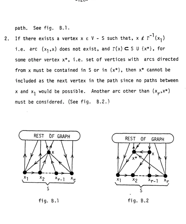
opygI)O'T R09tVE

FL Co '.. 021

39

33.412,

ALGORITHMIC APPROACHES TO

CIRCUIT ENUMERATION

PROBLEMS AND APPLICATIONS

AA

Boon Chai Lee

AA

FTL REPORT R82-7

ALGORITHMIC APPROACHES TO CIRCUIT ENUMERATION PROBLEMS AND APPLICATIONS

Boon Chai Lee

by

BOON CHAI LEE

B.S., University of Michigan (1978)

SUBMITTED TO THE DEPARTMENT OF AERONAUTICS AND ASTRONAUTICS IN PARTIAL FULFILLMENT OF THE

REQUIREMENTS OF THE DEGREE OF

MASTER OF SCIENCE IN AERONAUTICS AND ASTRONAUTICS

at the

MASSACHUSETTS INSTITUTE fF TECHNOLOGY June 1982

Q

Boon Chai Lee 1982

The author hereby grants to M.I.T. permission to reproduce and to distribute copies of this thesis document in whole or in part.

Signature of Author

Department of'Aeronautics and Astronatics

May 7, 1982 Certified by Robert W. Simpson Thesis Supervisor Accepted by Harold Y. Wachman Chairman, Departmental Graduate Committee

ALGORITHMIC APPROACHES TO CIRCUIT ENUMERATION PROBLEMS AND APPLICATIONS

by

BOON CHAI LEE

Submitted to the Department of Aeronautics and Astronautics on May 7, 1982 in partial fulfillment of the

requirements for the Degree of Master of Science in Aeronautics and Astronautics

ABSTRACT

A review of methods of enumerating elementary cycles and circuits is presented. For the directed planar graph, a geometric view of circuit generation is introduced making use of the properties of dual graphs. Given the set of elementary cycles or circuits, a particular algorithm is recommended to generate all simple circuits. A simple example accompanies each of the methods discussed. Some methods of

reducing the size of the graph but maintaining all circuits are

introduced. Worst-case bounds on computational time and space are also given.

The problem of enumerating elementary circuits whose cost is less than a certain fixed cost is solved by modifying an existing algorithm. The cost of a circuit is the sum of the cost of the arcs forming the circuit where arc costs are not restricted to be positive. Applications of circuits with particular properties are suggested.

Thesis Supervisor: Robert W. Simpson

ACKNOWLEDEMENTS

Professor Simpson had been most helpful with his comments and directions throughout the duration of this thesis. He is also always willing to share his invaluable time for discussions. He helped me

present my thesis clearer and better and showed interest in this work throughout. I owe much to him for his gentleness and generousity.

My stay here in the United States was possible from the support of my family. They have been very generous and loving and I missed them

alot. I am very grateful that they have provided me with the chance not

only to further my education but also to introduce me to such a variety of people and habits that continues to entreat me even now.

Next, I would like to thank Yutaka Takase for the excellent

diagrams he drew for me, and to Wu, Yiren and Hirofunii Matsuo for countless hours of interesting discussions.

Joanne Clark also helped with proof reading this thesis

and showed much patience.

This thesis was completed with the help also of Debbi who spent several beautiful Spring days typing.

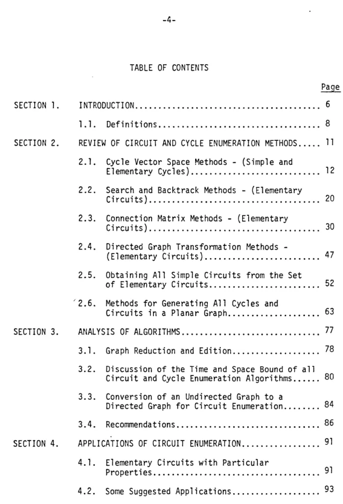
TABLE OF CONTENTS SECTION 1. SECTION 2. SECTION 3. SECTION 4. Page INTRODUCTION... 6 1.1. Definitions... 8 REVIEW OF CIRCUIT AND CYCLE ENUMERATION METHODS... 11 2.1. Cycle Vector Space Methods - (Simple and

Elementary Cycles)... 12 2.2. Search and Backtrack Methods - (Elementary

Circuits)... 20 2.3. Connection Matrix Methods - (Elementary

Circuits)... 30 2.4. Directed Graph Transformation Methods

-(Elementary Circuits)... 47 2.5. Obtaining All Simple Circuits from the Set

of Elementary Circuits... 52 2.6. Methods for Generating All Cycles and

Circuits in a Planar Graph... 63 ANALYSIS OF ALGORITHMS... 77 3.1. Graph Reduction and Edition... .. 78 3.2. Discussion of the Time and Space Bound of all

Circuit and Cycle Enumeration Algorithms... 80 3.3. Conversion of an Undirected Graph to a

Directed Graph for Circuit Enumeration... 84 3.4. Recommendations... 86 APPLICATIONS OF CIRCUIT ENUMERATION... 91 4.1. Elementary Circuits with Particular

Properties... 91 4.2. Some Suggested Applications... 93

SECTION 5. FOOTNOTES.... APPENDIX A. APPENDIX B. REFERENCES... BIBLIOGRAPHY. SUMMARY... ... ...0... ... ... ... 0...0...0....0... .

METHODS FOR FINDING STRONG COMPONENTS

(Christofides [7])... EULERIAN AND HAMILTONIAN CIRCUITS AND CYCLES... Bl. Enumeration of Hamiltonian Circuits Using

the Algebraic Approach: An Example

(Christofides [7])... B2. Enumeration of Hamiltonian Circuit Using

Enumerative Procedure: An Example

(Christofides [7])... ... 0...0... ... ...0...0....0... ... ... &...0....&... Page 104 107 121 126 129 132

Section 1

Introduction

The circuit enumeration problem is of theoretical as well as practical interest. In the past years, we have seen a wide range of

researchers from many disciplines working on this topic. These areas include, Mathematics [3], Computer Science [1,18,34,32], Medicine [25], Transportation [9,21], and Engineering [19,36]. The reason is that many

problems can be represented as graphs. Furthermore, many problems have a cyclic structure where the problem is to identify some or all of the circuits or cycles in the graph.

In particular, this thesis addresses the problem of finding all elementary circuits and cycles in a graph and suggests some related

applications. The areas we will be covering are represented in fig. 1.1. In Section 2, we create four classes of methods of generating

elementary circuits. Every algorithm for generating elementary circuits known thus far, belongs to one of the four methods; namely, the Cycle Vector Space Methods; the Search and Backtrack Methods; the Connection Matrix Methods, and the Directed Graph Transformation Methods. In addition, we provide 6n algorithm for generating all simple cycles or circuits given the set of all elementary cycles or circuits. If the directed graph is planar, we introduce a method for enumerating all the elementary circuits using the dual graphs.

fig. 1.1 Structured approach to generating all cycles or circuits and applications.

enumeration. Before comparing algorithms, the graphs are edited and reduced. Several ways of reducing and editing graphs are given. There-after, the running time and storage requirement of each algorithm is given followed by a short discussion, and recommendations for the best algorithms.

Since complete elementary circuit enumeration problems are known to be difficult and intractable, we have, in section 4, identified a list of circuits with particular properties which, honefully, greatly reduces the number of circuits to be enumerated, followed by some suggested applications that fit into our problem classification. An example would be finding all elementary circuits that do not exceed a certain fixed cost. (The cost of a circuit is the sum of the cost of all arcs in that circuit).

In the final section, we summarize what we have done, and point to some interesting areas of research.

For completion, we have included Appendices to find "strong components" of a graph and a treatment of the problems of finding Eulerian and

Hamiltonian circuits.

1.1 Definitions

The terminologies used in graph theory have hitherto remained at the discretion of the writer. Some writers choose an arc over an edge, a link over a line, or a path over a chain, etc. Furthermore, there have been additions to the glossary of terms used; for instance with flowers, came blossoms, with spanning tree, came forest. Then there are branches

and fronds and twigs, and so forth. As a result, there is a need in this subsection to define certain terms that will be used throughout this thesis. Many ambiguities would be clarified if the reader would take a minute to browse through this subsection.

A graph G(V,E) is defined as a finite set of vertices V and edges E which connects pairs of vertices. The number of vertices IV|=n and

edges IEj=e for a graph G(V,E). A directed graph has arcs which are edges with directions associated with them. A directed graph is more commonly represented by G(V,r) where V is the set of vertices and P is the vertex operator, where for iEV, jEV, jE."(i) if an arc ij exists. Two vertices are said to be adjacent if they are connected by a common edge. Two edges with a common vertex are said to be adjacent.

A path is a directed or undirected sequence of edges or arcs where the final vertex of one is the initial vertex of the next edge or arc. A simple path is a path which does not use the same edge or arc more than once. A simple cycle is a simple path where the initial and final vertex coincide, and the edges contained in the path are assumed to be undirected. A circuit is a directed version of a cycle. An elementary path is a path which does not use the same vertex more than once. An elementary cycle is an elementary path where the initial and final vertex coincide. An elementary circuit is a directed version of an elementary cycle. All elementary paths and cycles or circuits also must be simple. Two elementary cycles or circuits are distinct if one is not a cyclic permutation of the other. We refer to cycles or circuits that are

In this work, we will not be concerned with infinite cycles or circuits.

The length or cardinality of a path, cycle or circuit is the number of edges or arcs appearing in it. A path of length k is called a k-path. The same applies to cycles or circuits.

For a directed graph, the indegree and outdegree of a vertex is the number of arcs terminating and originating at that vertex. The degree of a vertex in an undirected graph is the number of arcs incident to it.

A vertex i is connected to

j

if there exists a path from i to j. A connected undirected graph is one for which a path exists between every pair of vertices. Similarly, a directed graph is connected if its

associated undirected graph is connected. Note there may not be a direct path connecting all vertices in a directed graph. In our work, we shall only be concerned with connected graphs.

A subgraphG(X,A) of a graph G(V,E) is a graph such that X C V and A C-E. A tree of an undirected graph is a connected subgraph which has n

cycles. A spanning tree of a graph is a tree of the graph that contains all the vertices.

Any other definitions that are necessary will be introduced subsequently.

ed

Section 2

Review of Circuit and Cycle Enumeration Methods

This section reviews the different methods for generation of the elementary cycles/circuits in a graph. All algorithms known thus far for enumerating elementary cycles/circuits can be classified into one of the following methods:

2.1 Cycle Vector Space Methods. 2.2 Search and Backtrack Methods. 2.3 Connection Mlatrix Methods.

2.4 Directed Graph Transformation Methods.

The purpose here is to explore the underlying idea behind each of these methods by referring to explicit algorithms.

Thereafter, we examine procedures for generation of all. the simple circuits

in a graph given the set of elementary circuits. An easy procedure to do this is recommended.

Due to close associations of the Travelling Salesman and the Chinese Postman Problem to the Hamiltonian and Eulerian circuit generation, we have included a rather complete discussion on the enumeration of

Hamiltonian and Eulecian circuits in Appendix B. We have not included the discussion in this section in order to reduce the amount of redundancy since the enumeration of Hamiltonian and Eulecian circuits are special cases of the cycle/circuit enumeration methods we will be dealing with

Finally, this section concludes by introducing a method of generating all elementary circuits in a directed planar graph using vertex aggregation of the associated dual graph.

2.1 Cycle Vector Space Methods

These methods apply to an undirected graph and finds all elementary and/or simple cycles. Given an undirected graph G(V,E), a spanning tree Tg is first constructed having n-l edges. Tg is not unique. The addition to Tg of any edge in G (but not in Tg) will form a unique elementary

cycle. Every cycle formed in this way contains at least one edge not found in another. The set of cycles formed by adding all edges in G (but not in Tg) provides a basis for the vector space of all the simple cycles in the graph. Since there are e edges in G and n-l edges in Tg, the number of such cycles that will be formed is e-n+l. This is the cyclomatic number of G, v(G). The v(G) cycles formed in this way are known as a fundamental set of cycles

The derivation of the fundamental set of cycles is not difficult and therefore, the reader is referred to Gotlieb and Corneil [15], Welch [36] or Paton [25] for an algorithm for finding the fundamental set of cycles. The algorithm of Gotlieb and Corneil [15] is slower than that of Welch [36] but requires less storage for graphs with a large number of vertices.

The algorithm of Paton [25] on the other hand is compatible to Gotlieb and Corneil [15] in terms of storage and to Welch [36] in terms of speed. The author recommends the algorithm of Paton for finding the fundamental set of cycles.

Since the fundamental set of cycles is a basis of the vector space for cycles, then any cycle in G not in D, can be formed by a linear combination of cycles in (_ by the following convention.

Let every fundamental cycle 4)i, i=1,2,...v(G),be represented by an e dimensional vecter where the jth element is 1 if the jth edge is part of the cycle, and zero otherwise. The ring sum operation can be expressed for vectors A and B as A + B= {xJxcAUB,AfB}. If the ring sum, @ ,is used

for mod 2 addition, any cycles in G not in , can be expressed as a ring sum operation of fundamental cycle. The ring sum of 2 cycles is a cycle or an edge disjoint union of cycles.I The edge disjoint union of cycles means the union of cycles having no common edges. To generate all the cycles in G, we need to consider all 2v (G)-v(G)-I combinations of

fundamental cycles. However, some of the combinations will be disjoint cycles, but, if a given combination is disjoint one cannot disregard other combinations containing it since the mod 2 addition of it and another combination might produce a single cycle. Thus, one can simply enumerate all possible cycles in the graph using this property of the fundamental set of cycles found by selecting a spanning tree.

Gibbs [14] presented a corrected version of Welch's algorithm to generate all the elementary cycles in the graph. The algorithm is

presented here as ALGORITHM 1 for completion.

We note that the set R generally remains smaller than Q which contains all the linear combinations of fundamental cycles at the end. This is more suitable for programming.

ALGORITHM 1. GIBB's algorithm for generating all elementary cycles from the fundamental set of cycles.

Given a set of fundamental cycles 4 = { #1, 02, . u(G)

1. Set S = {01_{}, Q = {01}, R = 0, R* = 0, i = 2.} 2. For all T in Q,

If T i ? f 0 place T

*

Oc into R,

If T 0 (D 0 place T $ @. into R*.

3. For all U and V in R, if U C V set R = R - { V}

and R* = R* U { V}. 4. Set S = S U R U { D }.

5. Set Q Q U R U R*U{ . Reset R =0

;

Reset R* =0.

6. Set i = i + 1. If i < u(G), go to 2. If i > u(G), STOP; S consists of all the elemenatary cycles in the graph.

Note: T is any element of Q, i.e., it could be a cycle or an edge disjoint union of cycles.

Methods.

Given: G,

We obtain the fundamental

i : Adding edge 1 3 : Adding edge 5 4 set of cycles :-)2 : Adding edge 3 04 : Adding edge 8

2

13

5 16

7 8 G 1 l 1 0 1 0 0 0 0 02 0 1 1 1 0 0 0 0 G2 0 0 0 1 1 1 0 0 oD 4 0 0 0 0 0 1 1 1

algorithm:

Iteraion Results Action

1 S =1, Q=4)i, R =, R*=$ (STEP 1) 2 01n 02

0

Z => R = 01 0 4)2 (STEP 2) 3 S = 41, '01 e 4)2, )3 (STEP 4) 4 Q = 014,41 * 02, '₂, R = 0, R*=

0

(STEP 5) 5 i = 3, 3 < U(G) = 4 (STEP 6) 6 D1 (1 3

#

0 (41 0 42 ) (103 =0 R= 0IG43, 02 0 3 (STEP 2) 0 2 4'3

#

R* = $1 0 $2 (D 3 7 S = $I, (De 1 2, (D1 (3, (2 )3 3 (STEP 4) 8 Q = 1 i, ' 1 e *2, 42, 01 1 3, (DI 1'2 P3, 02 1 (D3, 03. (STEP 5) R =0, R*=0. 9 i = 4, 4 < u(G) = 4 (STEP 6) 10

₄₁

_{lA (#4 /,} 2 1 4 ) = 0, (1 * 't2)f)( 4 0, (1 i 4 2 * 43) A4 #4 , (01 15 # 3)(104 A 0, ((D2 S 'D3) 4 _, D3 () 44 1 0. _{(STEP 2)} => R =

{

$1 (D ( 3 a 4, i) G 4)2 N 4, (D 2 $ 4) 3 4)4, 4)3 0 '44 R* = D 4) , (D - #P2 44, (2 4)4

11 In this case, we enter step 3,

(D3 S 4 CD 1 4 )2 9 '3 4 since (0 0 0 1 1 0 1 1) (1 0 1 1 1 0 1 1 ) i.e. (1 0 1 0 0 0 0 0 )U (0 0 0 1 1 0 1 1), therefore, (STEP 3) R = { #1 e #)3 4 44, 2 D3 *4) 4, 4)3 $ 4) R* = { i 4, $1 4)2 S 4, (D2 44, 1)1 02 t )3 0 4)4 1

Iteration Results Act ion 12 S = $1, *i D 1 2, D2, '1'S i 3, 9 '2 f 'D3' _{(STEP 4)} 43, (i I t 3 e 4, 4 2 1 ( 3 (D4, (3 e 4)4, 24. (STEP 5) D3 (D e 9 01 4, (D1 e 2 4, * D2 (D4, 1D 4 +2 4)*3 4) 9 4, )4 R = 0, R* =

14 i = 5 5 > U(G) = 4. STOP. (STEP 6)

S in iteration 12 contains all the elementary cycles in the graph, and Q in 13 all the linear combinations of the fundamental cycles.

Example 1 illustrates the enumeration of all elementary cycles from the fundamental set of cycles. However, the set of fundamental cycle forms a basis for all the simple cycles of the graph as well. These simple but non-elementary cycles can be found in set Q. One way of obtaining these will be discussed in section 2.5.

Thus far, we have restricted our discussion to an undirected graph only. For a directed graph, there are no equivalent fundamental sets of circuits. Under the ring sum operation, + , cycles and edge disjoint union of cycles in the undirected graph form a group. Every element of this group can be expressed as a ring sum of some of the fundamental cycles with respect to a spanning tree. However, there exists no binary operation under which all circuits and edge disjoing unions of circuits

form a group, let alone a vecter space. (Narsingh Deo [10]). Cycle Vector Space Methods are not applicable to a directed graph.

We note from the above discussion that the fundamental set of cycles is central to cycle enumeration. In the discussion following we point out two interesting relationships between the fundamental cycle matrix and the cutset and incidence matrix. These relationships not only offer better insight into the properties of the fundamental cycle set but also application to other seemingly unrelated problems. A few definitions are necessary before we proceed. The fundamental cutset2 matrix is defined as an (n-1) x e matrix K = [ki1] where kj = 1 if edge

j

is part of

as an n x e matrix B = [bij] where bij = 1 if vertex i is incident to edge

j

and zero otherwise. We state the two relationships under theorems one and two.

Theorem 1. The incidence matrix B and the transpose of the

fundamental cycle matrix PT are orthogonal, i.e.,B-.T =O. Theorem 2. The fundamental cycle matrix 4_ and the cutset

matrix KT are also orthogonal, i.e., D-KT = 0. The two theorems can be shown easily by observing

that:-1. Each vertex in a cycle is incident with an even number of edges in the cycle.

2. Each cycle cut by a cutset has an even number of edges in common with the cutset.

Observe that all operations are done in mod. 2. Moveover, the theorems are valid for any cycle and cutset matrices defined so long as matrix multiplication rule is not violated. The fundamental cycle set

have been used to solve electrical circuit problems (see Christofides [7]). In addition, from the max-flow-min-cut theorem for the maximum flow problem, one would search for the min-cut by observing the

relationship between the fundamental cycles and the fundamental cutsets. Note that this orthogonality relationship extends beyond the fundamental sets to include all the cycles and cutsets in any given graph.

One of the drawbacks of the Cycle Vector Space Methods stem from the fact that in most cases, the ratio of the number of nondegenerate or valid cycles to the number of vectors goes asymptotically to zero

as the number of vertices in the graph increases. The number of

vertices in the graph increases. The number of vectors is 2 )(G)- u(G) - 1

(excluding the basic cycles and the null elements). The ring sum,

*,

taken on combinations of fundamental cycles thus produces many

degenerate cycles or edge disjoint unions of cycles. In fact, it is

shown in Mateti and Deo [23] that there are only four graphs having all 2v(G) - 1 cycles, that is, every combination of fundamental cycles

produces a distinct cycle.

Algorithms which make use of this method were given by Welch [36], Gibbs [14], Mateti and Deo [23], Maxwell and Reed [24], and Hsu and Honkanen [17]. The discussion above attempts to capture the essence of the Cycle Vector Space Methods.

2.2. Search and Backtrack Methods

The search and backtrack method applies to a directed graph only. One such algorithm is presented here to introduce the main idea behind the Search and Backtrack Methods.

The vertices of a directed graph are numbered 1 to JVI = n. The algorithm generates all elementary paths P - {P(1),P(2),P(3),...P(k)} where P(i) is the ith vertex in the k-path P and P(1) < P(i) for all 2 < i < k by starting from an arbitrary vertex P(l), choosing an arc to extend to another vertex P(2) > P(l), and continuing in this way. If the path cannot be extended any further, the procedure backs up one vertex and chooses to extend to a different vertex. If P() is

adjacent to P(k), the algorithm lists an elementary circuit

(P(l),P(2),... ,P(k),P(l)). This algorithm enumerates each elementary circuit exactly once, since each circuit contains a unique "initial vertex," P(O), and thus corresponds to a unique elementary path

starting from that vertex.

Given a directed graph, we first reduce the size of the graph by eliminating vertices which cannot belong to any circuits. The process is to remove any vertices on which no arcs terminate and all arcs originating from these vertices. Similarly, all vertices in which no arc originates, and any arcs terminating on these vertices are also removed. This step is repeated until no such vertices remain. Then, k parallel arcs are reduced to a single arc, but k circuits are later listed if that particular arc forms part of any circuit. More

discussions on graph reduction will appear in Section 3.1. The reduced directed subgraph G(V,r) is defined as a set of vertices V = (1,2,...n) and an arc operator r(-) which operates on all elements of V; j c r(i) if there exists an arc from i to

j.

Graph G(V,r) is an n x n array G(i,j) (see Example 2).

The algorithm assigns integer values, 1,2,...,n to each of the vertices in G. It utilizes two principal arrays in addition to G(i,j). The first,

P, is an n x 1 array, containing all the vertices in an elementary path.

The second is an nx n array, H, which is initially zeroed. H contains the list of vertices "closed", to each vertex. Vertex j is "closed" to i when-ever an arc from i to

j

has been previously considered. The algorithm

basically involves elementary path building in array, P. We can now explain the algorithmic process.

Search

Starting from an- "initial" vertex 1, a path is extended from its end, one arc at a time such

that:-a. The extension vertex cannot be already in P.

b. The extension vertex value must be larger than the initial vertex.

c. The extension vertex is not "closed" to the last vertex in P. H contains the list of vertices closed to each vertex.

(Vertex closure will be discussed further under (Backtrack).)

(a) assures that an elementary path is being considered. (b) assures that each circuit will be considered only once. (c) assures that each elementary path is considered only once.

At some point, no vertices will be available for extension. We test for a circuit by seeing whether there is an arc connecting the last vertex of P to the first vertex. If there is, then a circuit is reported. In any case, vertex closure occurs unless there is only one vertex remaining in the path.P.

Backtrack

Vertex closure consists of three steps:

1. Enter the last vertex of P into the list in H for the next to the last vertex in P.

2. Clear the list in H for the last vertex.

3. Shorten P by one arc by eliminating the last vertex.

(1) assures that the path extension just performed will not be repeated. (2) allows correct forward continuation from the last vertex if it is reached by a different path in the future.

The extension and backtracking continues until the path has been backed to the "initial" vertex 1. Then, the "initial" vertex is advanced. This means that the first vertex is incremented by one;

H is cleared; and the extension process resumes. No paths, and thus circuits containino vertex 1 will be considered again. All circuits containing vertex 1 will have been found. The algorithm

continues to extend paths and advance the "initial" vertex sequentially until P contains a path of one vertex, namely, vertex n. At this

point, the algorithm terminates. All elementary circuits have been identified.

The algorithm discussed above, and the exact algorithm presented in ALGORITHM 2 is attributed to Tiernan [34]. Example 2 illustrates Tiernan's algorithm.

The author selected this algorithm by Tiernan [34] to introduce the fundamental idea behind the Search and Backtrack Methods because of its simplicity in exposition, and also because all the other Search and Backtrack Methods develop upon the main idea that was introduced by this algorithm. In Section 4.2., we will show how some slight modifications of Tiernan's algorithm solves a specific problem. In

ALGORITHM 2: An Algorithm for Enumerating all _{Elementary Circuits in} the Graph (Tiernan)

Bl. Initialize Read N,G

P

+

0

H

+0

k

+

1

P() + 1. B2. Path Extension

Search G(P(k,j) for

j

= 1,2,...N such that the following three conditions are satisfied:

(1) G(P(k),j) > P(l) (2) G(P(k),j) I P

m = l,2,...N. If this j is found, extend the path,

k

-+- k + 1

P(k) + G(P(k - 1),j) go to B2.

If _{no j meets the above conditions, the path cannot be extended.}

B3. Circuit Confirmation

If P(1) i G(P(k),j), j = 1,2,...N then no circuit has been formed,

go to B4.

Otherwise a circuit is reported, Print P.

B4. Vertex Closure

If K = 1, then all of the circuits containing vertex P(1) has been considered.

o to B5. Otherwise,

H(P(k),m) +- 0, m = 1,2,...N

For m such that H(P(k - 1),m) is the leftmost zero in the

P(K - 1) - the row of H, H(P(k - 1),m) +- P(k) P(k) +- 0

k

+- k -

1

go to B2.

B5. Advance Initial Vertex If P(l) = N then-go to B6.

otherwise, P(l) - P(1) + 1

k

+1

H

+0 go to B2.

B6. Terminate

Example 2.Circuit Enumeration using Tiernan's algorithm presented in ALGORITHM 2. 2 1 2 0 0 0 3 0 0 0 0 3 G (V,') = 1 2 3 4 0 5 0 0 0 0 1 3 0 0 0 5 4

Note: The parallel arcs (5,1) have been replaced by a single arc (5,1).

P ACTIONS ON ATTAINED PATH

1 0 0 0 0 -81. Initialization. 1 2 0 0 0 B2. Path extension. 1 2 3 0 0 B2. Path extension. 1 2 3 4 0 B2. Path extension.

1 2 3 4 5 B2. No path extension. B3. Circuit reported, (1 2 3 4 5 1). B4. Backtrack and vertex closure, H(4,1)<--5.

1 2 3 4 0 B2. No extension. B3. No circuit formed.

B4. Clear last vertex, H(4,1)<--O, Backtrack and vertex closure H(3,1)<--4

1 2 3 0 0 B2. No extension. B3. Circuit reported, (1 2 3 1) B4. Clear the last vertex, H(3,1)<--O, Backtrack and vertex closure, H(2,1)<--3.

1 2 0 0 0 B2. No extension. B3. No circuit.

84. Clear last vertex, H(2,1)<--O, Backtrack and vertex closure H(1,1)<--2

1 0 0 0 0 B2. No extension. B3. Circuit reported, (1 1) B4. Cannot backtrack. B5. Advance vertex, i.e. set P(1) = 2, Clear H.

Comment: All circuits containing vertex 1 have been enumerated.

2 0 0 0 0 B2. Path extension. 2 3 0 0 0 B2. Path extension. 2 3 4 0 0 B2. Path extension.

2 3 4 5 0 82. No path extension. 83. No circuit found. B4. Backtrack and vertex closure, H(4,1)<--5.

2 3 0 0 0 2 0 0 0 0 0 0 0 4 0 0 4 5 0 3 4 0 0 0 3 0 0 0 0 4 0 0 0 0 4 5 0 0 0 4 0 0 0 0 5 0 0 0 0

last vertex, H(4,1)<--0, Backtrack and vertex closure, H(3,1)<--4.

B2. No path extension. B3. Circuit formed, (2 3 2) B4. Clear last vertex, H(3,1)<--0, Backtrack and-vertex closure H(2,1)<--3.

B2. No path extension. B3. No circuit formed. B4..Cannot Backtrack. B5. Advance vertex, i.e. set P(1) = 3. Clear H.

Comment: No circuit formed hereafter would contain vertices 1 or 2.

B2. Path extension. B2. Path extension.

B2. No path extension. B3. Circuit reported, (3 4 5 3). B4. Backtrack and vertex closure, H(4,1)<--5.

B2. No path extension. B3. No circuit reported.

B4. Clear last vertex H(4,1)<--0, Backtrack and vertex closure H(3,1)<--4.

B2. No path extension. B3. Circuit reported, (3 3). B4. Cannot Backtrack. 85. Advance vertex, i.e. set

P(1) = 4. Clear H.

Comment: No circuits formed hereafter would contain

vertices 1, 2 or 3. B2. Path extension.

32. No path extension. B3. No circuit found. B4. Backtrack and vertex closure, H(4,1)<--5.

B2. No path extension. B3. No circuit formed. 84. Cannot Backtrack. 85. Advance vertex, i.e. set P(1) = 5, Clear H. Comment: No circuit formed hereafter would contain

vertices 1, 2, 3 or 4.

B2. No extension possible. B3. No circuit formed. B4. Cannot Backtrack; all circuits containing P(i) = 5 have been found.

B6. Since P(1) =5; Terminate.

Comment: All circuits in the graph have been found.

Circuits founded

are:-2 1-circuits(self-loops), (1 1) and (3 3) 1 2-circuit, (2 3 2)

2 _{3-circuits, (1 2 3 1) and (3 4 5 3)} 2 5-circuits, (1 2 3 4 5 1 )

the discussions following, some similar methods are highlighted. An example provided by Tarjan [32] shows the inefficiency of the above algorithm in the worst case. Weinblatt [35] provides an

algorithm that examines each arc of the graph only once. He uses a recursive backtracking procedure to test combinations of subpaths from old circuits to see if they result in new ones. Tarjan [32], however, showed also that Weinblatt's algorithm does not have a running time polynomial to the number of circuits in the given graph.

Taijan [32] uses Tiernan's backtracking procedure but also uses a marking procedure to avoid unnecessary searches which help decrease the size of the subset of paths that need to be generated considerably. The running time of Tarjan's algorithm is shown to be polynomial to the number of, circuits in the graph.

Johnson [18] and Szwarcfiter and Lauer [31] use improved pruning methods over 'Tarjan's [32]. Their alaorithms have running times that

are also polynomial to the number of circuits in the graph, but are an improvement over Tarjan's. In particular, Johnson's [18] algorithm is shown to be asymptotically fastest (for a large graph).

The algorithms of Char [5] and Chan and Chang [4] use the set of all permutations of vertices of the graph as the search space. Other algorithms using the Search and Backtrack Methods have also been

presented by Berztiss [2], Roberts and Flores [29], Reed and Taijan [28] and Ehrenfeucht et al. [12].

2.3. Connection Matrix Methods

These methods make use of the properties of the connection matrix

of a directed graph to generate elementary paths as vertex sequences. In _{our generation of elementary paths however, we would also be} generating simple and non-simple paths.3 The method eliminates all simple (but non elementary) and non-simple paths as soon as they are formed. It builds elementary paths one arc at a time and lists circuits for each cardinality in increasing order.

Before proceeding to discuss the method, a simple but important theorem is given. This theorem establishes the fundamental idea behind the Connection Matrix Method. We state the theorem for the

adja-cency matrix, - but the idea can be easily extended to connection

matrix since the difference between the adjacency and connection matrix is that the ij elements of the adjacency matrix are ones or

zeros depending on whether arc ij exists whereas theij elements in

the connection matrix tells us the number of arcs from vertex i to

j,

A directed graph can be represented as an n x n adjacency matrix, A = [(a)..] where (a)i. = 1 if arc ij exists and zero otherwise. Only self loops would appear as a non zero element in the diagonal of A. We state the theorem formally:

Theorem 3: The ij element of Ak is the number of paths of length k, or "k-paths" from i to

j.

If a k-circuit (that is, of cardinality k) exists, there would be a non-zero element in the diagonal of the Ak matrix. However, a non zero element in the diagonal does not mean that a simple k circuit exists. The reason for this is that when we take the product of the adjacency matrices, infinite paths and/or circuits (that uses one or more arcs repeatedly) are formed. One could extend this result to the connection matrix, that is, the ij element for the matrix C1 (where C1 is the connection matrix) equal to the number of paths of length k from vertex i to j.

A method to resolve the problem outlined above is suggested by Kamae [19]. This method breaks up circuit generation into three stages: (1) path enumeration, (2) flower enumeration and (3) circuit enumeration. We now proceed to discuss this method in more detail.

Define a connection matrix C1 = [(cl)ij] of a directed graph G such that the ij element, (c ) equals to the number of arcs from i to

j

in G.4 (Note that C1 is similar to the adjacency matrix if there are no parallel arcs in G.) Next, define C j as a matrix where,

(ci) = (c1)ij if i / j

= 0 for i =

j,

where i,j = 1,2,...n

Then, let C2 = C - Ci = (C')2 which means that each non zero element in C2 indicates the number of 2-paths or 2-circuits. Next, let C be the matrix C2 with no 2-circuits, i.e.,

(cs) = 0 if i = j

= (c2) ij otherwise

then, consider the matrix multiplication C - Ci where the elements

are:-n

(c - cj). ₁₃ = _{k= 1} (ci)ik (cjkj

Given these elements, we will generate elementary paths, circuits and flowers. Suppose i / j, i / k and

j

/ k, we have two cases:

Case 1

intermediate points

on 3-path from i to

j.

Case 2

Whenever i = k or

j

= k, (c)ik - (ci)kj = 0, thus i / j implies that (C - Ci)ij is equal to the number of 3-paths and 3-flowers from i to j. Next, suppose i = j, then ( Ci)ij equals to the number of 3-circuits containing i.

The method by Kamae [19], for more general cases is stated is stated in ALGORITHM 3.

Since all circuits must be of length lesser or equal to n, we need to compute only up to matrix Zn*

We shall work on the same graph as used in section 2.2. to illustrate the method that was discussed in Example 3.

At this point, we can make several observations. Note that there is more than one way of obtaining the h-path connection matrix. We have merely illustrated one way of doing so in our example. Kamae's method chooses to eliminate non simple paths as the algorithm proceeds instead of sorting paths at various points in the algorithm. Due to this, Kamae's method is more favorable for computer implementation.

In general, different Connection Matrix Methods differ only in the way they avoid generating the arc or vertex sequences that can neither belong to paths nor circuits, i.e. non simple or infinite arc sequences.

Other algorithms that belong to this class can be found in Ponstein [26], Yau [37], Danielson [8] and Ardon and Malik [1]. In particular, Ardon and Malik reduce the storage bound to 0(n2_{) by} finding circuits, using Boolean reduction, to an expression which

ALGORITHM 3: Kamae's Algorithm for Generating All Elementary Circuits Using Connection Matrix Method.

1. Path Enumeration

Def. 1. The element of an h-path connection matrix, Ch, of G is defined by:

(ch)ij = number of h-paths from i to

j

if i

/

j

= number of h elementary circuits containing i if i = j.

Def. 2. A proper h-path connection matrix CG of G is defined by:

(c ) = (ch)ij if i

= 0 if i =j

Def. 3. Let L be the set of all (h-t)-circuits and y be a particular (h-t)-circuit belonging to set L. Then, an

(h-t) flower matrix Ch3t of G is defined by,

Ch,t = C (ht) , t > 1, h - t > 2

where (cy(hqt) )ij equals the number of t-paths from i to j which do not touch y1 except at j if i y and j c p, and

zero otherwise.

An (h,t)-flower is an h-flower which contains a t-path and an

(h-t)-circuit with only one vertex in common, that is the joint. Cy(ht) then represents all (h,t)-flowers which contains y, since a

flower from i to j consists of a circuit i containing j and a path from

i to j not touching y except at j. Chst as defined above, is then the sum of Cu h,t) over all (h-t)-circuits, (ch,t)ij then equals to the number of (h,t)-flowers from i to j where j is the joint.

With this backtround, we are now able to state a theorem for Ch

(The connection matrix which counts h-paths and h-circuits). Theorem 4. h-2 Ch C h-1-Cl -I c ht > 3 t=1 h = C -C h = 2 h-2

ICht denotes the sum of the number of (h-t)-flowers where

t=L h

t = 1,...h-2. We are essentially removing all flowers each time we try to find Ch. Note that for h = 2, no flowers can be formed therefore

h-2

the term I Ch t is not needed. t=l

2. Flower Enumeration

Def. 4.

(j)qr =

that is, DI1 is a matrix of the graph G obtained from the connection matrix by deleting all edges incident from vertices contained in circuit p. D1, Dhj _{etc., are defined in parallel with C CG} etc. So with theorem 4 for connection matrices, we have,

Theorem 5: t-2 Dt= D 1 -Di j- Dts t > 3 t - ~ s=1 , D" _t =DI' Dill _{t-l 1} t = 2 t-2

As in theorem 4, 1 Dt s denotes the flowers of length t, with s=l t

circuits of length t-l and less (but not lesser than 2). We next

state another theorem which will be useful for obtaining the number of flowers.

Theorem 6: Recall that - is a (h-t) circuit,

(D) = (c(ht)Iij if i p and j E yp

= 0 otherwise

From definition 4, for i ! 1 and

j

E y, (DI') is the number of t-paths from i to j, not touchina yp except at j (since j has outdegree 0 for the graph defined by D _{'). Note that this corresponds to the} definition of (cy-(ht))ij.(See Def. 3). Hence, (cy,(ht))ij can be determined from DO. This is desirable since by applying definition 5_ta and theorems 5 and 6 repeatedly, we can obtain DU

3. Circuit Generation

After obtaining ch, we would like to be able to list the circuits as vertex sequences. We know that all h-circuits appear as a non zero element in the diagonal of Ch. The following definition will help us.

Def. 5. A h-circuit matrix Zh is defined as,

(zh ij = (c,_ )ji (ci)ij 1 < i, j < n

Notice that since (c'

)

equals to the number of (h-1) paths from

j

to i, and (cj)~ equals the number of arcs from i to j,

(z hij is the number of h-circuits which contains an arc from i to j. The difference between (z h ij and (ch)ij for i =

j,

is that the former provides us with arcs belonging to a h-circuit (that is, a starting point for listing our circuit, whereas the latter just tells us the number of h-circuits containing a certain vertex.

Having obtained Zh, we list the h-circuits by making the first non-zero element in the first non zero row, and list the first arc belonging to the h-circuit. For example, pq, observe that p represents the row and q, the column in which the non-zero element appears. Next, we proceed to the qth row; search for the first (left most) non zero element, and list the next arc in the h-circuit by reading off the corresponding row and column, for instance qr. We proceed in this manner, building an arc at a time until we return to the initial

h arcs. The h-circuit is then pqr...p. In some instances, there might exist more than one h-circuit or more than one that uses the same arc many times. It is then necessary for us to do two

things:-1. After each h-circuit has been listed, we remove all arcs of the h-circuit from the Zh matrix. This is accomplished as

follows:-()i = (zh)ij - 1 V ij belonging to h--circuit listed

= (zh)ij otherwise

The resultant matrix Z contains the remainder of the h-circuits of the graph.

2. We return to our procedure for listing h-circuits until (z) = 0, for all i and j.

---Example 3. Kamae's Algorithm Applied to Circuit Enumeration Results Comments C = C1 = -1 1 0 0 1 1 0 0 2 0 1 0 0 1 1 0 0 0 1 1 0

0-From C1, two 1-circuits, 1,1,3,3

are read off the diagonal

,0 0 1 0 0 1 1 0 1 0 0 0 0 0 1 -2 0 1 0 0-By definition 1. t Ry definition 2. 3. 0 0 1 00 C2 = (C )2 1 1 0 1 0 C2= 0 1 1 0 1 2 0 1 0 0 By definition 1 and 1 3 0 1 0 theorem 4.

Ci'

=

Results

Z

_{2 =} 0 0

0~

1 0 0 0 0 0 0 0 0 0 0 0 From Z 2, a 2-circuit 232 is obtained. Comments From definition 5, (z2)ij = (Cj) -(c') e.g. (z₂)_{2 3} = (ci) _{3 2 -(Cj) 2 3 1} 5.

0 1 0 0~ C is obtained from definition

1 0 0 1 0 _{2. At this point, we have a}

- 0 1 0 0 1

2 -O 1 0 0 one 2-circuit. Let

1 3 0 1 0 y =2-circuit 232.

6.

01 0 00 We obtain D" by eliminating

0 0 0 0 0 _{rows 2 and 3 from C}

1 D = D = 0 0 0 0 0

1 D 0 0 0 0 1 i.e. by definition 4.

Results Comments

7. From D ", we obtain by keeping

0 1 0 0 0 columns 2 and 3, and setting the

0 0 0 0 0 _{remainder columns to zero.}

C = 0 0 0 0 0

C3,1 000(Theorem 6)

0 0 1 0 0 Note: CV(3 1) C3 1 since there is only one 2-circuit.

8. 0 1 0 0 1 C-Cj = 2 0 2 0 0 1 3 0 1 0 0 1 3 0 1 9. From theorem 4, S 0 0 01 _C 3 = ci-C - _C 3,1 C 3 = 2 0 2 0 0 1 3 0 1 0 0 1 2 0 1

Results 10. 0 0 1 0 0 1 0 0 1 0 From z, we obtain the 3-circuits 1231 and 3453.

Comments (z3)ij = (c ) .(cj)

i.e. Definition 5.

Let v be the 3-circuit 1231 and X be the 3-circuit 3453.

11.1

-0 0 0 1 07~ 2 0 0 0 0 1 3 0 0 0 0 1 2 0 0 By definition 2.

12. _{Since v is the 3-circuit 1231,}

0 0 0 0 0~ we obtain D ' by removing rows

0000 ₀ 1,2,3 from C1 . 0 0 0 0 0 0 0 0 0 1 (From theorem 6.) 20 10 0

Z

3 =

C

=

Results C (4 .1) = Comments 0 0 0 0 0 0 0 0 1 0 We obtain cv(4 1 ) by keeping columns 1,2,3, from D . 14. Since A = 3-circuit 3453, 01 ₀ 00 _{we obtain D by removing} D D 0 0 0 0 0 rows 3,4,5 from C 0 0 0 0 0 (Again, Theorem 6)

0 0

0 0

0-15. From D we obtain C 0 0 0 0 07 _{by keeping columns 3,4,5} 0 01 0 0 CA(l)= 0 0 0 0 01 fromD. 0 0 0 0 0 0 0 0 0 0-16. Hence, 0 0 0 0 0~ 0 0 1 0 0 C₄ = Cv 4 1) + C C4 ,1 0 0 0 0 0 0 0 0 0 0

2 0 1 0 0 i.e. from definition 3 and theorem 6.

Results 17. D = D = 22 Comments 07 0 0 0 0 From DU , we obtain D = (Di) -(D") (Theorem 5) 18.

0 0 0 0 0~ Hence, we can find C4,2 from

00000 _{by returning columns 2 and}

C4,2 _{0 0 0 0 0 3} 0 0 1 0 0 3 0 2 0 0 0 19. 2 0 1 0 0 C -C= 0 2 0 0 0

0 1

3 0 0

2 2

1 2

0

20. _{From what has been obtained, we}

2 0 0 0 0 get,

C

4 C4 0 2 0 0 0 C= C' - C

-4 0 1 2 0 0 C4 3 'l 4,1 -C4,2

0 0 0 2 0 j(Theorem ₄₎

C4 = C since diagonal elements of C4 are zero.

Comments

Since there are no 4-circuits.

22.

~~ 0 0 0 0 Now, for 3-circuit v,

0 0 0 0 0

D = D = 0 0 0 0 0 D

2 0 1 0 0 _{(Theorem 5)}

0 0 0 0 0

23.

F0 0 1 0 0 And, for 3-circuit X,

O 0 0 0 0 D A= D = 0 0 0 0 0 D2X = D( DX 0 0 0 0 0 0 0 0 0 0_ (Theorem 5) 24. '0 0 C

5v2

0

C5,2 = 0 2 0 07 0 0 0 01

The same way C451 was obtained. Note however that we are doing this for all 3-circuits now, i.e. v and

X

(left as an exercise). (Theorem 6 and Definition 3)

25. From D and

T~0 0 'O 0 0~

00 00 D11=D _D~ 1'- (TheoremS5)

0 0 0 0 0 _{3 3}

D 0 0 0 0 0 _{Note: D = 0 because D has no}

0 2 0 0 0 de 2

diagonal elements or no 2-circuit.

.'. D3 = D -D 1 Results

Results Comments

From D we obtain C5 3 by

keeping columns 2 and 3 corresponding to 2-circuit p. (y = 2-circuit 2,3,2) (Theorem 6) 27. _{-2 0 0 0 0~ 3} 0 2 0 0 0 C5 = C4 -C - 1 _t=1 C5,t C₅ = 0 0 2 0 0 0 0 0 2 0 (By Theorem 4) 0 0 0 0 2

0o

0 0 2 0

There are two 5-circuits,

both of which are identical, 123451. By definition 5, (zS 5ij = (c4) -o(c )i ************* End of Example 3 * 26. C 593 28.

z

_{5 =}

results from the permanent expansion of matrix M, where M = C + I and C is the variable adjacency matrix and I, the identity matrix. A new expansion, the "pseudopermanent," is defined by which the set of circuits can be formed directly. An extension of the method to find Hamiltonian circuits is also included. The method of Ardon and Malik offers

improvements over all the other Connection Matrix Methods since the storage requirement is O(n2) as opposed to O(n(const)n) for the others. We will mention more about the comparison between algorithms in

Section 3.

2.4. Directed Graph Transformation Method

A directed graph can be transformed into a "line graph" where the properties of the "line graph" are useful for the purpose of circuit enumeration. Given a directed graph G(V,E), where e. e E, the associated "line graph", Q(G),is a graph where each arc in G

represents a vertex in Q and each two adjacent arcs in E form a

e3 G transforms to,

2(G)

The arc set of G is then the vertex set of Q. Each p-path of G will correspond to a (p-1) path in £. However, each p-circuit of G will correspond to a p-circuit in 2. There is a one-to-one correspondence between circuits in G and Q. (See Cartwright and

Gleason [3] for proof.) The elegance of this method is that we will be able to enumerate and delete the circuits in Q without disrupting the cyclic nature of the original graph.

The algorithm lists all self loop first and eliminates them for G. For G, find (G) and enumerate, then delete all arcs which are members of 2-circuits in Q(G). Let the resulting graph subgraph be

G1. We then proceed to find s(G ), enumerate, then delete all 3-circuits. Note that Q(Gl) has only circuits of length greater or equal to 3.

Call the resulting subgraphs G2, find SI(G 2), and so on ... , until

Q(G ) for p< n-2 is empty. Example 4 will illustrate the method more clearly.

The method outlined above relied on the one-to-one correspondence between circuits in G and Q(G). It allows us to remove circuits as they are formed until eventually none are left, at which point the algorithm terminates. Observe that just as is the case of the

Connection Matrix Methods, all circuits of identical cardinality are found simultaneously.

This method is well suited if the majority of the circuits in the graph we are studying have a small cardinality. Alternatively, we might be interested in circuits of a certain (small) cardinality, or circuits that do not exceed a certain cardinality. The reason for this is that whenever circuits are enumerated, they are also

removed, thus the size of the graph is quickly reduced, and

convergence might be faster as well.6 No other method allows us to remove circuits from the graph and test the resulting subgraph

Example 4. Enumeration of circuits using Directed Graph Transformation Method. Iteration 1. Convert G to Q(G) Q(G) List 2-circuit: e3 e4 e3 in (G).

Delete arcs (e₃ ' e₄) and (e4 , e3) from i(G).

The resulting subgraph is known as G Iteration 2.

Transform G1 to Q(GI)

f5 6 7 f5 (e4 e5 e6 e4) in £(G) Delete arcs (f₁ , f₃)9 (f₃ ' f2) (f2 '

and (f₇ , f₅) from Q(G ) The resulting subgraph is now known as G2

Iteration 3.

Transform G2 to Q(G2

(f₅ ' f6' (f₆ f 7)

(EMPTY SET)

2(G2

No 4-circuits are found.

2(G2) = 0. This means that all the circuits have been enumerated.

Circuits found

are:-e_{3 e}

4 e₃

e1 e_{2 e5 el} e₄ e₅ e_{6 e4}

Cartwright and Gleason [3] have proposed a way of listing circuits from the "line graph," after each transformation (and

reduction). However, we could also use the method outlined in Section 2.3 (Kamae's Method) to enumerate circuits of a given cardinality from the "line graph." The problem still remains with manipulating such huge sparse matrices, which would incur huge storage and elaborate computations.

The transformation from a directed graph to a "line graph"

involves a simple logical relationship which could be further exploited. Instead of representing the graph as an adjacency matrix, it could

also be represented by arc listing, or other methods that are less storage incurring. Operations upon arc listings remain difficult and unexplored and point to possible areas of research.

2.5. Obtaining All Simple Circuits from the Set of Elementary Circuits In the preceding subsections, we have confined ourselves to'

enumerating elementary circuits. In this subsection, we shall present an algorithm for generating all simple circuits, given the set of elementary circuits obtained by any one of the methods discussed in _{Sections 2.2 to 2.4. This algorithm is applicable to undirected} graphs as well, where we are interested in finding all the simple cycles. We have taken the initiative here for two main reasons:

i. The enumeration of all simple circuits from the original graph is complex and as a result inefficient. Furthermore, the number of elementary circuits found in a graph would

help us determine whether it would be wise to proceed with the generation of all simple circuits. This is also because

the algorithm that we are about to propose has a worst case time bound related to the number of elementary circuits. ii. In some problems, the set of all simple circuits corresponds

to a feasible set of solutions for those problems. Additional constraints placed on this set of feasible solutions yield the optimum solution, if one exists. A typical problem would be to list the cheapest simple circuit for each given

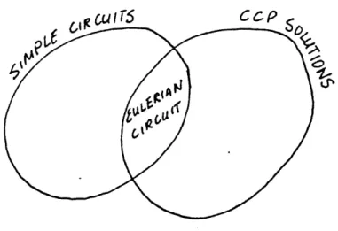
cardinality. After we have obtained this set of simple circuits, we could then use it for dispatching of vehicles. Other examples are best shown by figs. 2.1 and 2.2. Figure 2.1 shows the relationships between simple circuits, elementary circuits and Hamiltonian circuit. It also shows that all solutions to the travelling salesman problem (TSP) are Hamiltonian circuits. In fig. 2.2 , we notice that if an Eulerian circuit exists, it corresponds to the solution for the Chinese postman problem (CPP). An Eulerian circuit is a simple circuit that covers all the arcs in the graph. Note that the solution for the CPP does not have to be simple circuits though. (TSP and CPP are discussed in more detail in Christofides [71.)

fig. 2.1 Relationship between Elementary and Simple Circuits

fig. 2.2 Simple, Eulerian Circuits and CCP

The algorithm which we will present shortly is not meant to solve some of these problems since other methods are available which are more efficient, but rather to illustrate the scope of this endeavor.

The following is an outline of the method:

Let there be q elementary circuits in a given graph defined by Si, where i = 1,2,...q. S. is an e-triple row vector where the jth entry is 1 if the arc j is contained in the circuit, and zero

otherwise. We define _S-.i Sk = $ for 1 < i, k < q if Si and Sk contains no arc in common, otherwise Sinf Sk . Si nSk '

then the S. + Sk will not form a simple cycle. For example, if S = (1,0,0,1), S2 = (1,0,0,0), S₃ = (0,1,1,0), then Sf

A

s2 o and

S1 A S3 2 ( S3 =

o.

(One way to find out is to see if the addition

of two vectors contain any element with value greater than one.) Now, if Sg

A

Sk = $, then Si + Sk would be an arc disjoint union of elementary circuits or a simple but non-elementary circuit. Note however, that if PCA Si = $, where P is a general circuit which may have more than one circuit component. Specifically, P E M, where M = {the set of all arc disjoint unions of elementary circuits or an arc-disjoint union of elementary and simple circuits, or an

arc-disjoint union of simple circuits, or a simple but non-elementary circuit}, then P + S. ' M. To distinguish whether P + Si is a

simple but non-elementary circuit, a few definitions are necessary. We define V(S.) as an n-triple row vector (where n is the total number of vertices in the graph) of circuit S. where the jth entry

(column) is 1 if vertex j belongs to circuit S. and zero otherwise. Next, we define the operation 0 , where: V(P)

0

V(S.) = sum of all positive elements of {(V(P) + V(S)) -

T}; T

is an n-triple vector of ones. This operation defines the number of vertex intersection at P and S _{. We denote also the number of distinct element circuits in P} as xP. For example, let V(Sl) = (1,1,0,1,1), V(S₂) = (0,1,0,0'0)'

V(S3) = (1,1,0,1,0). If P is S1 + S3, then V(P) = V(S1) + V(S3) 8

i.e. x = 2 and S ₌ S2, then,

{(V(P) + V(S₂) -

t}

= (2,3,0,2,1) - (1,1,,,l l) = (1,2,-1,1,0)

and

V(P)

Q

V(S2) = 1 + 2 + 1 = 4

Note that V(P)

()

V(S ₂) > x

.

Now, given that P /A S. = $, if also V(P)

0

V(Si) > x, then P + S. forms a simple but non-elementary circuit. We claim here that if _{xp circuits are joined together such that they do not share any} arc in common and they meet at least x times, then a simple but non-elementary circuit is formed.

If, however, P () S. = $ and V(P) 0 V(S.) < xp, we must not discard P + S. from further comparisons, since the addition of (P _{+ S) and another elementary circuit might form a simple but}

non-elementary circuit. (We store all these in set M in the following ALGORITHM 4.)

But if at any point P11 Si A t, then any further comparisons, that is, additions with P + S. can be eliminated since these

combinations can never form a simple circuit. This elimination rule reduces the possible outcomes we need to consider, which otherwise

would be enormous.

The actual algorithm is presented in ALGORITHM 4.

In order to reduce the number of combinations that need to be considered, it is better to order the circuits in the set of elementary circuits with decreasing cardinality, that is, S1 is the elementary circuit with the highest cardinality, followed by S2' S3' etc. As usual, we include an example to complete our illustration. We refer to the same graph used previously, and reproduced here for convenience in Example 5.

It is important to mention here that in the worst-case the algorithm requires 2q - 1 combinations, where a is the number of

elementary circuits. However, the worst case is highly unlikely

since this would mean that each combination would result in a distinct simple circuit. In that case, by the ordering procedure that we have recommended, the number of combinations that need to be

considered can be reduced. The amount of reduction would depend on the nature of the set of elementary circuits. Even then, this