Coflow scheduling in data center networks

Coflow Scheduling in Data Center Networks

by

Ertem Nusret Tas

Submitted to the Department of Electrical Engineering and Computer

Science

in partial fulfillment of the requirements for the degree of

Master of Engineering in Electrical Engineering and Computer Science

at the

MASSACHUSETTS INSTITUTE OF TECHNOLOGY

September 2019

c

2019 Massachusetts Institute of Technology. All rights reserved.

Author . . . .

Department of Electrical Engineering and Computer Science

July 25, 2019

Certified by . . . .

Eytan H Modiano

Professor

Thesis Supervisor

Accepted by . . . .

Katrina LaCurts

Chair, Master of Engineering Thesis Committee

Coflow Scheduling in Data Center Networks

by

Ertem Nusret Tas

Submitted to the Department of Electrical Engineering and Computer Science on July 25, 2019, in partial fulfillment of the

requirements for the degree of

Master of Engineering in Electrical Engineering and Computer Science

Abstract

In this work, I analyze the problem of coflow scheduling on a multi-stage cross bar switch with a set of intermediate ports. Using a multi-stage abstraction for the data center network enables development of algorithms that reduce the network latency for certain traffic patterns. In this context, I compare the capabilities of the multi-stage network with the cross-bar switch via simulations and theoretical calculations. A theoretical upper bound of 1/e was shown for the ratio of the difference between the minimum total coflow completion times (TCCT) on these two networks and the minimum TCCT on the cross-bar switch. On the other hand, simulations using approximation algorithms gave values of up to 8 percent for the average of the same ratio under randomly generated traffic patterns.

Thesis Supervisor: Eytan H Modiano Title: Professor

Acknowledgments

I would like to thank Professor Eytan Modiano for all his help during my time as a master of engineering student at MIT. I would like to emphasize that besides his guidance regarding the specific aspects of my thesis topic, his efforts to teach ways of academic research and his feedback on my work has been extremely important for equipping me with the necessary skill for a PhD. I also would like to thank my friends in the Communication Networks Research Group for their eagerness to help whenever I faced a problem in my research. Finally, I would like to state that I am glad to have been a part of the LIDS and met all the amazing people in this wonderful community.

Contents

4 Throughput Analysis 31

5 Latency Analysis 33

6 Bounds on the Maximum Improvement Ratio 49

6.1 Lower Bound on the Maximum Improvement Ratios . . . 50 6.2 Upper Bound on the Maximum Improvement Ratios . . . 63

7 Complexity 79

8 Algorithm 81

9 Simulation 95

List of Figures

1-1 A sample blocking DCN architecture [2] . . . 16

1-2 Classical three tiered tree architecture [6] . . . 17

1-3 4 pod fat tree architecture with 16 servers [1] . . . 17

1-4 4-by-4 CBS . . . 18

1-5 4-by-4 Clos . . . 19

5-1 Traffic pattern C on a 4-by-4 Clos . . . 35

6-1 Traffic pattern on an N-by-N Clos . . . 51

6-2 Traffic pattern C on a 10-by-10 Clos . . . 54

9-1 Graph of the competitive ratio averages µ(α8.1), µ(α8.2) and µ(α8.3) with respect to the port ratio r . . . 99

9-2 Graph of the improvement ratio averages µ(IR1) and µ(IR2) with re-spect to the port ratio r . . . 100

List of Tables

5.1 Traffic pattern for example 5.1 . . . 34

5.2 Traffic pattern for example 5.2 . . . 37

5.3 Traffic pattern for example 5.3 . . . 40

5.4 Traffic pattern for example 5.5 . . . 45

9.1 Mean of the parameter values obtained from the simulations on 32-by-32 CBS and Clos . . . 97

9.2 Standard deviation of the parameter values obtained from the simula-tions on 32-by-32 CBS and Clos . . . 98

9.3 Maximum of the parameter values obtained from the simulationa on 32-by-32 CBS and Clos . . . 98

9.4 Minimum of the parameter values obtained from the simulationa on 32-by-32 CBS and Clos . . . 99

Chapter 1

Introduction

Modern data analysis tools such as MapReduce consist of multiple stages of compu-tation, each of which utilizes services of a large number of servers. Hence, transitions between these stages are characterized by large volumes of communication among these servers. For instance, a MapReduce task of m mappers and r reducers requires transmissions of mr and r flows in its shuffle and output replication stages respectively and cannot complete before all of these flows reach their destinations. Generalizing this observation, completion times of each task run on data center networks (DCNs) depend on the completion time of the slowest flow among those scheduled by that task. The recently proposed coflow abstraction aims to capture this property by grouping multiple flows associated with a single task into a coflow whose completion time equals that of the slowest flow in the group. Accordingly, coflow is defined as a collection of flows between two groups of machines with associated semantics and a collective objective [3]. For instance, all of the mr + r flows in the example above constitutes a single coflow which represents the data center traffic associated with that single MapReduce task.

Given the power of coflows in capturing the relation between flows and tasks on DCNs, coflow scheduling becomes an important component of optimizing the DCN performance. While scheduling coflows, minimizing the total coflow completion time (TCCT) stands out as an important objective. Although minimizing TCCT on a

research on heuristic algorithms aimed at reducing coflow completion times (CCTs) under different traffic. However, using cross-bar switches as a DCN abstraction ob-scures the effect of multiple stages within DCN topologies on coflow scheduling despite the fact that most DCN architectures consist of multiple stages. Consequently, in this work, I aim to investigate the effects of multi-tiered non-blocking topologies on coflow scheduling and use the opportunities presented by these specific topologies for further reducing the TCCTs.

1.1

Related Works

One of the earliest works on coflow scheduling is [4] which includes a heuristic-based coflow scheduling algorithm, Varys, and an API for its implementation. Varys relies on two main ideas to schedule coflows on a cross-bar switch: the smallest-effective-bottleneck-first (SEBF) and the minimum-allocation-for-desired-duration (MADD) heuristics. SEBF greedily ranks coflows in a decreasing order of the completion time of the slowest flow in each coflow. Given this ranking, MADD, an application of weighted shuffle scheduling, assigns rates to individual flows so that each flow completes at the same time as other flows belonging to the same coflow. Through trace-driven simulations, Varys was shown to outperform flow-based algorithms by a rate of 3.16 and double the number of coflows that could meet its deadline.

Another common approach to coflow scheduling is using linear programs (LP) to optimize certain scheduling objectives. A good example of this approach is [8] which solves a relaxed LP to order coflows on the cross-bar switch. Once an ordering is found, flows are scheduled in the given order for each pair of ports as long as the ports are idle. Finally, this method is shown to be a 4-approximation algorithm for finding the minimum TCCT.

Although the previous two works focus on deterministic algorithms, coflow arrivals to the ports of a DCN can best be characterized by a stochastic process. In this context, [7] analyses an N-by-N cross-bar switch with Poisson coflow arrivals.

policy which groups and clears coflows in batches to reduce the TCCT. Coflows that do not fit in the batches of a predetermined size are scheduled in a FIFO fashion. Finally, under CAB, the expected CCTs are shown to be O(log(N)) for light-tailed distributions when the batch size is selected appropriately. The optimal batch size for these distributions is also shown to scale as O(log(N)).

Two other algorithms that consider different frameworks for coflow arrivals are Baraat in [5] and Rapier in [9]. Baraat schedules coflows via a distributed algo-rithm by using Smart Priority Classes which order coflows at each switch indepen-dently. Rapier, on the other hand integrates coflow scheduling and routing and uses LP to assign links to coflows.

All of these works show that although there exists a large body of research on coflow scheduling ranging from offline and centralized algorithms to online and distributed policies, the need to understand the implications of multi-staged networks such as common DCN architectures on coflow scheduling persists as an important open problem.

1.2

Common DCN Architectures

Before presenting some of the common DCN architectures, it is important to define the following terms that will be referred to in the subsequent paragraphs. First, oversubscription rate of a DCN at any of its layers is defined as the ratio of the worst-case aggregate traffic among end hosts over the total bisection bandwidth of the layer. The blocking factor of a switch is defined as the ratio of the numbers of its downlinks and uplinks. For instance, in fig. 1-1, the DCN has an oversubscription rate of 4 at the core layer and 2 at the aggregation layer. Each of its edge and aggregation layer switches has a blocking factor of 2.

Figure 1-1: A sample blocking DCN architecture [2]

A DCN is said to be non-blocking if it has an oversubscription rate of 1 at every layer. In this case, switches at the edge and aggregate layers of the DCN have blocking factors of 1.

Two of the most common DCN architectures are the multi-tiered tree archi-tectures and fat trees. Multi-tiered tree archiarchi-tectures typically consist of two or three layers and have oversubscription rates that are larger than one at their core layers. An example of the three-tiered architecture is given in fig. 1-2.

Figure 1-2: Classical three tiered tree architecture [6]

Fat trees, also known as the folded-Clos networks, typically have three layers; core, aggregation and edge, with an oversubscription rate of 1 at each layer. Hence, all of the switches in a fat tree have a blocking factor of 1. As the name folded-Clos network indicates, ith _{uplink at the j}th _{aggregation layer pod is connected to the j}th

downlink of the ith switch at the core layer. A fat-tree model with 16 servers is given on fig. 1-3.

Figure 1-3: 4 pod fat tree architecture with 16 servers [1]

mul-Hence, in this work, I will focus on a new abstraction called Clos which includes a set of intermediate ports representing the core and aggregation layers of the multi-stage DCN architectures. Since data center traffic rarely utilizes all of the transmission capabilities in the core layer and since non-blocking architectures like fat tree are becoming increasingly popular, Clos will be designed as a non-blocking network con-sisting of as many intermediate ports as the number of its edge ports. Consequently, in the context of this research, Clos will denote a two stage N-by-N cross bar switch with N input, intermediate and output ports. Similarly, CBS will stand for the original cross-bar switch abstraction.

Figure 1-4: 4-by-4 CBS

On fig. 1-4, input ports 1, 2, 3 and 4 are connected to the output ports 2, 3, 4 and 1 respectively.

Figure 1-5: 4-by-4 Clos

On fig. 1-5, input ports 1, 2, 3 and 4 are connected to the output ports 2, 3, 4 and 1 via the intermediate ports 2, 3, 1 and 4 respectively.

1.3

Contributions

This work aims to analyze the differences between the CBS and Clos topologies from the perspectives of throughput, latency, complexity and algorithms for offline packet traffic. Its organization is as follows:

• Section 2 introduces some notation which will be used throughout the paper. • Section 3 expresses the problem of finding the minimum TCCT on Clos as

an optimization problem which is then formalized as a mixed integer linear program.

and latency. Section 5 investigates the implications of the Clos topology on the optimal policy.

• Section 6 gives theoretical bounds on the maximum reduction of TCCT on Clos as compared to CBS.

• Section 7 analyzes the coflow scheduling problem on Clos from the perspective of computational complexity.

• Section 8 focuses on approximation algorithms for coflow scheduling on Clos. • Section 9 compares the simulation results for different approximation algorithms

Chapter 2

Notation

Let CBS denote an N-by-N input-queued cross bar switch with N input and N out-put ports. Similarly, let Clos denote a two stage N-by-N cross bar switch with N input, intermediate and output ports. Inside Clos, output ports of the first cross-bar switch and the input ports of the second cross-bar switch share the same set of the N intermediate ports. Let I, J and M denote the set of input, intermediate and output ports respectively. Hence, for an N-by-N Clos;

I = J = M = {1, ..., N }

This system operates in slotted time, and the slot length is normalized to one unit of time. In each slot, each input port can transmit at most one packet and each output port can receive at most one packet. Intermediate ports in Clos can receive and send packets simultaneously.

Define a coflow Ck as a set of flows dkij, i ∈ I and j ∈ J , characterized by a

multi-stage compute task:

Ck := {dkij|i ∈ I, j ∈ J} ⊂ Z

+_{∪ {0}}

Each coflow is characterized by an N-by-N matrix of flows between input and output ports.

Define a traffic pattern C as a set of coflows

C := {Ck|k ∈ {0, ..., K − 1}}

where K denotes the total number of coflows in the traffic pattern.

We can obtain an alternative representation for coflows by grouping their flows according to their origin ports. These groups are called ’collections’:

Si := {dkij|j ∈ J}

In this case, coflow Ck can be expressed as a set of collections:

Ck= {Si|i ∈ I}

Let tk

ij(π) be the completion time of flow dkij under the scheduling policy π.

Then, given a specific topology Clos or CBS and the traffic pattern C, define the completion time for coflow Ck under π as the completion time of the last flow in Ck

to finish:

tk(π) := maxi∈I,j∈J{tkij(π)}

Similarly, define T (π) as the total coflow completion time (TCCT) under policy π on a specific topology:

T (π) :=

K−1

X

k=0

tk(π)

Let T denote the minimum TCCT achievable by any policy π given the traffic pattern C and a specific topology:

T := minπT (π)

an ’optimal’ policy. The set of optimal policies is denoted by Π:

T (π) = T ∀π ∈ Π

The set of all traffic patterns is denoted by Γ. In this context, define Γs as

the set of traffic patterns for which there exist optimal policies πCBS and πClos under which the order of CCTs are the same on CBS and Clos. These policies are called ’order preserving optimal policies’. Note that for any policy on Clos, it is possible to obtain a corresponding order preserving (but not necessarily optimal) policy on CBS.

Let tClos

i and tCBSi be the completion times of all the flows in the collection

Si of a coflow Ck on Clos and CBS under a given set of policies. (If no policy is

explicitly stated, they should be assumed to be order preserving optimal policies.) Let Sp be the collection in Ck that completes the last on CBS. Then, given these

definitions;

p = argmaxi∈I{tCBSi }

It will be useful for the following sections to define the concept of ’improve-ment ratio’ for collections, coflows and traffic patterns respectively. Now, for the collection Sp, the last collection of Ck to finish on CBS, define ’collection

improve-ment ratio’ as IR(Sp) := 1 − tClos p tCBS p

under a specfied set of policies on CBS and Clos. If no policy is specified explicitly, then it should be assumed that IR(Sp) is defined for order preserving optimal policies.

In certain situations, the collections of Ck that complete the last on CBS

and Clos under a given set of policies are the same, implying that Sp sends the last

packet of Ckon Clos as well as on CBS. This is a useful assumptions for the purposes

of the following sections and will be stated as ’assumption 1’.

CBS and Clos, define the ’coflow improvement ratio’ for coflow Ck as

IR(Ck) :=

tk(πCBS) − tk(πClos)

tk(πCBS)

. Notice that IR(Sp) equals IR(Ck) under assumption 1.

Finally, for a given traffic pattern C, define ’improvement ratio’ as a measure of the change in the minimum TCCT on Clos as compared to CBS:

IR(C) := T

CBS

− TClos TCBS

Although IR(C) is defined for optimal policies in general, it can also be defined for TCCTs under other kinds of policies (i.e order preserving). If this is the case, these policies will be explicitly stated.

Chapter 3

Optimization Problem

The problem of minimizing TCCT on CBS and Clos can be expressed as an opti-mization problem with constraints that depend on the specific topology. Note that in the problem statements below time can be slotted or continuous depending on the definition.

3.1

Minimizing TCCT on an N-by-N CBS

In this problem, there are N input and output ports denoted by the sets I and J . There are also K coflows denoted by the set of coflow indices [K] := {0, ..., K − 1}. xk_ij(t) stands for the transmission rate of the flows dk_ij at any time slot t. Note that although the constraints below do not require transmission rates to be integers, for each problem consisting of integer flow sizes, there has to exist an optimal solution consisting of integer transmission rates xk

ij(t). Objective: Minimize PK−1 k=0 wkfk Constraints: fk ≥ fijk ∀i ∈ I, j ∈ J, k ∈ [K] (3.1) dk_ij = Z f_ijk 0 xk_ij(t)dt ∀i ∈ I, j ∈ J, k ∈ [K] (3.2) xk_ij(t) ≥ 0 ∀i ∈ I, j ∈ J, k ∈ [K], t ∈ [0, T ] (3.3) X k∈[K] X j∈J xk_ij(t) ≤ 1 ∀i ∈ I, t ∈ [0, T ] (3.4) X k∈[K] X i∈I xk_ij(t) ≤ 1 ∀j ∈ J, t ∈ [0, T ] (3.5) Here, constraint 3.1 defines the concept of CCT, 3.2 defines the concept of completion time for flows, 3.3 restricts transmission rates to be positive real numbers, 3.4 and 3.5 dictate the upper bound for the transmission rates when link rates are normalized to 1.

Since we assume that the system works in slotted time and flows consist of discrete, integer number of packets, i.e transmission rates have to be integers, we can express the minimization problem given for CBS as a mixed integer linear program:

Algorithm 3.1: Mixed Integer Linear Program for CBS: Objective: Minimize PK−1 k=0 sk Constraints: sk ≥ T X t=0 sk_ij(t) ∀i ∈ I, j ∈ J, k ∈ [K] sk_ij(t) ≤ sk_ij(t − 1) ∀i ∈ I, j ∈ J, k ∈ [K], t ∈ {1, ..., T } xk_ij(t) ≤ sk_ij(t) ∀i ∈ I, j ∈ J, k ∈ [K], t ∈ {0, ..., T } dk_ij ≤ T X t=0 xk_ij(t) ∀i ∈ I, j ∈ J, k ∈ [K], t ∈ {0, ..., T } xk_ij(t) ≥ 0 ∀i ∈ I, j ∈ J, k ∈ [K], t ∈ {0, ..., T } sk_ij(t) ∈ {0, 1} ∀i ∈ I, j ∈ J, k ∈ [K], t ∈ {0, ..., T } X k∈[K] X j∈J xk_ij(t) ≤ 1 ∀i ∈ I, t ∈ {0, ..., T } X k∈[K] X i∈I xk_ij(t) ≤ 1 ∀j ∈ J, t ∈ {0, ..., T }

This program was implemented in AMPL and solved by CPLEX and Gurobi on two different platforms.

3.2

Minimizing TCCT on an N-by-N Clos:

In this problem, there are N input, intermediate and output ports denoted by the sets I, M and J . There are also K coflows denoted by the set of coflow indices [K]. xjk_im(t) stands for the transmission rate of the flow dk_ij between the input port i and the intermediate port m at time t. Similarly, xik

mj(t) stands for the transmission rate

of the flow dk_ij between the intermediate port m and the output port j at time t. Note that although the constraints below do not require transmission rates to be integers, for each problem consisting of integer flow sizes, there has to exist an optimal solution consisting of integer transmission rates xjk_im(t) and xik

mj(t). Objective: Minimize PK−1 k=0 wkfk Constraints: fk ≥ fijk ∀i ∈ I, j ∈ J, k ∈ [K] (3.6) dk_ij = X m∈M Z f_ijk 0 xik_mj(t)dt = X m∈M Z f_ijk 0 xjk_im(t)dt ∀i ∈ I, j ∈ J, k ∈ [K] (3.7) Z t 0 xjk_im(τ )dτ ≥ Z t 0 xik_mj(τ )dτ ∀i ∈ I, j ∈ J, k ∈ [K], m ∈ M, t ∈ [0, T ] (3.8) xjk_im(t), xik_mj(t) ≥ 0 ∀i ∈ I, j ∈ J, k ∈ [K], m ∈ M, t ∈ [0, T ] (3.9) X m∈M X k∈[K] X j∈J xjk_im(t) ≤ 1 ∀i ∈ I, t ∈ [0, T ] (3.10) X m∈M X k∈[K] X i∈I xik_mj(t) ≤ 1 ∀j ∈ J, t ∈ [0, T ] (3.11) X i∈I X k∈[K] X j∈J xjk_im(t) ≤ 1 ∀m ∈ M, t ∈ [0, T ] (3.12) X j∈J X k∈[K] X i∈I xik_mj(t) ≤ 1 ∀m ∈ M, t ∈ [0, T ] (3.13) Queue evolution equation for flow dk_ij on intermediate port m in the discrete time

case:

Qijk_m (t + 1) = max{Qijk_m (t) − xik_mj(t), 0} + xjk_im(t) ∀m ∈ M, k ∈ [K], t ∈ {0, ..., T } Here, constraint 3.6 again defines the concept of CCT, 3.7 defines the concept of completion time for flows, 3.8 ensures that a flow first reaches an intermediate port before reaching the output ports, 3.9 restricts transmission rates to be positive real numbers, 3.10, 3.11, 3.12 and 3.13 dictates the upper bound for the transmission rates when link rates are normalized to 1.

Since we assume that the system works in slotted time and flows consist of discrete, integer number of packets, i.e transmission rates have to be integers, we can express the minimization problem given for Clos as a mixed integer linear program:

Algorithm 3.2: Mixed Integer Linear Program for Clos: Objective: Minimize PK−1 k=0 sk Constraints: sk ≥ T X t=0 sk_ij(t) ∀i ∈ I, j ∈ J, k ∈ [K] sk_ij(t) ≤ sk_ij(t − 1) ∀i ∈ I, j ∈ J, k ∈ [K], t ∈ {1, ..., T } X m∈M xik_mj(t) ≤ sk_ij(t) ∀i ∈ I, j ∈ J, k ∈ [K], t ∈ {0, ..., T } dk_ij ≤ T X t=0 X m∈M xik_mj(t) ∀i ∈ I, j ∈ J, k ∈ [K], t ∈ {0, ..., T } xjk_im(t), xik_mj(t) ≥ 0 ∀i ∈ I, j ∈ J, k ∈ [K], t ∈ {0, ..., T } sk_ij(t) ∈ {0, 1} ∀i ∈ I, j ∈ J, k ∈ [K], t ∈ {0, ..., T } xik_mj(0) = 0 ∀i ∈ I, j ∈ J, k ∈ [K], m ∈ M t−1 X τ =0 xjk_im(τ ) ≥ t X τ =0 xik_mj(τ ) ∀i ∈ I, j ∈ J, k ∈ [K], m ∈ M, t ∈ {1, ..., T } X m∈M X k∈[K] X j∈J xjk_im(t) ≤ 1 ∀i ∈ I, t ∈ {0, ..., T } X m∈M X k∈[K] X i∈I xik_mj(t) ≤ 1 ∀j ∈ J, t ∈ {0, ..., T } X i∈I X k∈[K] X j∈J xjk_im(t) ≤ 1 ∀m ∈ M, t ∈ {0, ..., T } X j∈J X k∈[K] X i∈I xik_mj(t) ≤ 1 ∀m ∈ M, t ∈ {0, ..., T }

This program was implemented in AMPL and solved by CPLEX and Gurobi on two different platforms.

Chapter 4

Throughput Analysis

This section analyzes CBS and Clos from a throughput perspective and establishes that these topologies achieve 100 percent throughput if and only if the traffic arrival matrix is sub-stochastic.

Theorem 4.1: Both Clos and CBS can achieve 100 percent throughput if and only if the traffic arrival matrix is sub-stochastic.

Proof of Theorem 4.1: For any given sub-stochastic arrival matrix M , there exists a policy πCBS_{(M ) on CBS that achieves 100 percent throughput.}

More-over, for each such policy πCBS_{, it is possible to construct a policy π}Clos_{(M ) on Clos}

that can achieve 100 percent throughput for M . πClos_{(M ) can be constructed by}

connecting each intermediate port m to the output port j = m and by scheduling flows between input and intermediate ports according to πCBS_{(M ). Consequently,}

Clos networks can emulate cross bar switches in terms of throughput.

Finally, CBS and Clos cannot accommodate non sub-stochastic arrival ma-trices with 100 percent throughput as the input and output ports of both networks can send/receive at most one packet at each time slot. Hence, the set of arrival ma-trices for which these networks can achieve 100 percent throughput should be the set of sub-stochastic arrival matrices.

Chapter 5

Latency Analysis

This section analyzes CBS and Clos from a latency perspective and establishes that it is possible to achieve smaller TCCTs on Clos as compared to CBS. For the sake of simplicity, the rest of this paper assumes that the input and intermediate ports can both transmit one packet to the output ports in one time slot. This assumption enables us to ignore the extra constant time slot packets require to reach the output ports via the intermediate ports on Clos.

The following example demonstrates how it is possible for Clos to achieve a smaller TCCT through the idea of coflow ’separation’:

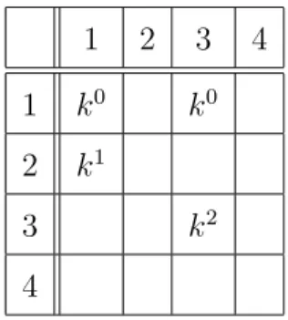
Example 5.1: Consider a 4-by-4 CBS, the corresponding Clos and the following traffic pattern:

C = {C0, C1, C2} C0 = {d011, d 0 13} C1 = {d121} C2 = {d233} Here, d0

Table 5.1: Traffic pattern for example 5.1 1 2 3 4 1 k0 k0 2 k1 3 k2 4

On CBS, there exists an optimal policy πCBS _{which transmits flows d}1 21 and

d2₃₃ in the first k time slots, d0₁₁ in the second k time slots and d0₁₃ in the third k time slots. In this case, CCTs become

t0(πCBS) = 3k

t1(πCBS) = k

t2(πCBS) = k

and the TCCT is calculated as;

T (πCBS) = 5k on CBS.

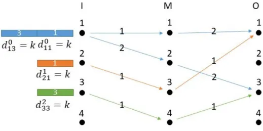
Figure 5-1: Traffic pattern C on a 4-by-4 Clos

On fig. 5-1, coflows are identified by different colors and the numbers on the flows denote their output ports. Arrows show how coflows separate and transmit their flows. The number on the arrow stands for the timing of the k time slots during which the separation or transmission happens in the direction of the arrow.

On Clos, coflow C0 can take advantage of the intermediate ports by

sep-arating its flows for the output ports 1 and 3 while waiting for coflows C1 and C2

to complete. This way, it will be able to transmit its packets to the output ports 1 and 3 in parallel when its turn comes. For this purpose, the optimal policy on Clos, πClos_{, first allocates the intermediate ports 1 and 2 for coflow C}

0, 3 for C1 and 4 for

C2. Then, during the first k time slots, it transmits flow d121 from the input port 2

to the output port 1 via the intermediate port 3 and flow d2

33 from the input port

3 to the output port 3 via the intermediate port 4. Hence, both coflows C1 and C2

complete in k time slots on Clos under πClos_{. Moreover, also during the first k time}

slots, it transmits flow d0₁₁ from the input port 1 to the intermediate port 1. This enables πClos _{to transmit the flows d}0

11 and d013 in parallel by using different

transmitted from the input port 1 to the output port 3 via the intermediate port 2. Hence, coflow C0 completes in 2k time slots on Clos under πClos. Finally, under πClos;

t0(πClos) = 2k t1(πClos) = k t2(πClos) = k Then, TCCT becomes; T (πClos) = 4k on Clos.

Finally, for this traffic pattern, improvement ratio becomes;

IR(C) = (5k − 4k)/5k = 1/5

whereas the coflow improvement ratio for coflow C0 under policies πCBS and πClos

becomes;

IR(C0) = (3k − 2k)/3k = 1/3

Notice that the key idea for achieving shorter TCCTs on Clos is ’separating’ flows that share the same input port but go to different output ports while their output ports are busy accepting other flows under the optimal policy. To facilitate the discussion of the following examples, we define dependent flows as exactly these flows that share the same origin yet have different destinations whereas independent flows are defined as flows having different origins if they have different destinations. We also denote coflows by letters in the subsequent examples to avoid any confusion of port and coflow indices as there will be many coflows and ports involved in these examples.

Once separation of dependent flows is identified as the key step in reducing TCCTs on Clos, it should be asked whether an algorithm should prioritize

separa-The examples 5.2 and 5.3 investigate this question in more detail and show that the answer depends on the characteristics of the traffic pattern considered:

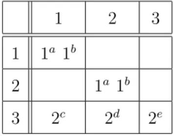
Example 5.2: Consider an N-by-N Clos (N ≥ 16) and the following traffic pattern: C = {Ca, Cb, Cc, Cd, Ce} Ca = {da11, d a 22} Cb = {db11, d b 22} Cc= {dc31} Cd= {dd32} Ce = {de33} Here, da

11, da22, db11 and db22 all have size 1 whereas dc31, dd32 and de33 have size 2. Table

5.2 gives a more visual representation of the traffic pattern:

Table 5.2: Traffic pattern for example 5.2

1 2 3

1 1a 1b

2 1a 1b

3 2c 2d 2e

Now, if the packets from coflow Ce are transmitted before packets in Cc and

Cd, then there exists a policy πClos under which;

tc(πClos) = 4

td(πClos) = 6

te(πClos) = 2

In this case, TCCT becomes;

T (πClos) = 1 + 2 + 4 + 6 + 2 = 15

Note that this policy achieves the minimum TCCT possible for this traffic pattern on Clos, thus, is an optimal policy. However, if coflows Cc and Cd are separated first,

before transmitting coflow Ce, then we obtain another, sub-optimal, policy πClosunder

which; ta(πClos) = 1 tb(πClos) = 2 tc(πClos) = 4 td(πClos) = 4 te(πClos) = 6

In this case, TCCT becomes;

T (πClos) = 1 + 2 + 4 + 4 + 2 = 17

Note that this policy achieves the minimum TCCT given the condition that Cc and

Cd are separated first. Consequently, in this example, transmitting coflow Ce first

minimizes TCCT, implying that for this traffic pattern, prioritizing transmission over separation yields the optimal policy on Clos.

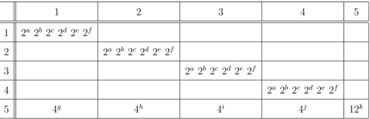
C = {Ca, Cb, Cc, Cd, Ce, Cf, Cg, Ch, Ci, Cj} Ca= {da11, d a 22, d a 33, d a 44} Cb = {db11, d b 22, d b 33, d b 44} Cc = {dc11, d c 22, d c 33, d c 44} Cd= {dd11, d d 22, d d 33, d d 44} Ce = {de11, d e 22, d e 33, d e 44} Cf = {df11, d f 22, d f 33, d f 44} Cg = {dg51} Ch = {dh52} Ci = {di53} Cj = {d j 54} Ck = {dk55} Here, da ii, dbii, dcii, ddii, deii, d f

ii, i ∈ {1, 2, 3, 4} all have size 2 whereas d g

51, dh52, di53 and d j 54

have size 4. dk

55 has size 12. Table 5.3 gives a more visual representation of the traffic

Table 5.3: Traffic pattern for example 5.3 1 2 3 4 5 1 2a 2b 2c 2d 2e 2f 2 2a ₂b ₂c ₂d ₂e ₂f 3 2a ₂b ₂c ₂d ₂e ₂f 4 2a ₂b ₂c ₂d ₂e ₂f 5 4g ₄h ₄i ₄j ₁₂k

To minimize TCCT, coflows at input ports 1, 2, 3 and 4 should be transmit-ted first. For the coflows in port 5, as in example 5.2, we will consider two strategies: • Coflow Ck is transmitted before coflows Cg, Ch, Ci and Cj. Then, there exists a

policy πClos under which;

ta(πClos) = 2 tb(πClos) = 4 tc(πClos) = 6 td(πClos) = 8 te(πClos) = 10 tf(πClos) = 12 tg(πClos) = 16 th(πClos) = 20 ti(πClos) = 24 tj(πClos) = 28

In this case, TCCT becomes;

T (π1) = 2 + 4 + 6 + 8 + 10 + 12 + 16 + 20 + 24 + 28 + 12 = 142

• Coflows Cg, Ch, Ci and Cj are separated before transmitting coflow Ck. Then

there exists a separating policy πClos _{under which;}

ta(πClos) = 2 tb(πClos) = 4 tc(πClos) = 6 td(πClos) = 8 te(πClos) = 10 tf(πClos) = 12 tg(πClos) = 16 th(πClos) = 16 ti(πClos) = 16 tj(πClos) = 16 tk(πClos) = 28

In this case, TCCT becomes;

T (πClos) = 2 + 4 + 6 + 8 + 10 + 12 + 16 + 16 + 16 + 16 + 28 = 134 Consequently, in this example, transmitting coflow Ckafter separating other

sep-given above is not the optimal one, the optimal policy also separates the coflows at the input port 5, showing that separation is indeed prioritized over transmission in the optimal case. (Optimal policy achieves a shorter TCCT by interleaving the flows in a complicated way.) Finally, as examples 5.2 and 5.3 show, the decision to separate or transmit flows at any given input port depends on the rest of the traffic pattern. Example 5.4 below generalizes this observation:

Example 5.4: Consider the traffic pattern where at an input port I there are m dependent coflows, Ci, i ∈ {1, ..., m} with sizes equal to a and another

depen-dent coflow C0 with size equal to d ≥ a. Assume that each of the Ci aims to transmit

to a different output port, i.e to m output ports in total and due to the traffic between these m output ports and other input ports, they cannot start transmitting before time n = (m−1)a ≥ d. On the other hand, we assume that C0 can transmit whenever

I is idle. Notice that this is a generalization of the situation in ports 3 and 5 in the examples 5.2 and 5.3 respectively. Similar to these examples, there are two options in favor of either transmission of C0 or separation of Ci:

• While Ci wait for their turn, node I can start transmitting C0 after which it

proceeds to transmit Ci. Under this policy;

t0(π) = d

ti(π) = n + ia

Hence, TCCT becomes;

T (π) = d+((n+a)+(n+2a)+(n+3a)+...+(n+ma)) = d+mn+m(m+1)a/2

• In the second option, node I can start separating Ci while they wait for their

before it can start its transmission. Hence, under this policy;

t0(π) = n + a + d

ti(π) = n + a

Hence, TCCT becomes;

T (π) = (n + a + d) + (n + a)m

Finally, the difference between TCCTs for the two cases, ∆, equals;

= [(n + a + d) + (n + a)m] − [d + mn + m(m + 1)a/2] = n + a + am/2 − am2/2

= 3am/2 − am2/2 = (3 − m)am/2

∆ is non-negative when m ≤ 3, implying that for such a node I with m = 2 or 3, transmitting C0 first minimizes the TCCT as in example 5.2. If m = 1, transmitting

is the best possible option under any traffic pattern as there is nothing to separate. On the other hand, separating Ci first before transmitting C0 becomes the optimal

course of action for minimizing TCCT when 4 ≤ m as in example 5.3.

Examples 5.2, 5.3 and 5.4 show that the decision to separate or transmit depends on the rest of the traffic pattern. For instance, when there are many mice flows occupying the output ports needed by elephant flows, it makes sense to separate these elephant flows while they wait for the smaller flows to complete. Hence, these elephant flows can later be transmitted in parallel. However, in general, it might be more reasonable to transmit flows whenever the opportunity arises rather than using available resources to separate flows that cannot be transmitted at that moment. Although the optimal decision depends on the specifics of the traffic pattern, it is

many flows with similar sizes.

Another key question to ask is whether the optimal policy on Clos preserves the transmission or completion order of the flows given by the optimal policy on CBS. Traffic patterns above which shed light on the question of separation vs. transmission can be used to answer this question as well:

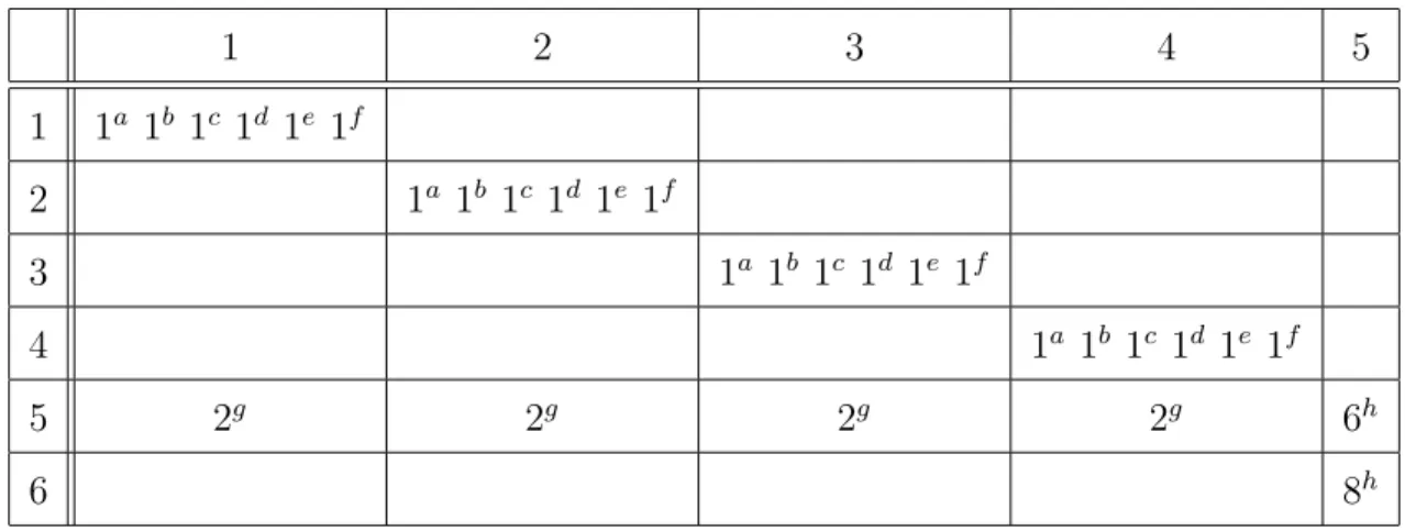
Example 5.5: Consider an N-by-N CBS (N ≥ 16), the corresponding Clos and the following traffic pattern:

C = {Ca, Cb, Cc, Cd, Ce, Cf, Cg, Ch} Ca= {da11, d a 22, d a 33, d a 44} Cb = {db11, d b 22, d b 33, d b 44} Cc = {dc11, d c 22, d c 33, d c 44} Cd= {dd11, d d 22, d d 33, d d 44} Ce = {de11, d e 22, d e 33, d e 44} Cf = {df11, d f 22, d f 33, d f 44} Cg = {dg51, d g 52, d g 53, d g 54} Ch = {dh55, d h 65}

Here, da_ii, db_ii, dc_ii, dd_ii, de_ii, df_ii, i ∈ {1, 2, 3, 4} all have size 1 whereas dg₅₁, dg₅₂, dg₅₃ and dg₅₄ have size 2. dh

55 and dh65 have sizes 6 and 8 respectively. Table 5.4 gives a

Table 5.4: Traffic pattern for example 5.5 1 2 3 4 5 1 1a 1b 1c 1d 1e 1f 2 1a ₁b ₁c ₁d ₁e ₁f 3 1a ₁b ₁c ₁d ₁e ₁f 4 1a ₁b ₁c ₁d ₁e ₁f 5 2g ₂g ₂g ₂g ₆h 6 8h

To minimize the TCCT, coflows Ca, Cb, Cc, Cd, Ce and Cf should be

trans-mitted first before any other coflow. However, the order of transmission for the coflows Cg and Ch on the input port 5 depends on the topology of the network.

• On CBS, the optimal policy requires coflow Ch to have priority over coflow Cg

on the input port 5. Under this policy πCBS_;

ta(πCBS) = 1 tb(πCBS) = 2 tc(πCBS) = 3 td(πCBS) = 4 te(πCBS) = 5 tf(πCBS) = 6 tg(πCBS) = 14 th(πCBS) = 14

In this case, TCCT becomes;

T (πCBS) = 1 + 2 + 3 + 4 + 5 + 6 + 14 + 14 = 49

Note that coflow Cg cannot have priority of transmission in this case because

its output ports are blocked for the first 6 time slots.

• On Clos, the optimal policy requires coflow Cg to separate its flows while waiting

for its output ports to be free. Then, under this optimal policy πClos; ta(πClos) = 1 tb(πClos) = 2 tc(πClos) = 3 td(πClos) = 4 te(πClos) = 5 tf(πClos) = 6 tg(πClos) = 8 th(πClos) = 14

In this case, TCCT becomes;

T (πClos) = 1 + 2 + 3 + 4 + 5 + 6 + 8 + 14 = 43

Note that if coflow Ch had priority on port 5 as in the previous case, then,

coflow Cg would not be able to use the separation advantage of the Clos and

the TCCT would have been 49 again instead of 43.

different on Clos and CBS. This further implies that the completion order of coflows can also be different under optimal policies on Clos and CBS. A slight change on the traffic pattern above, i.e making dg₅₁= 3 gives such an example.

Finally, we can summarize the insights obtained through these examples in the following points:

• Clos can achieve lower minimum TCCTs than CBS for some traffic patterns through separation of dependent flows.

• At any input port, the decision to separate or transmit dependent flows depends on the rest of the traffic pattern under the optimal policy.

• Coflow transmission orders at any given input port as well as the order of CCTs can be different on Clos and CBS under optimal policies.

Chapter 6

Bounds on the Maximum

Improvement Ratio

This section aims to establish bounds on the maximum improvement ratio of traffic patterns and the maximum coflow improvement ratio under order preserving optimal policies.

Before moving onto the examples and theorems, it is useful to reiterate some of the terms that will be heavily used in the subsequent sections:

• C and Ckstand for a traffic pattern and the kthcoflow within that traffic pattern

respectively. • dk

ij stands for the flow within coflow Ck with the input port i and the output

port j.

• dk _{is defined as the total size of coflow C} k:

dk= X

i∈I,j∈O

dk_ij

• tk(π) denotes the completion time of coflow Ck under policy π.

times under the optimal policies. Hence, for any Ck−1 and Ck under policy π;

tk−1(π) ≤ tk(π)

• N denotes for the number of input (as well as output and intermediate) ports in CBS and Clos.

6.1

Lower Bound on the Maximum Improvement

Ratios

This section demonstrates that for any number smaller than 1/e, it is possible to find a traffic pattern with an improvement ratio larger than that number. It also shows that for any coflow improvement ratio smaller than 1/2, it is possible to find a coflow surpassing this ratio under order preserving optimal policies.

To prove the 1/e lower bound for the maximum improvement ratio, we should investigate the features of traffic patterns that have the strongest impact on their improvement ratios. We know that Clos achieves smaller TCCTs by separating coflows while they wait for other coflows to complete under the optimal policy. Hence, to maximize the improvement ratio, we should construct a traffic pattern in which dependent flows within each coflow will be totally separated by the time their turn comes under the optimal policy so that they can be transmitted in parallel. To demonstrate this idea, let’s consider a traffic pattern on Clos in which each coflow consists of two equally sized flows sharing an input port and going to two different output ports. In this traffic pattern, every coflow will have the same two output ports 1 and 2 as the destination for their flows. Fig. 6-1 below shows a part of this traffic pattern.

Figure 6-1: Traffic pattern on an N-by-N Clos

On fig. 6-1, coflows are identified by different colors and arrows show how coflows separate one of their flows by sending them to the pointed intermediate ports while waiting for their turn under the optimal policy. The common output ports 1 and 2 are circled by a red box.

Now, take coflow Ck of size dk within this traffic pattern C. Ck has two

equally sized flows with dk/2 packets sharing an input port and going to two different output ports. For Ck to totally separate its flows on Clos, it should be waiting for

at least dk/2 time slots under the given policy so that it has enough time to move one of its two flows to an intermediate port. On the other hand, Ck can wait at most

tk−1(πClos) time slots on Clos under the optimal policy πClos; because coflows that

πClos_{. Hence,}

tk−1(πClos) ≥ dk/2

Since πClos _{should also achieve the minimum possible CCT for each coflow without}

increasing the CCTs of other coflows, we can take

tk−1(πClos) = dk/2 (∗)

Finally, once its flows are separated, Ck can transmit all of its flows in dk/2 time slots

in parallel, implying that

tk(πClos) = tk−1(πClos) + dk/2 = dk

Combining this with the observation

tk(πClos) = dk+1/2

for coflow Ck+1, achieved by replacing k with k + 1 in equation (∗) above, we obtain

dk+1 = 2dk

The result above demonstrates that the traffic patterns whose flows can be totally parallelized on Clos under the optimal policy should consist of exponentially sized coflows. Since we assumed that flows had their packets destined to two output ports, the exponent becomes 2 in this case. The following example embodies this idea by considering a similar traffic pattern C on 10-by-10 CBS and Clos:

Example 6.1

C1 = {d131, d 1 32} C2 = {d241, d 2 42} C3 = {d351, d 3 52} C4 = {d461, d 4 62}

Sizes of these flows are given below:

d0₁₁ = d0₂₂= d1₃₁= d1₃₂= 1 d2₄₁= d2₄₂= 2 d3₅₁= d3₅₂= 4 d4₆₁= d4₆₂= 8 Then, the total coflow sizes become:

d0 = d1 = 2 d2 = 4 d3 = 8 d4 = 16

Fig. 6-2 below shows C on a 10-by-10 Clos. Coflows are identified by differ-ent colors and the numbers on the flows denote their output ports:

Figure 6-2: Traffic pattern C on a 10-by-10 Clos

On fig. 6-2, coflows are identified by different colors and the numbers on the flows denote their output ports. Arrows show how coflows separate their flows by sending them to the pointed intermediate ports while waiting for their turn under the optimal policy. The common output ports 1 and 2 are circled by a red box.

Under the optimal policy πCBS _{on CBS, smaller coflows will be prioritized}

over larger ones to achieve the minimum TCCT. Hence, coflow C0 will be transmitted

first, followed by the coflows C1, C2, C3 and C4. Note that since all of the coflows have

output ports 1 and 2 as their destinations, whenever a coflow finishes transmission of its flows for one of these output ports, the next coflow starts transmitting to this output port.

πCBS _{first transmits flows d}0

11 and d022 in C0 to the output ports 1 and 2,

thus, completing C0 in the first time slot.

During the second time slot, it transmits flow d1

31from C1 to the output port

the output port 1. Hence, C1 is completed in 3 time slots.

In a similar pattern, within the next 2 time slots, πCBS _{transmits the}

re-maining two packets in the flows d2

41 and d242 within C2 while both flows d131 and d132

in coflow C3 send one packet to each of the output ports 1 and 2. In this case, C2

completes in 5 time slots.

Finally, by the 5th _{time slot, coflows C}

0, C1 and C2 are totally transmitted,

thus, enabling πCBS to transmit the coflows C3 and C4 in parallel. Hence, the

re-maining 6 packets within C3 are sent by the 5 + 6 = 11th time slot. Since C4 has size

16, we find that it is completed by the 5 + 16 = 21st time slot via a similar analysis. Given this optimal policy, we obtain the following CCTs:

t0(πCBS) = 1

t1(πCBS) = 3

t2(πCBS) = 5

t3(πCBS) = 11

t4(πCBS) = 21

and the TCCT becomes;

TCBS = T (πCBS) = 41

Notice that under πCBS_{, CCTs follow a specific pattern:}

t0(πCBS) = 1

t1(πCBS) = d1+ d0 = 3

t2(πCBS) = d2+ d0 = 5

t3(πCBS) = d3+ d1+ d0 = 11

t4(πCBS) = d4+ d2+ d0 = 21

to transmit. Under πClos_{, the intermediate ports 1 to 10 are allocated to the flows}

d0

11, d022, d131, d132, d241, d242, d351, d352, d461 and d462 respectively.

πClos _{begins by first transmitting d}0

11 and d022 within coflow C0 to the output

ports 1 and 2 via the intermediate ports 1 and 2. Hence, C0 is completed in one time

slot. Meanwhile, coflows C1, C2, C3 and C4 send one packet from the flows d132, d242,

d3

52 and d462 to the intermediate ports 4, 6, 8 and 10 respectively.

Notice that by the 2nd time slot, coflow C1 is completely separated, thus,

enabling πClos _{to transmit the flows d}1

31at the input port 3 and d132at the intermediate

port 4 to the output ports 1 and 2 in parallel. To reach output port 1, d1₃₁ uses the intermediate port 3 which was allocated for it by πClos_{. Hence, C}

1 is completed in

two time slots. Meanwhile, coflows C2, C3 and C4 send one more packet from the

flows d2

42, d352 and d462 to the intermediate ports 6, 8 and 10.

Similar to the step above, by the 3rd time slot, coflow C2 is completely

separated, thus, enabling πClos _{to transmit the flows d}2

41 at the input port 4 and d242

at the intermediate port 6 to the output ports 1 and 2 in parallel. Since both flows include two packets, C2 is completed in 2 + 2 = 4 time slots. To access output port 1,

d2₄₁ uses the intermediate port 5 allocated to it. Meanwhile, coflows C3 and C4 send

two more packet from the flows d3

52 and d462 to the intermediate ports 8 and 10.

The pattern above repeats itself for the coflows C3 and C4. This way, C3

sends all of d3

52 to the intermediate port 8 while C4 sends d462 to the intermediate port

10. Intermediate ports 7 and 9 are then used for the transmission of d3₅₁ and d4₆₁ to the output port 1. By a similar analysis, we find that C3 and C4 are completed in 8

Given this optimal policy, we obtain the following CCTs: t0(πClos) = 1 t1(πClos) = 2 t2(πClos) = 4 t3(πClos) = 8 t4(πClos) = 16

and the TCCT becomes;

TClos= T (πClos) = 31

Notice that under this optimal policy on Clos, CCTs again follow a specific pattern: t0(πClos) = 1 t1(πClos) = d1 = 2 t2(πClos) = d2 = 4 t3(πClos) = d3 = 8 t4(πClos) = d4 = 16

Finally, for this traffic pattern, the improvement ratio becomes;

IR(C) = 41 − 31

41 =

10

41 ≈ 0.25

Although example 2 consisted of five coflows each of which had two flows going to two output ports, it is possible to generalize this example in two ways. First, we can increase the number of coflows in C, and subsequently, sizes of the topologies CBS and Clos. Second, we can have coflows consisting of more flows going to more than two destination ports. The following paragraph constructs a general traffic pattern CS,B in which there are SB + 1 coflows and each coflow consists of B equally

sized flows with B different destination ports. Note that the +1 within SB + 1 denotes coflow C0. Given this notation, a more accurate name for the traffic pattern

in example 2 would be C2,2.

CS,B = {Ck|k ∈ {0, ..., SB}}

C0 = {d0ii|i ∈ {1, ..., B}}

d0_ii= D ∀i ∈ {1, ..., B}

Here, D is chosen as the minimum integer such that D(BSB−1/(B − 1)SB) is an integer. Hence, when B = 2 as in example 2, D can be chosen as 1. In fact, D can be chosen as any integer such that the flows consist of integer number of packets.

Ck = {dkk+B,j|j ∈ {1, ..., B}} ∀k ∈ {1, ..., SB}

dk_k+B,j = DB

k−1

(B − 1)k ∀k ∈ {1, ..., SB} ∀j ∈ {1, ..., B}

Notice that each coflow Ck, k ∈ {1, ..., SB} consists of B equally sized flows sharing

the same input port k + B. Hence,

d0 = DB dk = D( B

B − 1)

k _{∀k ∈ {1, ..., SB}}

As in the example 2, coflow sizes follow an exponential pattern. For instance, having the number of output ports equal to B = 2 gives a factor of B/(B − 1) = 2.

Finally, for the sake of simplicity, define this factor as

β = B

B − 1 which gives

For the general example, we assume Clos to have adequate number of inter-mediate ports to separate all of the flows in each coflow and transmit them in parallel. Consequently, N can be taken as B + SB2_.

Finally, having specified the traffic patterns CS,B, we can calculate the

min-imum TCCTs TCBS and TClos on N-by-N, N = B + SB2_{, CBS and Clos for these}

patterns:

For TCBS to obtain its minimum value, smaller coflows should be transmit-ted before larger coflows as in example 2. Since all of the coflows share the same B destination ports, coflow CBs+j cannot start its transmission before πCBS transmits

the coflows C0 and CBi+j, ∀i ∈ {1, ..., s − 1}, to their destination ports. This

ob-servation implies a strict ordering for CCTs under which, similar to the pattern in example 2 for CCTs on CBS, we obtain;

tBs+j = d0+ s

X

k=0

dBk+j j ∈ {1, ..., B}, s ∈ {0, ..., S − 1} Then, TCBS is calculated as;

SB X k=0 tk = d0+ S−1 X i=0 B X j=1 tBi+j = (SB + 1)d0+ S−1 X i=0 B X j=1 i X k=0 dBk+j = (SB + 1)D + S−1 X i=0 B X j=1 i X k=0 D( B B − 1) Bk+j = D[B( β B βB_{− 1})β BS ] − o(βBS)

On the other hand, for TClos _{to achieve its minimum value, coflows should}

separate their flows going to different output ports while waiting for previous coflows to complete under πClos_{. For this purpose, π}Clos _{allocates B intermediate ports,}

kB + 1, ..., kB + B, for each coflow Ck. Among these ports, kB + 2, ..., kB + B receive

the flows dk

k+B,2, ..., dkk+B,B respectively during the separation phase until the output

ports become free for Ck to be transmitted. The intermediate port kB + 1, however,

remains idle for the flow dk

k+B,1 which will later be transmitted to the output port 1

simultaneously with the other separated flows. Hence, when its turn comes, Ck will

be able to transmit all of its packets at these intermediate ports and the input port in parallel. For instance, in example 2 where B = 2, coflows C1, C2, C3 and C4 send half

of their packets, i.e those going to the output port 2 to the intermediate ports 4, 6, 8 and 10 respectively. Then, the intermediate ports 3, 5, 7 and 9 are used to transmit the remaining half of the packets, i.e those going to the output port 1, simultaneously with those moved to the intermediate ports.

Using the policy above, we find that under πClos_{, CCT for each coflow equals}

the total size of the coflow as shown in example 2. Notice that the CCT for a coflow Ck cannot be smaller than dk in this traffic pattern as the flows within each coflow

share the same input port. Hence, total separation yields the minimum possible CCT on Clos for this traffic pattern. Consequently, TClos is calculated as;

SB X k=0 dk = SB X k=0 Dβk = Dβ SB+1_{− 1} β − 1 = D[BβSB] − o(βSB)

In this case, the improvement ratio for CS,B becomes;

IR(CS,B) = TCBS− TClos TCBS = 1 βB − o(βSB) βSB

Placing the value of β, we can obtain the improvement ratio in terms of B: IR(CS,B) = (1 − 1 B) B₋ o(β SB₎ βSB

In the context of example 2 where B = 2 and S = 2, (1 − (1/B))B _term

equals 1/4 and the o(βSB)/βSB term equals approximately 0.0061. Finally, this ex-pression for the improvement ratio enables us to state the following theorem:

Theorem 6.1: There exists a set of traffic patterns, Γ∗ such that supC∈Γ∗ IR(C) = 1/e

Proof of Theorem 6.1: Consider the set of traffic patterns

Γ∗ = {CS,B|B ∈ {2, ...}, S ∈ {2, ...}}

where CS,B is defined above. As o(βSB)/βSB goes to zero with increasing S and

(1 − 1/B)B _{approaches 1/e from below with increasing B;}

limB→∞ limS→∞ IR(CS,B) =

1 e = IR where the improvement ratio approaches the limit from below.

Hence, we can conclude that for any traffic pattern C ∈ Γ∗, IR(C) < 1/e and for any r < 1/e, there exists a traffic pattern Cr ∈ Γ∗ and topologies Clos and

CBS such that IR(Cr) > r. This concludes the proof.

The traffic patterns found above can also be used to find a lower bound for the maximum coflow improvement ratio under order preserving optimal policies. First, notice that the policies used to schedule these traffic patterns are not only optimal but also order preserving in the sense that the order of CCTs is the same on CBS and Clos. Second, consider the coflow C within the traffic pattern C

where 2 ≤ S. Now, the completion time for CBs+j is equal to tBs+j(πCBS) = d0+ s X k=0 dBk+j = D + s X k=0 D( B B − 1) Bk+j = D[1 + βj(β B(s+1)_{− 1} βB_{− 1} )]

on CBS under order preserving optimal policies.

On the other hand, its completion time equals tBs+j(πClos)

= dBs+j = D[βBs+j]

on Clos under the same set of policies. Consequently, the coflow improvement ratio for CBs+j becomes IR(CBs+j) = tBs+j(π CBS_{) − t} Bs+j(πClos) tBs+j(πCBS) = D[1 + β j_((βB(s+1)_{− 1)/(β}B_{− 1))] − D[β}Bs+j_] D[1 + βj_((βB(s+1)_{− 1)/(β}B_{− 1))]} = β Bs+j_{+ β}B_{− β}j_{− 1} βB(s+1)+j_{+ β}B_{− β}j_{− 1}

Finally, using this expression for IR(CBs+j), we can state the following

the-orem:

Theorem 6.2:

supCk∈C∈Γ∗ IR(Ck) = 1/2

above increases as j decreases, thus, to obtain the maximum coflow improvement ratio for the coflows within CS,B, we should set j to be 1. Moreover, the ratio approaches

1/βB _{from above as s increases, implying that s should also be set to its lowest value,}

i.e 0, for the same purposes. Then the ratio becomes

IR(C1) = β B_{− 1} βB+1_{+ β}B_{− β − 1} = 1 β + 1 = B − 1 2B − 1 and; limB→∞ IR(C1) = 1 2

where the coflow improvement ratio for C1 approaches the limit from below.

Finally, under order preserving optimal policies, the maximum coflow im-provement ratio for the coflows in any CS,B ∈ Γ∗ is achieved for the coflow C1 and

IR(C1) < 1/2 for any number of output ports B. Moreover, for any r < 1/2, it

is possible to find a number Br and construct the corresponding coflow C1 and the

traffic pattern CS,Br ∈ Γ

∗ _{such that IR(C}

1) > r. This concludes the proof.

6.2

Upper Bound on the Maximum Improvement

Ratios

This section shows that the coflow improvement ratio for any coflow within any traffic pattern C ∈ Γs has to be smaller than 1/2 under order preserving optimal policies.

(Γs was defined as the set of traffic patterns for which there exist order preserving

optimal policies on CBS and Clos.) Similarly, it establishes 1/e as an upper bound for the improvement ratios of all traffic patterns. Before proving these results, it is imperative to define the following notation which will be used throughout this section.

Under a given policy π and in a specific coflow Ck; for the collection Sp with

size d (Sp was defined as the last collection within Ck to send a packet on CBS);

• Define dCBS,I _{as the number of time slots during which one of the input ports}

on CBS transmits a packet belonging to Sp.

• Similarly, define dCBS,O _{as the number of time slots during which one of the}

output ports on CBS receives a packet belonging to Sp.

• dClos,I _{and d}Clos,O _{are defined similarly on Clos.}

• Define

wCBS := tCBS_p − dCBS,O

and,

wClos:= tClos_p − dClos,O

• Let B denote the maximum number of output ports that any coflow or collection in C sends packets.

The following lemma regarding these definitions will play an important role in the subsequent proofs:

Lemma 6.0:

dCBS,I = dCBS,O = dClos,I = d d/B ≤ dClos,O ≤ d

Proof of Lemma 6.0: First, notice that all the flows within a collection share the same input port which should be active for exactly d time slots to be able to send all of the packets within Sp. Hence,

during the same time slot. Hence, on CBS, the number of time slots during which one of the output ports receives a packet belonging to Sp should be equal to the

number of time slots during which the input port of Sp transmits a packet belonging

to Sp. Hence,

dCBS,O = dCBS,I = d

On the other hand, an output port on Clos can receive at most d packets belonging to the flows within Sp, implying that

dClos,O ≤ d

However, in the best case, Sp consists of B equally sized flows going to the B output

ports, which can be separated and transmitted in parallel to their destinations. Then, the B output ports will be simultaneously busy with receiving the packets in Sp, thus

receiving all of the packets in Sp during d/B time slots. Consequently,

d/B ≤ dClos,O

Theorem 6.3: IR(Ck) ≤ 1/2 ∀Ck ∈ C ∈ Γs under order preserving

opti-mal policies.

Proof of theorem 6.3 depends on the following lemmas. Note than 2 ≤ B in all of these proofs because otherwise, Clos cannot achieve a smaller latency than CBS for any coflow.

Lemma 6.1: For any Ck ∈ C ∈ Γs, if assumption 1 holds for Sp ∈ Ck and

if (B − 1)d/B ≤ wClos_{, then w}CBS _{≤ Bw}Clos _{under order preserving optimal policies.}

(Reminder that under assumption 1, Sp sends the last packet of Ck on both CBS

any packet from a coflow completing after Ckduring any of the wCBStime slots as this

would violate the optimality of the order preserving policies. Hence, during the wCBS

time slots, packets in Sp should be waiting on packets from collections completing

before Sp. Now, to obtain the maximum possible value for wCBS with respect to

wClos_{, make the following assumption: All of the packets other than those of S} p,

transmitted during the dClos,O _{time slots on Clos, belong to collections completing}

before Sp and all of these packets are transmitted during the wCBS time slots on CBS

rather than dCBS,O_.

Second, we observe that for the packets from previous collections to block packets of Sp, they should be transmitted to Sp’s output ports on CBS. Since there

are at most B such output ports, there can at most be (B − 1)dClos,O such packets introduced to wCBS _{from d}Clos,O_{. Transmission of S}

p is delayed as long as all of the B

output ports receive a packet from previous collections, i.e as long as the least number of introduced packets received by any of the B output ports. This least number is at most equal to the total number of packets divided by B, i.e its maximum value has to be (B − 1)dClos,O_{/B. Consequently, introduction of the extra packets from d}Clos,O

time slots can halt the transmission of packets from Sp for at most (B − 1)dClos,O/B

extra time slots on CBS. (It can potentially be lower due to the interleaving, on CBS, of packets originally transmitted within wClos and dClos,O time slots on Clos.) Finally, from the observations above, wCBS _{can at most be w}Clos _{plus the}

maximum delay due to the packets introduced to wCBS, i.e (B − 1)dClos,O/B: wCBS ≤ wClos_{+ (B − 1)d}Clos,O_/B

As (B − 1)d/B ≤ wClos _{and d}Clos,O _{≤ d;}

wCBS ≤ wClos_{+ (B − 1)d}Clos,O_{/B ≤ w}Clos_{+ (B − 1)d/B ≤ 2w}Clos_{≤ Bw}Clos

Proof of Lemma 6.2: Proof by cases. First, notice that d ≤ tClos p =

wClos_{+ d}Clos,O _{as d = d}Clos,I _{and d}Clos,I _{≤ t}Clos

p . Now, we can focus on the following

cases:

• Case 1: If wClos _{≥ (B − 1)d/B, then d}Clos,O _{can be as small as d/B.}

Con-squently, IR(Sp) (6.1) = (w CBS_{− w}Clos_{) + (d − d}Clos,O₎ wCBS_{+ d} (6.2) ≤ d − d Clos,O wClos_{+ d} (6.3) ≤ d − (d/B) wClos_{+ d} (6.4) ≤ d − (d/B) (B − 1)d/B + d (6.5) = B − 1 2B − 1 (6.6)

Here, 6.2 follows from the definition of IR(Sp) whereas 6.4 and 6.5 follow from

the assumption on wClos _{and the observation on d}Clos,O _{given above. 6.3 is a}

simple inequality due to the fact that wCBS ≤ wClos_.

• Case 2: If wClos _{≤ (B − 1)d/B, then d − w}Clos _{≤ d}Clos,O_{. Consequently,}

IR(Sp) (6.7) = (w CBS_{− w}Clos_{) + (d − d}Clos,O₎ wCBS_{+ d} (6.8) ≤ d − d Clos,O wClos_{+ d} (6.9) ≤ w Clos wClos_{+ d} (6.10) ≤ (B − 1)d/B (B − 1)d/B + d (6.11) = B − 1 (6.12)

Here, 6.9 and 6.10 follow from the assumption on wClos _{and the observation on}

dClos,O_{. 6.8 is a simple inequality due to the fact that w}CBS _{≤ w}Clos_.

Finally, IR(Sp) ≤ (B − 1)/(2B − 1) ≤ 1/2 when wCBS ≤ wClos. Note that

the bound becomes tight when wClos_{= (B − 1)d/B, d}Clos,O _{= d/B and as B goes to}

infinity.

Corollary 6.1: Assume that wCBS _{≤ w}Clos_{. Given d and B as constants,}

when IR(Sp) attains its maximum value under order preserving (but not necessarily

optimal) policies, wClos _{= (B − 1)d/B and d}Clos,O _{= d/B for S} p.

Lemma 6.3: If the assumption 1 holds for Sp and wClos ≤ wCBS, IR(Sp) ≤

1/2 under order preserving optimal policies.

Proof of Lemma 6.3: From lemma 6.1, we know that if (B−1)d/B ≤ wClos

and if the assumption 1 holds for Sp, then, wCBS ≤ BwClos under order preserving

optimal policies. Now, assume that wCBS _{= bw}Clos_{. Since IR(S}

p) can be expressed

as a function of dClos,O_{, w}Clos _{and b, we can find an upper bound for it by maximizing}

IR(Sp) with respect to dClos,O, wClos and b respectively. For this purpose, consider

the following two cases under a constant b:

• Case 1: If (B − 1)d/B ≤ wClos_{, then 1 ≤ b ≤ B and d}Clos,O _{can be as small as}

d/B. Hence; IR(Sp) (6.13) = (b − 1)w Clos_{+ (d − d}Clos,O₎ bwClos_{+ d} (6.14) ≤ (b − 1)w Clos_{+ (d − (d/B))} bwClos_{+ d} (6.15)

• Case 2: If wClos _{≤ (B − 1)d/B, then d − w}Clos _{≤ d}Clos,O_{. Hence;} IR(Sp) (6.16) = (b − 1)w Clos_{+ (d − d}Clos,O₎ bwClos_{+ d} (6.17) ≤ bw Clos bwClos_{+ d} (6.18)

As wClos ≤ (B − 1)d/B for this case, 6.18 attains its largest value when wClos

is at its largest, i.e when wClos _{= (B − 1)d/B.}

As the calculations above indicate, under both cases, the upper bounds for IR(Sp), i.e the expressions 6.15 and 6.18, reach their maximum values when

dClos,O _{= d/B and w}Clos _{= (B − 1)d/B regardless of the value of b. Moreover, placing}

dClos,O = d/B and wClos = (B − 1)d/B makes these upper bounds tight and equal as functions of b. Hence, to find the maximum value of IR(Sp) for a given d and B, we

should maximize the bound above with respect to b under the given constraints on wClos _{and d}Clos,O_{. Since the bound becomes}

bwClos

bwClos_{+ d} =

wCBS

wCBS_{+ d}

under these constraints, maximizing it with respect to b is equivalent to finding the maximum value of wCBS subject to the constraints on wClos and dClos,O:

When wClos _{= (B − 1)d/B and d}Clos,O _{= d/B, i.e when the coflow is totally}

separated on Clos, collections completing before Sp should send all of their packets

during the first wClos _{= (B − 1)d/B time slots. However, on CBS, packets from S} p

and the collections completing before Sp can be transmitted simultaneously to the B

output ports, implying that the previous collections do not have to send all of their packets during the wCBS time slots. Moreover, collections completing after Spon Clos

cannot send a packet to the B output ports before Sp on CBS because, in this case,

it would be possible to complete Sp, thus, Ck at an earlier time slot, contradicting the

slots. This implies that wCBS _{cannot be larger than w}Clos _{under order preserving}

optimal policies when wClos _{= (B − 1)d/B and d}Clos,O _{= d/B. As a result;}

IR(Sp) ≤ w CBS wCBS _{+ d} ≤ w Clos wClos_{+ d} = (B − 1)d/B (B − 1)d/B + d = B − 1 2B − 1 ≤ 1 2

We conclude by pointing out that the bound becomes tight for IR(Sp) as B increases.

Corollary 6.2: Assume that wClos≤ wCBS_{. Let π}Clos_{be the optimal policy}

for the traffic pattern C on Clos. Now, construct the (not necessarily optimal) policy πCBS such that

• The order of completion times for coflows is preserved.

• Sp is still the last collection to complete within Ck, thus, assumption 1 holds.

• πCBS _{minimizes TCCT on CBS given the above constraints on the order of}

completion times.

. Given d and B as constants, when IR(Sp) attains its maximum value under policies

πCBS _{and π}Clos_{, w}Clos_{= (B − 1)d/B and d}Clos,O _{= d/B for S} p.

Lemma 6.4: IR(Sp) ≥ IR(Ck) under order preserving optimal policies.

IR(Sp) = 1 − tClos p tCBS p Since

maxi∈I{tClosi }

maxi∈I{tCBSi } = maxi∈I{t Clos i } tCBS p ≥ t Clos p tCBS p ;

1 − IR(Ck) ≥ 1 − IR(Sp), implying that

IR(Sp) ≥ IR(Ck)

. Equality happens if and only if the last collection to complete on Clos and CBS is the same Sp, i.e, under assumption 1.

Lemma 6.5: If assumption 1 holds, IR(Sp) ≤ 1/2 under order preserving

optimal policies.

Proof of Lemma 6.5: From lemmas 6.2 and 6.3, we know that if as-sumption 1 holds, then IR(Sp) ≤ 1/2 under order preserving optimal policies for

both cases wClos ≤ wCBS _{and w}Clos _{≥ w}CBS_{. Consequently, if assumption 1 holds,}

then 1/2 has to be an upper bound for IR(Sp) under order preserving optimal policies.

Proof of Theorem 6.3: Proof by cases.

• Case 1: If IR(Ck) = IR(Sp), then the upper bound for IR(Ck) and IR(Sp)

has to be the same under order preserving optimal policies, which is 1/2 by lemma 6.5.