Une Approche Hybride de Simulation-Optimisation Basée sur la fouille de Données pour les problèmes d'ordonnancement

HAL Id: tel-00647353

https://tel.archives-ouvertes.fr/tel-00647353

HAL is a multi-disciplinary open access archive for the deposit and dissemination of sci-entific research documents, whether they are pub-lished or not. The documents may come from teaching and research institutions in France or abroad, or from public or private research centers.

L’archive ouverte pluridisciplinaire HAL, est destinée au dépôt et à la diffusion de documents scientifiques de niveau recherche, publiés ou non, émanant des établissements d’enseignement et de recherche français ou étrangers, des laboratoires publics ou privés.

Basée sur la fouille de Données pour les problèmes

d’ordonnancement

Atif Shahzad

To cite this version:

Atif Shahzad. Une Approche Hybride de Simulation-Optimisation Basée sur la fouille de Données pour les problèmes d’ordonnancement. Automatique / Robotique. Université de Nantes, 2011. Français. �tel-00647353�

UNIVERSITÉ DE NANTES

École polytechnique de l’Université de Nantes

_____

ÉCOLE DOCTORALE

« SCIENCES ET TECHNOLOGIE DE L’INFORMATION ET MATHEMATIQUES »

Année 2011

Une Approche Hybride de Simulation-Optimisation

Basée sur la Fouille de Données pour les Problèmes

d’ordonnancement

___________

THÈSE DE DOCTORAT

Discipline : Génie Informatique

Spécialité : Automatique et Génie Informatique

Présentée

et soutenue publiquement par

Muhammad Atif SHAHZAD

Le 17 fév. 2011, devant le jury ci-dessous

Rapporteurs Examinateurs

Henri PIERREVAL Professeur, IFMA, Clermont-Ferrand, France Jean-Charles BILLAUT Professeur, Université de Tours, France

Abdelhakim ARTIBA Professeur, Université de Valenciennes, France Christos DIMOPOULOS Asst. Professor, Nicosia, Cyprus

Directeur de thèse : Pierre CASTAGNA Professeur, Université de Nantes, France

Conencadrant : Nasser MEBARKI Maître de Conférences, Université de Nantes, France ED : 503-119 (Uniquement pour STIM et SPIGA)

1

Acknowledgment

This dissertation would not have been possible without the guidance and the help of several individuals who in one way or the other contributed and extended their valuable assistance in the preparation and completion of this work.

I would like to thank Professor Henri PIERREVAL and Professor Jean-Charles BILLAUT for accepting my request to examine this thesis as the official referees. I am also thankful to Professor Abdelhakem ARTIBA and Associate Professor Christos DIMOPOULOS for accepting the invitation to attend my thesis defense. I highly appreciate them all for sparing some time and being flexible in the dates despite their busy schedules.

My utmost gratitude to my advisor Professor Pierre CASTAGNA, for his steadfast en-couragement, kind concern and consideration during this work.

I would like to express the deepest appreciation to my thesis co-advisor, Dr. Nasser MEBARKI who continually and convincingly conveyed a spirit of research. His wide knowledge and logical way of thinking has been a great value for me. He provided me with an untiring help, valuables suggestions and detailed and constructive insightful comments throughout this work. Thank you very much for patiently correcting and edi-ting my manuscript as well. Without his guidance and persistent help this dissertation would have not been possible.

I greatly admire the persistent and meticulous attitude of Professor Jean-Jacque Loiseau, incharge of the research team ACSED (Analyse et Commande des Syst`emes `a Ev´enen-ments Discrets). I wish to extend my warmest thanks to all members of the team for their support and encouragement. In particular, I would like to thank Dr. Guillaume Pinot and Dr. Olivier Boutin for offering their advice and suggestions whenever I needed them. I would like to thank all the staff members at the IRCCyN for all their help, technical and moral support.

Special thanks goes to Mme Somia ASHRAF, who encouraged me a lot to initiate this work in France. Furthermore, I am greatly thankful to Miss Qudsia and Miss Brigette at Alliance Fran¸caise, Islamabad.

Where would I be without my family? My deepest gratitude goes to my family for their unflagging love and support throughout my life; this dissertation is simply impossible without them. I am greatly indebted to my father for his great care and attention, sparing no effort to provide the best possible environment for me to grow up and showing me the joy of intellectual pursuit ever since I was a child. Although he is no longer with us, he is forever remembered. I have no suitable words to describe the everlasting love of my mother. Her continuous support and unconditional love has been my greatest strength. Despite all the hardships in the life, she provided with best possible environment and the freedom to pursue my work thousands miles away. I am indebted to very loving and kind support of my parents-in law as well. I owe loving thanks to my wife Aeysha and my son Basim. Their support has been unconditional all these years; they have given up many things for me to be at work; they have cherished with me every great moment, supported me whenever I needed it and accompanying me through thick and thin. My special gratitude to my brothers, my sisters and their families for their love and support. Without their encouragement and support, it would have been impossible for me to finish this work.

In my daily life, I have been blessed with a friendly and cheerful group of fellows. Thanks are due to my friends, who have made each day of my stay in the city of Nantes, a new experience for me. I treasured all precious moments we shared and would really like to thank them all. Thanks to Raza for helping me (but not limited to this) to get on the road to LA_{TEX and provided an experienced ear for my doubts about working on thesis report.}

Thanks to Kamran, for his fascinating discussions on the problems from whatever field and to Quaid and Bilal for their witty presence and for the laughter and fun experiences we have shared. Special thanks to Jamil Ahmed, Hassan Ijaz, Aamir Shehzad, Irfan Khokhar, Amer Rasheed and their families for their company and continuous support. I am very thankful to Sami ur-Rehman, Yasir Alam for being a great company and invaluable help at many occasions. Thanks to everybody that has been a part of my life but I failed to mention, thank you very much. There won’t be enough space if I’ll mention you all. The financial support of the HEC (Higher Education Commission), Islamabad is grate-fully acknowledged as well as Soci´et´e fran¸caise d’exportation des ressources ´educatives (SFERE) for providing administrative support.

Last but not the least, thanks to Almighty Allah for bestowing upon me the courage to face the complexities of life and complete this project successfully.

1

Table of Contents

Introduction 3

1 Scheduling: A General Introduction 9

1.1 Introduction . . . 10

1.2 Elements of a Scheduling Problem . . . 11

1.3 Classes of Schedules. . . 18

1.4 Classification and Notations of Scheduling Problem . . . 22

1.5 Scheduling Phases. . . 27

1.6 Job Shop Scheduling Problem . . . 27

1.7 Solving Methods . . . 29

1.8 Conclusions . . . 32

2 A State of the Art Survey of Priority Dispatching Rules 33 2.1 Introduction . . . 33

2.2 Classification of Priority Dispatching Rules . . . 35

2.3 Literature Reviews on Priority Dispatching Rules . . . 38

2.4 Priority Dispatching Rules . . . 41

2.5 Comparative Studies and Important Factors . . . 48

2.6 Factors Affecting Performance of PDRs . . . 50

2.7 Conclusions . . . 52

3 Correlation Among Tardiness Based Measures For PDRs 55 3.1 Introduction . . . 56

3.2 Tardiness Based Measures . . . 56

3.3 Experiments . . . 58

3.4 Results . . . 60

3.5 Conclusions . . . 72

4 Learning based Approach in Scheduling: A Review 73 4.1 Introduction . . . 73

4.4 Parameters Influencing the Induction Algorithm . . . 80

4.5 Conclusions . . . 81

5 Discovering Dispatching Rules For JSSP through Data Mining 85 5.1 Introduction . . . 86

5.2 Background . . . 86

5.3 Proposed Approach . . . 88

5.4 Experiments . . . 98

5.5 Results and Discussion . . . 100

5.6 Conclusions . . . 108

General Conclusions 111

A Priority Dispatching Rules 113

1

List of Figures

1.1 Temporal constraint: Absolute position and size of execution window . . . 12

1.2 Schedules for problem in Table 1.2 illustrating performance measures . . . 16

1.3 A bi-objective space with dominated and non-dominated solutions . . . 18

1.4 Classes of Schedules. . . 20

1.5 Schedules of the problem described in Table 1.3 . . . 21

1.6 A three machine flow shop, F 3 . . . 23

1.7 A three machine permutation flow shop,F 3|prmu|− . . . 24

1.8 A three machine job shop, J3 . . . 24

1.9 Gantt diagram for a schedule for the problem in Table 1.7. . . 29

1.10 Disjunctive graph representation of problem in Table 1.7 . . . 29

1.11 Simplified Disjunctive graph representation of problem in Table 1.7 . . . . 30

1.12 Disjunctive graph representation of solution . . . 30

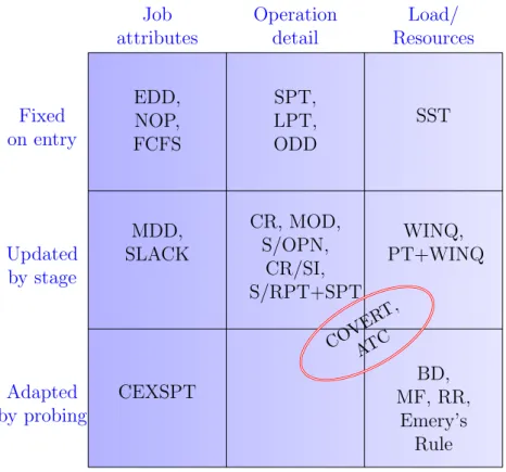
2.1 Classification Matrix of PDRs, adapted from (Kemppainen,2005) . . . 39

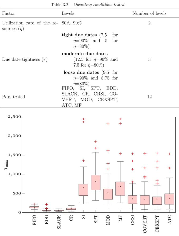
3.1 Box plot of Tmax with (τ,η) = (7.5,90%) . . . 61

3.2 Box plot of Tmax with (τ,η) = (12.5,90%) . . . 62

3.3 Box plot of Tmax with (τ,η) = (15,90%) . . . 63

3.4 Box plot of Tmax with (τ,η) = (5,80%). . . 64

3.5 Box plot of Tmax with (τ,η) = (7.5,80%) . . . 64

3.6 Box plot of Tmax with (τ,η) = (8.75,80%) . . . 65

3.7 Tardiness distribution for rules of set 1 with corresponding (τ,η) . . . 66

3.8 Tardiness distribution for rules of set 2 with corresponding (τ,η) . . . 67

3.9 Comparison of Tmax and Trms for rules of set 1 . . . 68

3.10 Comparison of Tmax and Trms for rules of set 2 . . . 69

3.11 Comparison of Tmax and Trms for other rules . . . 70

5.1 The proposed framework . . . 90

5.2 Simulation Module . . . 91

5.3 An Example of Generating Decision Tree from a Simple Training Block . . 93

5.7 System Performance for ¯T . . . 104

5.8 Box Plot of ¯T for Test Instances . . . 105

5.9 System Performance for Tmax . . . 106

1

List of Tables

1.1 Some Performance Measures . . . 15

1.2 An example problem to illustrate Regular measure. . . 16

1.3 An example problem to illustrate classes of schedules . . . 20

1.4 Some examples for the field α . . . 23

1.5 Some examples for the field β . . . 26

1.6a Some examples for the field γ . . . 26

1.6b Some MO examples for the field γ . . . 27

1.7 An instance of a JSSP . . . 28

2.1 Relevant Literature Review on PDRs . . . 40

3.1 Simulation model parameters . . . 59

3.2 Operating conditions tested. . . 60

3.3 Confidence Interval for Correlation between Tmax and Trms . . . 71

4.1 Review of Literature . . . 83

5.1 An Instance from the Test Data Set . . . 96

5.2 Experimental Setup . . . 98

5.3 Selected Attributes for Tmax . . . 99

5.4 A partial list of inferred rules for ¯T . . . 101

5.5 A partial list of inferred rules for Tmax . . . 102

1

GLOSSARY OF NOTATION

Oj Set of operations of jth job

♯ Cardinality of a set

f Set of Objectives

C Set of Constraints

Jj jth job

Mk kth machine

Ojk An operation of jth job to be processed on kth machine

Oj(i) ith operation of job Jj

Indices

j Index for job, jth _job

k Index for machine, kth_machine

i Index for operation, ith _{operation of a given job}

j,j Indexes for jobs

u,v Indexes for operations

Job Attributes

rj Ready time, Ready time of jth job

sj Start time of jth job

pj Total processing time of jth job

dj Due date of jth job.

˜

dj Dead-line of jth job

Cj Completion time of jth job

oj Total number of operations of jth job.

Lj Lateness of jth job

Tj Tardiness of jth job

̺j Remaining processing time of jth job

ςj Slack of jth job

Operation Attributes

pj(i) Processing time of ith operation of jth job

dj(i) Due date of ith operation of jth job

sj(i) Service start time of ith operation of jth job

Cj(i) Completion time of ith operation of jth job

pjk Processing time of an operation of jthjob to be processed

on kth _machine

djk Due date of an operation of jth job to be processed on

kth _machine

sj(i) Service start time of an operation of jth job to be

pro-cessed on kth _machine

Cjk Completion time of an operation of jth job to be

proces-sed on kth _machine

Wj(i) Expected waiting time for ith operation of jth job

System parameters/Variables

t Current time

π A processing sequence

σ A schedule

τ Due-date tightness factor

ρ Due-date range

m Number of machines

n Number of jobs

nt Number of jobs in system at time t

µx Mean of x

E(x) Expectation of x

V ar(x) Variance of x

(x)+ _max(x,0)

1

Introduction

Over the last fifty years, scheduling theory has evolved as a major active area of research attracting a wide spectrum of researchers ranging from computer and management scien-tists to production engineers. There exist a significant amount of literature on a wide variety of methods to solve different scheduling problems. These methods range from industry-standard dispatching rules to state-of-the-art meta-heuristics and sophisticated optimization algorithms.

Scheduling is concerned with solving a Constraint Optimization Problem (an optimization problem with finite solution space for each of its instance (Colorni et al., 1996)).

The job shop problem is considered as one of the most general and well developed schedu-ling problems with much practical significance. The problem is generally NP-hard (Non-deterministic Polynomial-time hard) except for a very few special cases. Conway et al. (1967) describes the problem as a fascinating challenge that is extremely hard to solve despite its quite simple structure. The reason for computational intractability of job shop scheduling problem is mainly its combinatorial nature besides many conflicting factors that must be taken into account (Zobolas et al., 2008).

The history of solving job shop scheduling problem encompasses a wide spectrum of approaches. Initially, the focus of researchers remained on the exact approaches. These include the earlier efficient methods, mathematical methods and enumerative techniques. Branch and bound are considered among the most successful exact methods, however they demand phenomenal computing time to obtain an optimal solution (Zobolas et al., 2008). Later on, an era of heuristic methodologies is observed, although simple dispatching rules were already in use. Various bottleneck-based heuristics are developed during this period. Thereafter, with the emergence of more sophisticated meta-heuristics and

tech-niques based on artificial intelligence, substantial progress is made in late 80s and early 90s (Jain and Meeran, 1998). Powerful meta-heuristics coupled with the computational power of modern computer systems enabled to make use of these approaches on relatively larger problems. However, Lawrence and Sewell (1997) found that the performance of these so-lution methodologies deteriorates due to processing time uncertainty when compared to dynamically updated heuristic schedules.

In dynamic scheduling, jobs are continually revealed during the process of schedule exe-cution. Dynamic scheduling is closely related to real-time control, as decisions are to be made based on the current state of the system. This on-line aspect greatly influences the scheduling decisions as the schedule creation and schedule execution no longer remain two different processes. Scheduling decisions are to be made in a very short time as the time required to generate a schedule becomes relatively more important factor than merely finding a best quality schedule in an extended period of time. Moreover, schedule is requi-red to be highly reactive to cope with unanticipated circumstances. Priority dispatching rules are considered as the best choice in such an environment mainly due to their ease of implementation and intuitive appeal despite their poor performance in most of the scheduling problems.

The priority dispatching rules based approach is the simplest and most used approach in practice for dispatching jobs in real-time for processing on machines. Numerous studies have been made on the nature, effectiveness and performance of different priority dis-patching rules under varying scheduling conditions. Panwalker and Iskander (1977) has reviewed 113 priority dispatching rules while new rules are continuously emerging. Howe-ver, there is still a lack of satisfactory results in literature on the performance of priority dispatching rules that would have lead to extensive real-world applications. Unfortunately, the superiority of one scheduling rule to the other is not obvious and often conflicting re-sults have been reported possibly due to different conditions and parameter-settings used for the scheduling environment. Moreover, the performance of priority dispatching rules is dependent on the performance criterion. An apparently highly efficient rule in regards with one performance criteria may give very poor results for some other performance crite-rion even under the same conditions. Even for the pragmatic priority scheduling approach, the overall performance of priority dispatching rules diminishes due to the dynamic and stochastic nature of the system.

Under the general title of Artificial Intelligence (AI), a series of new techniques emerged in early 80s to solve the job shop scheduling problem (Jones and Rabelo, 1998). They in-clude expert/knowledge-based systems, artificial neural networks and inductive learning. These techniques generally employ both the quantitative and qualitative knowledge

spe-5 cific to problem domain as well as procedural knowledge of the solving methods. These approaches are assumed to capture complex relationships and transform them into elegant data structures for subsequent generation of heuristics. The heuristics obtained however, are quite complex in most of the cases, as compared to priority dispatching rules. Moreo-ver, systems based on these techniques are too time-consuming to build and quite complex to maintain.

Knowledge acquisition is the basic step in developing the knowledge-base. The knowledge source is usually a human expert, the simulation data or the historical data. A machine learning technique employs this data as a set of training examples. These training examples are used to train the machine-learning algorithm to acquire knowledge about the manufac-turing system (Michalski et al., 1986, 1998). Intelligent decisions are then made (such as selecting the best rule for each possible system state) in real time, based on this knowledge (Nakasuka and Yoshida, 1992; Shaw et al., 1992; Yeong-Dae, 1994; Min and Yih, 2003).

The major drawbacks of priority dispatching rules include their performance-dependence on the state of the system and non-existence of any single rule, superior to all the others for all possible states the system might be in (Geiger et al., 2006). Meta-heuristics (e.g. simulated annealing and tabu search) have an advantage over the priority dispatching rules in terms of solution quality and robustness, however these are usually more difficult to implement and tune, and computationally too complex to be used in a real time system. Robust and better-quality solutions provided by meta-heuristics contain useful knowledge about the problem domain and solution space explored. Such a set of solutions represents a wealth of scheduling knowledge to the domain that can be transformed in a form of decision tree or a rule-set. In this work, we propose an approach to exploit this scheduling knowledge.

The proposed data mining-based approach discovers previously unknown dispatching rules for job shop scheduling problem. An efficient meta-heuristic such as tabu search can provide robust and better-quality solutions for a job shop scheduling problem that contains useful knowledge about the problem domain and solution space explored. A set of such solutions for different instances of a job shop scheduling problem represents a wealth of scheduling knowledge to the domain. The idea is to exploit this scheduling knowledge and to transform it in a form of decision tree or a rule-set. The rule-set may then be used as a standard dispatching rule at the waiting lines of a job shop in an on-line manner.

Thesis Organization

This thesis report is composed of five chapters. The first chapter presents the scheduling problem and the basic concepts in the field of scheduling. The key elements, of which of shop scheduling problem is composed as well as the notations used to characterize the problem are recalled. Thereafter, we present different classes of schedules. Classification of scheduling problems are then presented in order to distinguish different combinations of scheduling environments, conditions and objectives. This follows with a formal definition of job shop scheduling problem. Then the schedule visualization by Gantt diagram and the scheduling problem representation using disjunctive graph formulation is described. Finally, a general introduction to different methods used in solving job shop scheduling problems are discussed.

The second chapter provides a state-of-the-art review on priority dispatching rules in context with job shop scheduling environment. Frequently used classification schemes for these pdrs found in literature are reviewed. This follows with a detailed discussion on the structure and characteristics of most frequently used pdrs in literature.

In the third chapter, a simulation based analysis of tardiness based performance measures for a set of frequently used pdrs is made in order to highlight the similarities/dissimilarities in the behavior of pdrs. Tardiness based performance measures focus on different aspects of a very important class of objectives in a manufacturing system. The first part of the chapter presents these different tardiness based performance measures. These performance measures are not independent of each other. Moreover, the relation among these perfor-mance measures is generally not obvious even for simple scheduling strategies such as priority dispatching rules. Based upon the behavior of different priority dispatching rules in regards with these performance measures, we identify two sets of pdrs using the distri-bution of the maximum tardiness (i.e. Tmax), a very important measure representing the

worst case behavior. The worst-case behavior in regards with tardiness is very difficult to identify due to its value at a single-point only. However, it is possible to establish some guidelines in predicting this worst-case behavior in regards with tardiness as well as the width of the tardiness by evaluating root mean square tardiness (Trms). Results showing

the correlation among two very important measures, maximum tardiness (Tmax) and root

mean square tardiness (Trms) are presented along-with discussion on these results.

In chapter 4, a state-of-the-art survey on the application of learning based approaches in the field of job shop scheduling is given. It provides an effective overview of the chal-lenges and benefits related to the application of learning algorithms in solving scheduling problems. The survey reveals that their is a lack of systematic use of the scheduling

know-7 ledge despite the fact that the approach has been acknowledged by most of the authors as promising in scheduling domain. Moreover, it is generally not obvious how much a certain set of scheduling data is relevant to the scheduling environment for desired ob-jectives. The emergence of data mining has invoked the academic interest in analyzing the complex problems like this in a more methodical way. A brief review of the factors affecting the performance of inductive learning algorithm, for example feature selection and discretization is given in the last part.

A data mining based approach to discover previously unknown priority dispatching rules for job shop scheduling problem is presented in chapter 5. In the beginning, a brief des-cription of some necessary background areas such as tabu search and data mining is given. Then the proposed framework is presented along with the structure and functional de-tails of the different modules. The approach is based upon seeking the knowledge that is assumed to be embedded in the efficient solutions provided by the optimization module, built using tabu search. The objective is to discover the scheduling concepts using data mining and hence to obtain a set of rules capable of approximating the efficient solutions for a job shop scheduling problem (JSSP). The data mining based scheduling framework is implemented for a job shop problem with mean tardiness and maximum lateness as the scheduling objectives. The results indicate the superior performance of the proposed system relative to a number of priority dispatching rules and hence proves to be promising approach.

1

Scheduling: A General

Introduction

1.1 Introduction . . . 10

1.2 Elements of a Scheduling Problem . . . 11

1.2.1 Jobs . . . 11 1.2.2 Resources . . . 11 1.2.3 Constraints . . . 12 1.2.4 Objectives. . . 13 1.3 Classes of Schedules . . . 18 1.3.1 Feasible schedule . . . 19 1.3.2 Semi-active schedule . . . 19 1.3.3 Active schedule . . . 19 1.3.4 Non-delay schedule . . . 20 1.3.5 Optimal schedule . . . 20

1.4 Classification and Notations of Scheduling Problem . . . 22

1.4.1 αfield:. . . 22 1.4.2 β field:. . . 25 1.4.3 γfield:. . . 25 1.5 Scheduling Phases . . . 27 1.5.1 Predictive Phase . . . 27 1.5.2 Reactive Phase . . . 27

1.6 Job Shop Scheduling Problem . . . 27

1.6.1 Formal definition of JSSP . . . 28 1.6.2 Graphical Representation . . . 28 1.7 Solving Methods . . . 29 1.7.1 Exact methods . . . 30 1.7.2 Approximation methods . . . 30 1.8 Conclusions . . . 32

This chapter presents an overview of the scheduling domain and related concepts. The key elements of shop scheduling problem and notations are presented. Different shop scheduling environments along with classification of shop scheduling problems is given. A

formal definition of job shop scheduling problem (JSSP) and its representation are given. Then a general introduction to different approaches used in solving JSSP are discussed.

1.1

Introduction

Scheduling is a decision-making process that is extensively encountered in a large variety of systems. However it is widely used in manufacturing systems where it is generally referred as machine scheduling. Machine scheduling is one of the most important issues in the planning and operation of manufacturing systems. It is aimed at efficiently allocating the available machines to jobs, or operations within jobs and subsequent time-phasing of these jobs on individual machines (Shaw et al., 1992).

A solution to a scheduling problem represents a schedule (σ) that satisfies all the constraints of the problem. A schedule is composed of following three major processes: assignment : It is a process of allocating a machine to each task to be executed.

sequencing : It is the process of assigning an order of execution of the tasks on each machine.

timetabling : It is the process of assigning a start time and finish time to each task.

However, these three processes may be dealt as separate problems, known as assignment problem, sequencing problem and timetabling problem respectively (French, 1982).

Scheduling problems are generally very complex in nature due to their combinatorial na-ture. However these problems are extensively studied in literature as benchmark problems for the optimization methods apart from their own practical applications. Traditional ap-proaches to solve scheduling problems use simulation, analytical models, heuristics or combination of these methods.

Different components of a scheduling problem are the tasks, constraints, resources and the objective functions. In the following, these key elements of a scheduling problem are presented.

1.2 Elements of a Scheduling Problem 11

1.2

Elements of a Scheduling Problem

A scheduling problem is a typical representative of a combinatorial optimization class of problems consisting of a set of jobs J , a set of resources M, a set of objectives f and a set of constraints C.

1.2.1

Jobs

A job Jj is a fundamental entity described in time domain by a start time and

fi-nish time, that is executed for a processing time on one or more resources/machines (Esquirol and Lopez, 1999).

Each job Jj consists of oj number of operations, {Oj(1),Oj(2),...,Oj(oj)} with each operation, Oj(i) ( or Ojk) to be processed on a machine Mk during a processing time pjk. A job is

associated with a release date, rj, specifying the time before which no operation of the job

can be processed, a processing time, pj(= Pn_j=1pj(i)), the time for which the job executes

on machine(s) and a due date, dj, the date at which job is promised to be completed.

The completion time of a job, Cj, is by which all the operations of the job complete its

execution on corresponding machines. Number of jobs in the problem is denoted as n (= ♯J ) while number of jobs available for processing at any instant t, is denoted as nt.

Total number of operations, Pn

j=1oj (= ♯O) in a scheduling problem generally reflect the

problem size.

1.2.2

Resources

A resource, Mk is any physical or virtual entity of limited capacity and/or availability,

allocated to the execution of jobs competing for it.

The term machine is generally used instead of resource in shop scheduling literature. There are different types of resources. A resource can be classified as renewable and consumable. Renewable resources become available again after use with the same capacity, while consumable resources lose their capacity or disappear after use (Kind’t and Billaut, 2006).

Resources can also be classified as cumulative or disjunctive. Cumulative resources are capable of processing more than one task in parallel while disjunctive resources can process only one task at a time. Usually a limit on the capacity of the resources is the major constraint besides others.

In this study, only renewable disjunctive resources are taken into account. Number of machines denoted as m (= ♯M), also reflect the size of a scheduling problem.

1.2.3

Constraints

A constraint represents a restricted set of value that can be taken by a decision variable involved in the problem. A solution of a scheduling problem must always satisfy the given constraints. A solution that violates any of the constraints is not a feasible solution. Constraints can be classified as temporal constraints and resource-capacity constraints.

Temporal Constraints

Temporal constraints are generally related to execution window of a job (or operations) in time horizon. These constraints specify absolute position, relative position or structure of this execution window.

0 1 2 3 4 5 6 7

Mk J_j

(a) Feasible schedule

0 1 2 3 4 5 6 7

Mk J_j

(b) Infeasible schedule

Figure 1.1 – Temporal constraint: Absolute position and size of execution window Temporal constraints specify absolute position of the execution window for a job in time horizon. This means that a job Jj can not start its execution before rj and must finish its

processing before ˜dj. It may be specified as

rj 6sj,Cj 6 ˜dj,

where sj is the time at which jth job starts its execution. Figure 1.1 illustrates the

exe-cution of a job Jj with ready time rj = 0 and dead-line ˜dj = 5. Figure 1.1(a) shows a

feasible schedule with respect to this constraint whereas an infeasible schedule is shown in Figure 1.1(b).

1.2 Elements of a Scheduling Problem 13 Temporal constraints may also specify the relative positions of execution windows of dif-ferent jobs on the same machine (known as precedence constraints), e.g. for the constraint that Ogk must precede job Ohk (i.e. Ogk → Ohk) can be expressed as

Cgk 6shk.

Temporal constraints specify the structure of this execution window i.e. whether it must be in an integral form for an operation or may be split (preemption) on time scale. Resource Constraints

These constraints specify the capacity and/or availability of a resources. They are also referred as disjunctive constraints in the case of renewable resources. This means, for example, that no more than one operation can be executed at the same time on a resource of unit capacity. This type of constraint is expressed as

∀u,v ∈ O, M(u) = M(v) ⇒ Cu 6sv or Cv 6su.

1.2.4

Objectives

An objective reflects the desired characteristics in the solution to find, for a scheduling problem by executing a given set of tasks on the machines in a certain sequence.

Generally, there are more than one possible solution to a problem. Each solution of the problem has its own characteristics. The objectives take into account these characteris-tics, for preferring one solution to the other. In some cases it is not possible to find all the required characteristics in a single solution. However, in such cases some of the prefe-rences may be relaxed to find the solution of the problem with relatively more important characteristics, reflecting the objectives.

The objectives reflect the characteristics desired in the final schedule. Different perfor-mance measures may be used for the evaluation of schedules in regards with the objectives under consideration. These may be based upon completion times, due dates or inventory, utilization costs etc.. Performance measures specify the extent to which the desired ob-jectives are achieved. Two performance measures are equivalent if a schedule which is

optimal with respect to one is always optimal with respect to the other as well and vice versa (French, 1982).

The two large families of objectives are:

– minimax, which represent the maximum value of a set of functions to be minimized, and

– mini-sum, which represent a sum of functions to be minimized.

The most studied objective related to completion times is minimizing the completion time of the entire schedule, known as makespan and denoted as Cmax. It is defined as

Cmax= max 16j6nCj.

Cmax is one of the flow time based objectives where flow time of a job Jj is defined to

be the time that the job spends in the shop (French, 1982), and is represented as Fj.

Mean flow time ( ¯F ) and maximum flow time (Fmax) are among other flow time based

performance measures that are often used in scheduling problems. These measures are defined respectively as follows:

¯

F = ΣjFj n , Fmax= max

16j6nFj.

An objective may also be a function of the due dates. One of the basic functions involving due dates is lateness. The lateness of job j is defined as Lj = Cj−dj, which is positive when

job j is completed late and negative when it is completed early. An important example of performance measure using lateness is maximum lateness, Lmax. It is defined as

Lmax = max 16j6nLj.

Another very important function of due dates is tardiness, which can be measured through several performance measures. The tardiness of a job is computed as

Tj = max(0,Lj).

1.2 Elements of a Scheduling Problem 15 It is defined as

¯

T = ΣjTj n .

Maximum tardiness, Tmax is another very important tardiness based measure that is

equi-valent to Lmax and defined as

Tmax = max 16j6nTj.

It can be of great interest for the decision-maker in the shop as an indication of the worst case behavior during a particular experiment.

The number of tardy jobs is defined as,

Uj =        1 if Lj > 0 0 otherwise

There is a unit penalty for each tardy job. It does not consider the amount of tardiness involved for any job. An equivalent measure namely percentage tardiness (%T = ΣUj/n ×

100) is also used extensively in literature. The conditional mean tardiness described as

CM T = ΣjTj ΣUj

.

measures the average amount of tardiness for the completed jobs which are found to be tardy.

Name Notation Regular Type

Makespan Cmax yes minimax

Maximum tardiness Tmax yes minimax

Total tardiness ΣjTj yes mini-sum

Mean tardiness T¯ yes mini-sum

Conditional mean tardiness CMT no mini-sum

Total weighted tardiness P

jwjTj yes mini-sum

Performance measures can be classified into regular ones and those that are not. A regular measure of performance is one that is non-decreasing in the completion times C1,...,Cn.

Thus R is the function C1,C2, . . . ,Cn such that

C1 6C1′,C2 6C2′, . . . ,Cn6Cn′, together

⇒ R {C1,C2, . . . ,Cn} 6 R {C1′,C2′, . . . ,Cn′}.

Maximum completion time (Cmax) and mean tardiness ( ¯T ) are examples of regular measure

whereas CM T is not a regular one. Table 1.1 lists a few performance measures.

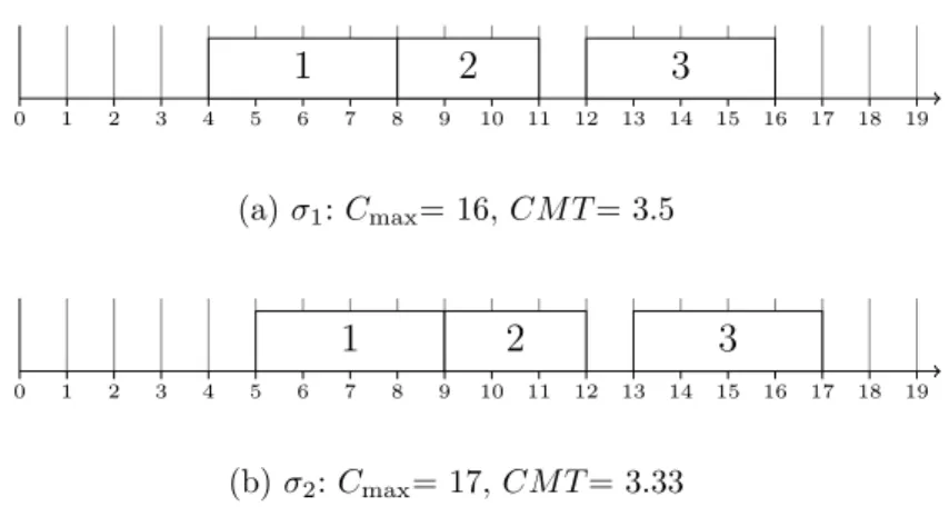
Two different solutions are illustrated in Figure 1.2 for problem of Table 1.3. If we com-pare, for example, the σ1 and σ2 schedules, although Cmax is higher for the σ2 schedule,

the CM T obtained is less for this schedule, i.e. Cmax(σ1) 6 Cmax(σ2) does not imply

CM T (σ1)6CM T (σ2). Hence CM T is a non-regular measure.

j rj pj dj

1 0 4 8

2 2 3 8

3 4 4 12

Table 1.2 – An example problem to illustrate Regular measure

0 1 2 3 4 5 6 7 8 9 10 11 12 13 14 15 16 17 18 19 1 2 3 (a) σ1: Cmax= 16, CM T = 3.5 0 1 2 3 4 5 6 7 8 9 10 11 12 13 14 15 16 17 18 19 1 2 3 (b) σ2: Cmax= 17, CM T = 3.33

Figure 1.2 – Schedules for problem in Table 1.2illustrating performance measures

Single Objective Optimization

In a single objective scheduling problem, it is desired to find a feasible schedule with the best possible quality of only one objective. Majority of the literature on scheduling tackles

1.2 Elements of a Scheduling Problem 17 the problems with a single objective.

Multi-objective Optimization

Generally, single objective scheduling problems make the major part of the literature in machine scheduling domain. However, it is often desired to have multiple preferences for a solution to find. These preferences may lead to conflicting objectives. Thus maximizing one objective may degrade the other objectives to an unacceptable level. It is required to find a compromise solution, satisfying all given objectives simultaneously, although may not be optimal with respect to a single objective.

Multi-objective (MO) optimization is the process of simultaneously optimizing two or more objectives subject to certain constraints. A multi-objective optimization problem is defined by (Ehrgott and Gandibleux, 2000) as

min f (x), x ∈ X, where f (x) = [f1(x),f2(x),...,fp(x)]T

with each f (x) ∈ Y , p being the number of objectives, X is the set of all possible solutions and Y is the objective space.

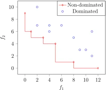
We speak of dominance of solutions as the way to compare the solutions of a multi-objective problem. If x1,x2 ∈ X and ∀k,fk(x1) 6 fk(x2), with at least one strict inequality,

we say x1 dominates x2 (x1 ≻ x2) and f (x1) dominates f (x2). A feasible solution ˆx ∈ X

is efficient or Pareto optimal if there is no other x ∈ X such that ∀k,fk(x) 6 fk(ˆx) with

at least one strict inequality, i.e. there is no solution at least as good as x. As ˆx is efficient then f (ˆx) is called non-dominated point (Ehrgott and Gandibleux, 2000). It is generally required to generate a set of efficient solutions. The set of all efficient solutions is denoted by XE, the representation of XE in objective space is called the efficient frontier or Pareto

front, and the set of all non-dominated points ˆy = f (ˆx) ∈ Y by YE. Figure 1.3 illustrates

the difference between dominated and non-dominated solutions in a bi-objective space. There are different approaches, found in literature to solve multi-objective optimization problem.

– Weighted sum approach: In this approach, a multi-objective problem is trans-formed into single objective problem by aggregating all the objectives. This single objective problem is then solved repeatedly with different parameter values. This is the most commonly used technique to find XE. XE can be partitioned into supported

0 2 4 6 8 10 12 0 2 4 6 8 10 f1 f2 Non-dominated Dominated

Figure 1.3 – A bi-objective space with dominated and non-dominated solutions

x ∈ XSE is an optimal solution of the following parameterized single objective

pro-blem for some non-negative λ = (λ1,λ2,...,λp),∀k

min x∈X p X k=1 λkfk(x).

– ǫ-constraint approach: The ǫ-constraint method is another technique to solve multi-objective optimization problems that consists of minimizing one of the objec-tives with an upper bound constraints on the other objecobjec-tives.

– Lexicographic approach: In this approach, the objectives are ranked in a cer-tain priority order and then optimized in that order without degrading the already optimized objectives.

– Pareto approach: This approach is aimed at generating the complete set of efficient solutions.

1.3

Classes of Schedules

Assumptions have to be made with regard to what the scheduler may or may not require when he generates a schedule. For example, it may be the case that a schedule must not have any unforced idleness on any of the machines or vice versa.

The schedule space can be partitioned into subclasses on the basis of how different ope-rations are executed on the time horizon. These classes help to rank different schedules

1.3 Classes of Schedules 19 according to some regular performance measure. Figure 1.4 illustrates the schedule space of these classes as a Venn diagram for a regular performance measure.

1.3.1

Feasible schedule

A schedule is feasible if the execution order of all the jobs respect all the specified constraints of the scheduling problem.

1.3.2

Semi-active schedule

A semi-active schedule is a left-aligned feasible schedule where no task can be shifted to its left without changing the order of operations and without delaying any other operation. Hence it is not possible to finish an operation earlier on a machine without reordering tasks. In such a schedule the only way to improve the makespan is by reordering the sequence of operations on the machines. For each processing sequence, there exists a unique semi-active schedule (French, 1982). On the Gantt diagram, such a schedule may be seen as a schedule where no sliding of a block to its left is possible.

1.3.3

Active schedule

A feasible schedule is active if no operation can be processed earlier without delaying the starting date of another operation. This means that the schedule is left-shift and there in not enough room available between any two jobs where some other job may be inserted without violating any of the constraints. An active schedule is necessarily a semi-active schedule as well. To minimize a regular measure of performance it is sufficient to consider active schedules only.

On Gantt diagram, it may be seen as schedule where there is neither the possibility of sliding a block to its left, nor the leap frogging of a block to its left is possible. Of course, generating an active schedule for a given processing sequence may alter the sequence of operations, if there is possibility of leap-frogging.

Non-delay Semi-active

Active Feasible

Optimal

Figure 1.4 – Classes of Schedules

1.3.4

Non-delay schedule

A schedule is called non-delay if no machine is kept idle while an operation is waiting for being processed on that machine. A non-delay schedule is necessarily an active schedule and hence semi-active as well.

1.3.5

Optimal schedule

An optimal schedule is a schedule that gives the best possible value for some given perfor-mance measure. There may be more than one optimal schedules for the same perforperfor-mance measure. For more than one objective, the sense of optimality is quite different as explai-ned in § 1.2.4. Note that at least one optimal schedule is active, however there need not be an optimal schedule, which is non-delay.

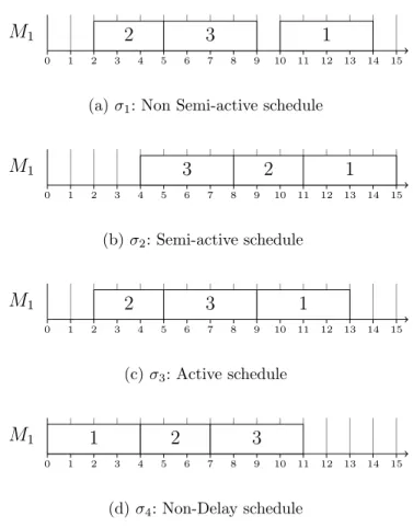
Consider an example of a single machine problem with three single-operation jobs as given in Table 1.3. Figure 1.5 illustrates these classes of schedules for this simple problem. Schedule σ1 (Figure 1.5(a)) is not a semi-active schedule, because job 1 starts at t = 10,

j rj pj

1 0 4

2 2 3

3 4 4

1.3 Classes of Schedules 21

0 1 2 3 4 5 6 7 8 9 10 11 12 13 14 15

M1 2 3 1

(a) σ1: Non Semi-active schedule

0 1 2 3 4 5 6 7 8 9 10 11 12 13 14 15 M1 3 2 1 (b) σ2: Semi-active schedule 0 1 2 3 4 5 6 7 8 9 10 11 12 13 14 15 M1 2 3 1 (c) σ3: Active schedule 0 1 2 3 4 5 6 7 8 9 10 11 12 13 14 15 M1 1 2 3 (d) σ4: Non-Delay schedule

Figure 1.5 – Schedules of the problem described in Table1.3

that could have started at t = 9 without violating any constraint, and without changing the execution order of jobs on the machine. Since this ordering is not semi-active, it is neither active nor non-delay.

Schedule σ2 (Figure 1.5(b)) is a semi-active schedule as no job can be slid towards its

left without reordering the tasks. It is not an active schedule. In fact, if job 3 is at first position, the schedule can never be active as there will always be a room for job 1 before job 3. As it is not active, so it is also not non-delay.

Schedule σ3 (Figure 1.5(c)) is an active schedule (and a semi-active as well) because no

job can be shifted towards its left without delaying other tasks. It is however, not a non delay schedule as job 1 could have been processed on machine at t = 0, but machine is kept idle.

Schedule σ4 (Figure 1.5(d)) is a non-delay (as well as active and semi-active) as machine

1.4

Classification and Notations of Scheduling

Pro-blem

Based on the job arrival process, scheduling problems in which number of jobs are known and fixed with all jobs having the same ready times are referred as static problems in contrast to the dynamic problems in which jobs are continually revealed during the exe-cution process (French, 1982).

Scheduling problems with all the variables describing the problem data (e.g. process times) are known a priori are termed as deterministic problems in contrast to stochastic schedu-ling problems where these variables are probabilistic in nature.

Scheduling problems can have single stage and multi-stage environments. In a single stage environment, each operation goes through one machine only. In a multi-stage environment, an operation can be executed by one of the machines of the same stage, so a machine has to be selected first to perform the operation (Pinedo and Chao, 1999).

There are different notations used to classify scheduling problems. (Conway et al., 1967) formulated a four field notation, A/B/C/D which is suitable for basic scheduling pro-blems. In this notation, the field A represents number of jobs, B represents number of machines, C represents the shop environment and D represents the scheduling objective. MacCarthy and Liu (1993) improved this notation by proposing several modifications to C descriptor. Graham et al. (1979) proposed a three field notation α, β and γ. This is the most used descriptive method to represent a scheduling problem.

1.4.1

α field:

The α field describes the machine environment. It consists of α1 and α2 where α1 is the

type of shop and α2 is the number of machines in the problem and is optional. If this field

is empty, then the number of machines is the data of the problem. Some notations of α field are given in Table 1.4.

Machine environments can be classified in two categories. In the first category, each job requires one and only one machine. Single machine, identical parallel and unrelated parallel machine environments fall into this category. In the second category, there are m different work-centers with each work-center consisting of one or many parallel machines. Each job Jj ∈ J consists of a set of operations Oj. Depending upon the routing policy of

1.4 Classification and Notations of Scheduling Problem 23

Table 1.4 – Some examples for the field α

α Description

φ Single machine, the value for the field α is “1” P m m Identical parallel machines

Qm m Parallel machines with different speeds Rm m Unrelated parallel machines

F m m machine flow shop

F F c c stages in series as a flow shop with each stage as P m or Qm Fπm Permutation flow shop of m machines

Jm m machine job shop

F Jc c work-centers with each work center as Pm or Qm Om m machine open shop

these operations on the machines, three different classes of machine environments can be identified.

Flow shop

All jobs are to be processed sequentially on multiple machines where each job has to follow the same route. Figure 1.6 demonstrates a three machine flow shop. A generalization of flow shop is the flexible flow shop that consists of a number of stages in series with a number of machines in parallel at each stage. There exist many variants of the flow shop e.g. zero-buffer flow shop, flow shop with blocking, no-wait flow shop and the hybrid flow shop. Academic research, however is more focused on a simplified version of flow shop, the permutation flow shop where jobs are to to be processed in the same sequence by each of the machine. A permutation flow shop is illustrated in Figure 1.7.

{J }n

j=1

M

M

M

Figure 1.6 – A three machine flow shop, F 3

Job shop

In a job shop, each job has its own predetermined route to follow. It is a generalization of a flow shop (A flow shop is a job shop in which each job has the same route). Job shop

M

M

M

Figure 1.7 – A three machine permutation flow shop,F 3|prmu|−

has a special precedence relation of the form Oj1 → Oj2 → Oj3 → . . . Ojoj,∀j ∈ J . A generalization of the job shop is the flexible job shop with work-centers that have multiple machines in parallel. Each job visits each machine at most once, however in a variant of job shop, called recirculation job shop, a route may not go through all machines however a job may have multiple visits on a machine for execution of its operations. The latter case is represented by a rcrc entry in the β-field. A flexible job shop with recirculation is considered the most complex machine environment from combinatorial point of view, and is very common in semiconductor industry (Pinedo and Chao, 1999). Figure1.8illustrates a simple job shop with three machines.

J1

M

M

M

Figure 1.8 – A three machine job shop, J3

1.4 Classification and Notations of Scheduling Problem 25 given in § 1.6.

Open shop

In an open shop, there is no predefined sequence of operations among jobs i.e. jobs do not have a predefined routing, instead it is established during the scheduling.

In a mixed shop, the machine routes of jobs can either be fixed or unrestricted. It can be regarded as a mix of aforementioned shops.

1.4.2

β field:

The β field describes the constraints and particularities of the problem. For example: Deadline These are imperative due-dates. A deadline is a due date for which tardiness

is not allowed.

Preemption Processing of a job on a machine may be interrupted and resumed at a later time even on a different machine and already processed amount is not lost. Precedence One or more jobs have to be completed before another job is allowed to

start.

Release Date The release date of job Jj, is the time when a job is arrived at the system

to be processed and the job cannot start its processing before release date. Some possible entries of β field and their notations are given in Table 1.5.

Any other entry that may appear in the β field is self-explanatory. For example, pj = p

implies that all processing times are equal and dj = d implies that all due dates are equal.

Due dates, in contrast to release dates, are usually not explicitly specified in this field; the type of objective function gives sufficient indication whether or not the jobs have due dates.

1.4.3

γ field:

The γ ∈ {fmax,P f } field describes the objective function and is similar to the D

Table 1.5 – Some examples for the field β

β Value Description

β1

pmtn, φ pmtn: preemption is allowed

φ: preemption is not allowed β2

res♯, φ res♯: ♯ limited number of resources φ: no resource limitation

β3

prec, tree, φ

prec: a precedence relation between jobs is speci-fied

tree: a tree like precedence relation between jobs is specified

φ: no precedence relation β4

rj, φ

rj: release dates are specified

φ: ∀j, rj = 0

β5

J 6 p, φ J 6 p: all jobs have at most p operations φ: no restrictions on size of jobs

β6

pjk = 1, a 6 pjk 6b, φ

pjk = 1: each operation has a unit processing time

a 6 pjk 6b: processing time of each operation has

a lower bound a and an upper bound b φ: no restriction on processing times

Table 1.6a – Some examples for the field γ

γ Description

Cmax Makespan

Tmax Maximum tardiness

ΣjTj Total tardiness

¯

T Mean tardiness

Some are given in Table 1.6a. For multi-objective problems, list of objectives separated by comma are used in γ field. For instance, a single machine problem with Cmax and ¯T

can be noted as 1||Cmax, ¯T . Moreover, based on the method to compute Pareto optimum,

1.5 Scheduling Phases 27

Table 1.6b – Some MO examples for the field γ

γ Description

♯(f1,...,fK) Enumeration of non-dominated solutions

Lex(f1,...,fK) Lexicographic optimisation of K objectives

Fl(f1,...,fK) Convex combination of K objectives

ǫ(f1,...,fK) ǫ-constraint method of K objectives

1.5

Scheduling Phases

1.5.1

Predictive Phase

The phase of a scheduling method that takes place before the actual execution of the schedule is referred as predictive phase. This phase of the scheduling method is generally not time constrained in terms of finding the solution and is applied to the model of the real system as an off line method.

1.5.2

Reactive Phase

The reactive phase of a scheduling method takes place during the execution of the schedule. The scheduling method during this phase, therefore can observe the occurrence of actual events of the system. However the scheduling method during this phase must not be too time consuming.

1.6

Job Shop Scheduling Problem

Our focus in this study is on a specific scheduling environment, namely job shop. Here we shall describe the formal definition of a job shop scheduling problem (JSSP), graphical representation, its complexity, different benchmark problems and a brief overview of resolution approaches for JSSP.

1.6.1

Formal definition of JSSP

The job shop scheduling problem with multiple precedence constraints is a combinatorial optimization problem composed of a finite set J of n jobs {Jj}n_j=1 to be processed on a

fi-nite set M of m resources {Mk}m_k=1. A job Jj consists of a sequence Oj = (Oj1,Oj2,...Ojoj) of oj operations with each operation Ojk as part of exactly one job Jj to be processed

during a processing time pjk > 0 on a resource Mk. A resource can execute only one

operation at a time. Solving a job shop problem is the task of assigning each operation, a specific position on the time scale of specified machine while optimizing a set of given performance measures (Conway, 1965b).

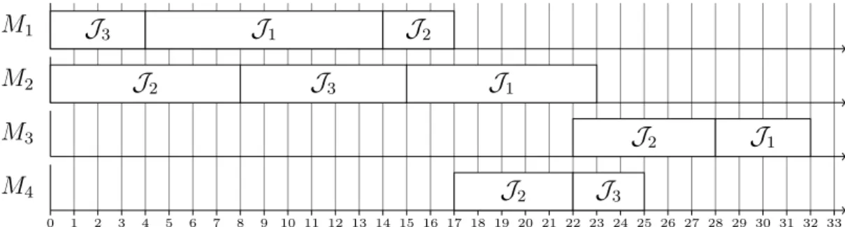
Generally size of the JSSP is given as m × n. An instance of a JSSP is given in table Table 1.7.

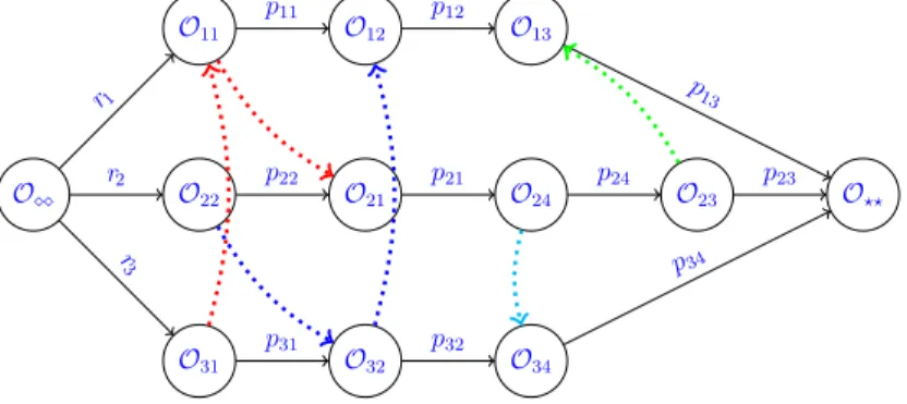
Job rj machine sequence pjk

J1 0 M1, M2, M3 p11=10, p12=8, p13=4 J2 0 M2, M1, M4, M3 p22=8, p21=3, p24=5, p13=6 J3 0 M1, M2, M4 p31=4, p32=7, p34=3 Table 1.7 – An instance of a JSSP

1.6.2

Graphical Representation

Gantt diagram is a very simple and extensively used tool to graphically present the exe-cution order and timings of tasks on the machines throughout the time horizon. Gantt diagram can be machine-oriented or job-oriented. In this study, all the Gantt diagrams will be machine-oriented. An example of a machine-oriented Gantt diagram is shown in Figure 1.9 for an arbitrary feasible solution for the problem instance given in Table 1.7.

1.6.2.2 Disjunctive Graph

Although Gantt diagram is an excellent monitoring tool of a schedule, it is inca-pable of representing the problem itself. Disjunctive graph representation proposed by (Roy and Vincke, 1981) is able to effectively represent a scheduling problem.

1.7 Solving Methods 29 0 1 2 3 4 5 6 7 8 9 10 11 12 13 14 15 16 17 18 19 20 21 22 23 24 25 26 27 28 29 30 31 32 33 M1 J₃ J₁ J₂ M2 J₂ J₃ J₁ M3 J2 J1 M4 J₂ J₃

Figure 1.9 – Gantt diagram for a schedule for the problem in Table 1.7.

A disjunctive graph is a 3-tuple G=(V,C,D) with V as set of vertices representing the set of operations O and two special vertices as a source node and a terminal node, C as set of conjunctive arcs representing the given precedence constraints between the operations of the same job, and set of disjunctive arcs by D={{u,v}|u,v ∈ O,u 6= v,M(u) = M(v)} represent the machine capacity constraints. Each arc has a weight, equal to the processing time of the operation corresponding the vertex from which the arc emits. Figure 1.10

illustrates a disjunctive graph for a job shop problem with four machines and three jobs as given in Table1.7. For even a slightly larger problem, the disjunctive graph representation gets too complicated to visualize. A relatively simplified version the disjunctive graph, where instead of inter-connecting all the operations of the same machine by disjunctive arcs, only one disjunctive arc is drawn, may be used (as shown in Figure1.11). By setting the direction of each arc such that there are no cycles in the disjunctive graph, a solution to the problem is represented, as shown Figure 1.12.

O11 O12 p11 O13 p12 O22 O21 p22 O24 p21 O23 p24 O31 O32 p31 O34 p32 O⋄⋄ r1 r2 r3 O⋆⋆ p₁₃ p23 p34

Figure 1.10 – Disjunctive graph representation of problem in Table 1.7

1.7

Solving Methods

There has been extensive research in a plethora of methods to solve JSSP. These methods can be classified in three broad classes of exact, heuristic and AI based methods. An excellent survey on these methods is presented by (Jain and Meeran, 1998). A brief review

O11 O12 p11 O13 p12 O22 O21 p22 O24 p21 O23 p24 O31 O32 p31 O34 p32 O⋄⋄ r1 r2 r3 O⋆⋆ p₁₃ p23 p34

Figure 1.11 – Simplified Disjunctive graph representation of problem in Table 1.7 O11 O12 p11 O13 p12 O22 O21 p22 O24 p21 O23 p24 O31 O32 p31 O34 p32 O⋄⋄ r1 r2 r₃ O⋆⋆ p₁₃ p23 p34

Figure 1.12 – Disjunctive graph representation of solution of different methods is presented in this section.

1.7.1

Exact methods

Exact methods are guaranteed to find an optimal solution for a finite size instance of a combinatorial optimization problem in a bounded time. However, for a typical com-binatorial optimization problem like JSSP, no algorithms exist to solve these problem in polynomial time (Conway et al., 1967; French, 1982). Enumerative methods such as branch and bound algorithms, mathematical programming (Integer Linear Programming (ILP) and Mixed Integer Linear Programming (MILP)) are the most well-known methods to solve scheduling problems like JSSP. Branch and bound methods are very sensitive to individual instances and the initial bounds used. They are found to be unsuitable for larger instances.

1.7.2

Approximation methods

The computational complexities required by exact methods lead the research to approxi-mation methods. Solutions by such methods are obtained in reasonable computational

1.7 Solving Methods 31 times, however these are not guaranteed to be optimal. These can be divided into construc-tive and iteraconstruc-tive methods.

1.7.2.1 Constructive methods

In these methods, the schedule is generated gradually by adding schedulable operations to an initially empty schedule. Priority dispatching rules (pdrs), such as First In First Out (FIFO) and Earliest Due Date (EDD) etc. are among the most widely used constructive heuristics for shop scheduling problems due to their ease of implementation and substan-tially lower computational requirements. They give inferior quality schedules in general, however some pdrs generate optimum schedules for some simple problems. There does not exist a single rule that can be applied to all shop problem with a satisfying performance. Moreover, it is not possible to estimate the performance of a pdr for a specific instance a priori (Zobolas et al., 2008).

Shifting Bottleneck (SB) heuristic have been a very effective heuristic in job shop schedu-ling. In SB heuristic, several single machine problems are solved to optimality. Bottleneck machine is selected first for the optimization, where bottleneck machine is defined as the machine having longest makespan as its optimum. The algorithm continues until all machines are scheduled.

1.7.2.2 Iterative Methods

Iterative methods such as meta-heuristics efficiently and effectively explore the search space driven by logical moves and knowledge of the effect of the move facilitating the escape from locally optimum solutions (Blum and Roli, 2003). Two important ways to classify the meta-heuristics are population based vs single point search and memory based vs memory-less meta-heuristics (Jain and Meeran, 1998).

Most known meta-heuristic algorithms applied to JSSP include evolutionary algorithms (EA), particle swarm optimization (PSO), ant colony optimization (ACO), scatter search, exploratory local search, neural networks, simulated annealing (SA) and tabu search (TS). Population based meta-heuristics work simultaneously on a set of solutions. Genetic al-gorithms are the most important representatives of this class among others concerning the literature on JSSP. However, Genetic algorithms are not found to be suitable for fine-tuning of solutions close to optimal (Zobolas et al., 2008). PSO and ACO did not find any significant success as well in this domain, except when hybridized with other methods.

Simulated annealing (SA) is one of the earliest proposed meta-heuristic. However, it is unable to quickly achieve good solutions to JSSP. This is generally attributed to its generic nature and memory-less functionality.

Tabu search has been shown to be a very powerful meta-heuristic for JSSP (Nowicki and Smutnicki, 1996; Jain and Meeran, 1998; Watson et al., 2006; Zobolas et al., 2008; Zhang et al., 2008). The main characteristic of tabu search is its memory-usage which is an indication of intelligence employed during the search process.

1.8

Conclusions

In this chapter, the basic notions of the scheduling domain are presented. More specifically, the problem of job-shop is presented with its variants and representation schemes. Like most of the real-world scheduling problems, job shop problem is N P-hard with a very few exceptions. To solve job shop problems, numerous techniques have been applied belonging to the category of either exact methods or approximate methods and in nature either constructive or iterative. However, none of these methods is capable to show its supremacy over others in all desired aspects of solving the problem. On one side, some of them are too time-consuming to be adopted or very specific to the environment while on the other hand, some of the methods perform very poorly despite being fast and/or generic. In the next chapter, we present a review of a very important class of methods, called priority dispatching rules, that gained much attraction of the researchers due to their extensive use in real-time systems and ease of implementation.

2

A State of the Art

Survey of Priority

Dispatching Rules

2.1 Introduction . . . 33

2.2 Classification of Priority Dispatching Rules . . . 35

2.2.1 Structure Based Classification. . . 35

2.2.2 Information Based Classification . . . 35 2.3 Literature Reviews on Priority Dispatching Rules . . . 38

2.4 Priority Dispatching Rules . . . 41

2.5 Comparative Studies and Important Factors . . . 48

2.5.1 A Review of Comparative Studies on PDRs . . . 48 2.6 Factors Affecting Performance of PDRs . . . 50

2.6.1 Load Variation . . . 50

2.6.2 Due Date Variation . . . 51

2.6.3 Method of Assigning Due Dates. . . 51 2.7 Conclusions . . . 52

For real-time management of waiting-lines in manufacturing system, priority dispatching rules appear to be the most frequently used method. Over the years, numerous dispatching rules have been proposed by the researchers. This chapter provides a survey of priority dispatching rules that have been extensively used by researchers and practitioners. All the rules presented in this chapter are described in Annex A.

2.1

Introduction

Although approximation methods to solve job shop scheduling problem do not guarantee achieving optimal solutions, they are able to attain acceptable solutions within moderate computing times and are therefore more suitable for larger problems. Koulamas (1994)

states that there is abundant of optimization procedures available for a variety of stan-dard scheduling environments such as single-machine, flow shop and job shop settings. However, these procedures are generally limited to static problems of relatively smaller in size (Panwalker and Iskander, 1977). Hence, more scheduling research introducing effi-cient heuristics has been called for especially for large-size dynamic problems. According to (Jain and Meeran, 1998), approximation procedures applied to job shop scheduling pro-blem were first developed on the basis of priority dispatching rules (pdrs). Many different terms such as priority rule, dispatch heuristic, and scheduling rule are used to refer to the principles that determine the relative importance of a job among all waiting jobs when selecting the next one for processing without inserting idle time. However, it is possible in practice that some idle time is inserted in the schedules while waiting for a soon-to-arrive urgent job instead of prioritizing back-logged jobs.

In the dispatching approach, each machine is loaded as soon as there is at least one job awaiting service in front of the queue, eliminating any unnecessary idle time of the resources. At each successive step all the operations which are available to be scheduled are assigned a priority index and the operation with the highest priority index is chosen to be sequenced. In most of the cases, this is referred as implicit scheduling decision based approach, where the impact of each dispatching decision on the completion times of other jobs is not monitored (Kemppainen, 2005).

The general approach for a dispatching rule, according to (Montana, 2005), is to define a score associated with assigning a given task to a given resource and select the eligible task that minimizes (or maximizes) that score for the chosen resource. (Haupt, 1989) defines it as a policy with a specific sequencing decision, applied each time a resource gets idle. According to him, priority rule-based scheduling approach considers the sequencing decision as a set of independent decentralized one-machine problems.

A priority dispatching rule (pdr) determines a value of priority index, κj, for any job Jj

in a given scheduling situation, and of a ranking procedure using the priority indices for selecting one of the schedulable jobs waiting on an idle machine to be started next (Baker, 1974; Panwalker and Iskander, 1977).

Dynamic scheduling uses dispatching rules to prioritize jobs waiting for processing at a resource (Vieira et al., 2003). Due to their ease of implementation and their substantially reduced computational requirement they remained a very popular technique despite of their poor performance in the long run (Baker, 1974; French, 1982; Morton and Pentico, 1993). This approach is best when there is on-line scheduling (i.e. tasks being revealed during execution), the fundamental time scale of the problem is short, and the future is very uncertain (Montana, 2005).

2.2 Classification of Priority Dispatching Rules 35 This chapter provides a state-of-the-art review on priority dispatching rules in context with job shop scheduling environment. In § 2.2, we present frequently used classification schemes for pdrs found in literature. In § 2.2, different pdrs have been discussed. In the next section a comparative analysis of these pdrs is made. In the last section we draw some concluding remarks.

2.2

Classification of Priority Dispatching Rules

For identifying the characteristics and making a comparative study of the behavior of different priority dispatching rules, it is important to classify the priority dispatching rules. A number of classifications of pdrs have been presented in the literature that help to improve the understanding of the status of research in this area. Generally, structural based, information based or performance measure based classifications of pdrs are found in literature. However, the classification is not unique as some pdrs may fall in multiple classes.

2.2.1

Structure Based Classification

A structure based classification (Panwalker and Iskander, 1977) divides the pdrs in three broad classes namely, basic rules, heuristic scheduling rules and other rules. Basic rules are further categorized as simple, composite and weighted priority rules. Simple rules typically use job-specific information like processing times, due dates or the queue length at next machine for the job. The composite rules apply different pdrs to certain groups of jobs or use different pdrs depending on the shop status and circumstances. The weighted prio-rity rules combine different simple or composite rules by assigning parameterized weight to each rule. The heuristic scheduling rules, such as CEXSPT, (although not considered as pdrs by (Panwalker and Iskander, 1977)) involve a relatively complex consideration of situations such as anticipated waiting times on subsequent machines and the effect of al-ternate job routing etc. They may also include non-mathematical aspects such as inserting a job in an idle time slot by visual inspection (Kemppainen, 2005). Other rules include rules designed for specific shop, combination of priority indexes based on mathematical functions of job parameters or those that are not categorized earlier.