HAL Id: hal-00445566
https://hal.archives-ouvertes.fr/hal-00445566
Submitted on 9 Jan 2010
HAL is a multi-disciplinary open access
archive for the deposit and dissemination of
sci-entific research documents, whether they are
pub-lished or not. The documents may come from
teaching and research institutions in France or
abroad, or from public or private research centers.
L’archive ouverte pluridisciplinaire HAL, est
destinée au dépôt et à la diffusion de documents
scientifiques de niveau recherche, publiés ou non,
émanant des établissements d’enseignement et de
recherche français ou étrangers, des laboratoires
publics ou privés.
the tryptophan operon
Celine Kuttler, Cédric Lhoussaine, Mirabelle Nebut
To cite this version:
Celine Kuttler, Cédric Lhoussaine, Mirabelle Nebut. Rule-based modeling of transcriptional
attenua-tion at the tryptophan operon. Transacattenua-tions on Computaattenua-tional Systems Biology, Springer, 2010, XII,
pp.199-228. �hal-00445566�
Rule-based Modeling of Transcriptional
Attenuation at the Tryptophan Operon
C´eline Kuttler, C´edric Lhoussaine, Mirabelle Nebut1,2 1 University of Lille
2 BioComputing group, LIFL & IRI (CNRS UMR 8022 & USR 3078)
Abstract. Transcriptional attenuation at E.coli’s tryptophan operon is a prime example of RNA-mediated gene regulation. In this paper, we present a discrete stochastic model of the fine-grained control of atten-uation, based on chemical reactions. Stochastic simulation of our model confirms results that were previously obtained by master or differential equations. Our approach is easier to understand than master equations, although mathematically well founded. It is compact due to rule schemas that define finite sets of chemical reactions. Object-centered languages based on the π-calculus would yield less intelligible models. Such lan-guages are confined to binary interactions, whereas our model heavily relies on reaction rules with more than two reactants, in order to con-cisely capture the control of attenuation.
1
Introduction
Transcriptional attenuation is a control mechanism deployed by bio-synthetic operons across bacterial species [14,15,38]. Operons are sequences of jointly tran-scribed genes, bio-synthetic operons encode enzymes for the synthesis of amino acids. Attenuation prematurely interrupts an ongoing round of the operon’s tran-scription, in situations where the environment already contains a high concentra-tion of the corresponding amino acid. Summarizing, it works as follows. First, the amino acid concentration determines the speed at which a ribosome translates the nascent messenger Rna (mRna). Second, the ribosome’s position controls how the mRna folds into a two-dimensional structure. Finally, the mRna struc-ture sets the end point of transcription.
Although attenuation has been investigated within bacterial systems since the 1970s [19,36], it attracted significantly less interest than the control of tran-scription initiation, that is mediated by Dna binding proteins. This changed in the 2000s after the discovery of regulatory mechanisms in higher organisms that exploit Rna properties [4]. Quantitative investigations of Rna-mediated regu-lation gained momentum for therapeutic approaches and synthetic biology [3].
E.coli ’s tryptophan (trp) operon is the best understood bio-synthetic operon. It allows the bacterium to synthesize the amino acid tryptophan upon need. Tryptophan regulation in E.coli relies on two further mechanisms beyond tran-scriptional attenuation, that are not considered in this paper.
Santillan and Zeron (2004) [30] modeled all three levels of trp regulation in E. coli through delay differential equations (DDE), without investigating atten-uation in detail. DDEs are usually directly derived from informal biochemical reactions. The main drawback of such deterministic models is that they only provide observations of average behavior. In particular, they do not account for possible stochastic noise from which multi-modal states may arise. In that case, the average behavior does not correspond to any of the actual states. Since regulatory systems involve few biological entities, a criterion known to increase stochastic effects, one may wonder if the deterministic assumption is appropri-ate regarding E.coli ’s trp operon. This calls for stochastic modeling. The first stochastic treatment of attenuation at the trp operon indeed dates back to 1977 [34].
Elf and Ehrenberg (2005) [11] analyze the sensitivity of attenuation through probability functions and, more generally, discrete master equations. This ap-proach benefits from a rich probability theory that gives valuable insights and measurement capabilities. However, apart from rare exceptions, master equations can only be evaluated numerically, and not solved symbolically. Each biological system requires an ad-hoc master equation or probability function that is usually hard to design from the mechanistic intuition of the system.
Discrete event models for stochastic simulation are commonly described by chemical reactions. These can be studied within formal rule-based modeling languages [6,7,8,21], where molecular systems are understood as multisets of molecules, that are rewritten by chemical reactions. Reaction speeds are derived from rate constants and cardinalities of sets. The stochastic semantics of chem-ical reactions is given in terms of continuous time Markov chains (ctmcs). The algorithm of Gillespie (1976) [12] allows direct stochastic simulation, starting from a given multiset of molecules and a set of chemical reactions. Rule-based models are intuitive in the sense that they describe molecular interactions and are simpler to modify and extend than models based on classical mathematical functions.
Certain authors [5,26] support the idea that binary reactions are sufficient to represent biochemical knowledge. They do so to advocate formal object-centric representations that are confined to binary interactions, namely recent languages based on the stochastic π-calculus [10,17,22,25,28]. However, rewriting n-ary to binary reactions is tedious and requires sufficient expressiveness of formal lan-guages. Sequences of reactions need to be executed within atomic transactions, so that no other interactions intervene.
Contribution. In this work, we present the first formal rule-based stochastic model of transcriptional attenuation at E. coli ’s tryptophan operon. We cover a similar extent of biological knowledge as Elf and Ehrenberg (2005) [11], but take a different methodological approach in the tradition of stochastic models of gene expression [1]. Our representation is based on chemical reactions. We use 71 reactions to faithfully cover the trp operon’s control by attenuation, summarizing the rich narrative account in the biological literature [13,20,33]. We obtain a
Rule-based Modeling of Transcriptional Attenuation 3 concise description by two ingredients, 13 rules schemas (introduced in Section3) from which we generate our 71 chemical reactions, and n-ary chemical reactions. By means of rule schemas, we represent finite sets of chemical reactions in a compact manner, which differ only in the choice of certain molecule parameters that are quantified over e.g. folding or binding state, or location. This idea is well known from logic programming [23], unification grammars [31] or term rewriting [2].
N-ary reactions are indispensable to intelligible representations of the trp attenuator, as our work indicates. We hypothesize the same holds for many other biological cases. By n-ary reactions, we refer to rules with three or more inputs, as opposed to binary reactions. They allow to incorporate global control into models, of which our work distinguishes three categories.
First are conditions for rule application. Here, one among a rule’s multiple inputs is neither consumed nor modified by the rule’s application. However if this molecule wasn’t available, the rule could not be applied. For instance, we use this mechanism to model that transcription only aborts if the nascent transcript has folded into the termination hairpin, i.e. the corresponding rule checks this later’s presence.
In the second category, an actor undergoes a state change as a side effect of the reaction between two others. For instance, after translation has progressed beyond a certain threshold, a state change hinders the corresponding mRna components to form hairpins.
The third category allows to switch between abstraction levels: upon appli-cation of a rule, one actor is replaced by the enumeration of its individual con-stituents, or vice versa. We use this mechanism for dedicated control segments of mRna that can interact as a whole with other segments, or be processed step-wise. Depending on the circumstances our model opts for their representation either as a whole, or as the sequence of their constituents.
Paper outline. We review the biological background in Sect. 2, introduce our rule-based language in Sect. 3, and review related languages in Sect. 3.4. As a first example, we model the multi-step race between transcription and transla-tion by four rule schemas in Sect.4.1. We quantitatively investigate the hyper-sensitivity of this basic model by simulation with the Kappa Factory3 [8]. The concurrent elongation model of Sect. 4.2 extends, it explicitly renders the si-multaneity of transcription and translation of the same mRna. We use it to investigate the quantitative impact on the multi-step race when only part of the mRna is present at the beginning of the simulation. In Sect. 5, we present our model of the detailed attenuation mechanism at E.coli ’s trp operon. We quali-tatively reproduce and confirm results of Elf and Ehrenberg [11] regarding the probability of uninterrupted transcription into the full operon as a function of the rate of trp-codon translation, and discuss the quantitative differences between our results and theirs.
3 This preliminary implementation of the κ-calculus was available to us as beta-testers,
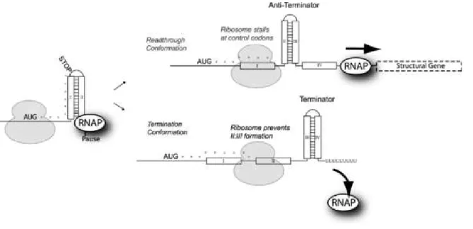
Fig. 1. Transcription terminates if the most recent portion of mRna is folded into a hairpin, when Rnap reaches a terminator Dna sequence.
2
Transcriptional Attenuation
Transcriptional attenuation prematurely interrupts a gene’s ongoing transcrip-tion, or that of an operon, when the cell does not actually need the corresponding proteins. E.coli ’s trp operon encodes enzymes for the biosynthesis of the amino acid tryptophan (Trp). Their production is attenuated if the bacterium’s envi-ronment provides sufficient amounts of tryptophan to feed on.
In this section, we first review the principles of gene expression in bacteria. Then, we introduce ribosome-mediated transcriptional attenuation, a regulatory mechanism used across bacterial species, and how specifically it functions at E.coli ’s tryptophan (trp) operon [13,36,37]. We omit certain aspects documented in the biological literature that do not enter our formal model presented in this paper, such as the role of transfer Rna in translation, or the redundancy of the genetic code.
Transcription copies information content from a Dna sequence into an mRna sequence. It is carried out by an enzyme called RNA polymerase. Rnap initiates its work by binding to a distinguished short Dna sequence which indicates the beginning of a gene (or operon), from where Rnap starts assembling an mRna molecule. In the following elongation phase Rnap advances stepwise over Dna, extending the growing mRna nucleotide by nucleotide, progressing at an av-erage rate of 50 nucleotides per second. Transcription terminates when Rnap encounters a terminator sequence on Dna, if an additional condition is then ful-filled. Figure1 illustrates this additional condition, that depends on a property of the mRna being transcribed. The linear mRna sequence can fold into stable secondary structures, which due to their shape are called hairpins. In order for transcription to terminate, while the Rnap encounters a terminator sequence on Dna, the most recent portion of the transcript must be folded into a hairpin. Translation reads out an mRna molecule into the corresponding sequence of amino acids. It initiates with the binding of a ribosome to the free end of an
Rule-based Modeling of Transcriptional Attenuation 5
Fig. 2.Leader region of the trp mRna. Adjacent pairs of the four segments S1
to S4fold into alternative hairpins. The anti-terminator hairpin S2·S3promotes
transcription of the operon, whereas the terminator S3· S4 aborts it.
mRna, the other end of which is still being elongated by an Rnap. The ribo-some advances along the mRna towards the Rnap in steps of codons, which are words of three mRna nucleotides. For each codon, the ribosome adds the corresponding amino acid to the growing sequence. These amino acid sequences later fold into three dimensional structures known as proteins. While the average rate of translation is 15 codons per second, each step of the ribosome is actually limited by the abundance of the currently required amino acid. The ribosome slows down on codons for which the corresponding amino acid is in short supply. Transcriptional attenuation subtly couples the termination of an ongoing round of transcription to the translation efficiency of the first part of the nascent mRna, where this latter is limited by a critical amino acid (tryptophan, for the trp operon). The so-called leader sequence consists of the operon’s first few dozen nucleotides. Attenuation boils down to a race between the Rnap transcribing the leader Dna, and the ribosome translating the leader mRna. In a nutshell, the attenuation race is as follows. If the amino acid of interest is abundant, the ribosome advances at its maximal speed, and the terminator hairpin forms. Tran-scription then aborts. Conversely if the critical amino acid is rare, the ribosome stalls early within the leader. The stalled ribosome inhibits the terminator hair-pin, hence the Rnap wins the race, and transcription continues into the operon’s protein coding regions.
Trp leader architecture. The leader’s architecture is fundamental to attenuation at E.coli ’s tryptophan operon. We distinguish four segments S1to S4within the
leader mRna, see Fig. 2. Each pair of adjacent segments folds into a hairpin, if neither of the required segments is masked by a ribosome. Three different secondary structures can occur within the leader mRna of the trp operon. They are named by their respective roles in attenuation. The pairing of S1 with S2
represents the pause hairpin, that between S2 and S3 is the anti-terminator
hairpin, and the terminator shown in Fig.1 is the pairing of S3 with S4.
Hairpin co-occurrence and mutual exclusion. Each leader segment can only par-ticipate in one hairpin at the same time. Most importantly, the anti-terminator prohibits the terminator hairpin by sequestering S3. Because both require S2,
the pause hairpin excludes the anti-terminator. On the other hand, the pause hairpin (S1· S2) and the terminator (S3· S4) can co-occur, since they do not
compete for a shared segment. With respect to our model, we need to mention that hairpin formation is fater than any other reaction in the system. It is also important to bear in mind that the segments become available one by one while Rnap transcribes the trp operon’s leader, and that the leader transcript pro-gressively forms hairpins whenever the ribosome’s position allows. Hence, the leader mRna never indeed remains unfolded, as simplifyingly shown in Fig.2. The role of hairpins. The impact of hairpins on transcription is significant, they determine pausing of the Rnap and termination of transcription. As opposed to this, mRna hairpins do not impair translation. A translating ribosome disrupts hairpins along its way, without significantly slowing down. We now detail on the pause and terminator hairpins at E.coli ’s trp operon.
Pause hairpin. After Rnap has transcribed the segments S1 and S2, it
re-mains stalled on a strong Dna pause site, while the mRna rapidly folds into the pause hairpin. This combination resembles the conditions for transcription termination, however, it is reversible: Rnap resumes transcriptions after a ri-bosome has arrived along the transcript and disrupted the pause hairpin. Let us consider the details of this initial configuration for the attenuation race in Fig.3 (left). Rnap is stalled on the pause site on Dna, more precisely on the nucleotide that we refer to as Dna0. It has so far transcribed the leader up to
and including its segments S1 and S2, that have folded into the pause hairpin.
The approaching ribosome disrupts the pause hairpin with its step onto the 7th
codon of the leader mRna, which is the first step from the initial conformation in Fig.3. The attenuation race now starts.
Terminator hairpin. The Dna leader of the trp operon contains a terminator sequence, just after the portion that encodes S4, see Fig.1. When Rnap arrives
here, the terminator mRna hairpin can form. The combination of terminator mRna hairpin and terminator Dna sequence aborts transcription. However if the anti-terminator is already present when S4 is completed - it can appear as
soon as S2 and S3 have been transcribed - the terminator is prevented. In this
case Rnap continues unhindered through the terminator sequence, and reaches the enzyme-coding region of the operon (the structural genes).
Trp codons within the leader mRNA. We have not yet mentioned the codons 10 and 11 of the leader mRna (see Fig. 2), the translation of which each requires one tryptophan molecule. These two control codons determine the outcome of attenuation race. They act as sensors for the tryptophan concentration, and determine the speed of the ribosome’s forward movement.
If tryptophan is in rare, the ribosome stalls on the control codons, hence its footprint does not advance far enough to mask the second segment. Soon later, the anti-terminator hairpin forms between S2 and S3, and transcription
continues into the structural genes. This is depicted as read-through configuration in Fig.3.
Conversely if tryptophan is abundant, the ribosome efficiently translates through the control codons. From the time point the ribosome has reached the
Rule-based Mo deling of T ranscriptional A tten uation 7
Fig. 3. Starting point and possible outcomes of the attenuation race at E.coli ’s trp operon. Initial conformation (left): Rnap is paused by the pause hairpin, awaiting to be released by the ribosome’s next step. Readthrough conformation: when tryptophan supply is low, the ribosome stalls on the control codons, the anti-terminator hairpin forms and transcription continues into the operon. Termination conformation: when tryptophan supply is high, the ribosome rapidly translates over the control codons. Before it unbinds from the mRna, the terminator hairpin forms and transcription aborts. Figure reproduced with permission from Elf and Ehrenberg (2005) [11].
13thcodon, and until it dissociates from the stop codon 15, the ribosome’s
foot-print masks S2, which prevents the anti-terminator [29]. The ribosome’s
unbind-ing delay from the stop codon is generally one second, which is a considerably long time scale, compared to all other reactions in the system. While S2remains
blocked by the ribosome, Rnap continues transcription, it completes S3 when
reaching the 36thDnanucleotide, and S
4 at the 47thDnanucleotide. The
ter-minator hairpin then forms and transcription aborts – this is the termination configuration.
Basal read-through due to premature ribosome release. A third possible out-come of the race is not covered by Fig.3. When tryptophan supply is high, the ribosome occasionally dissociates from the stop codon sooner than expected. In that case S3 can already have been transcribed, but S4 not yet. Hence S1, S2
and S3 are available at the same time. With equal probability, either the pause
hairpin or the anti-terminator forms, and in case of the latter, transcription con-tinues. This basal read-through of the operon has been experimentally observed for 10 − 15 % of initiated transcripts when tryptophan is abundant [18].
3
Rule Schemas for Chemical Reactions
In this section we first provide a formal and minimal rule-based language tai-lored to our needs (Sect. 3.1). We define chemical reactions, that operate on multisets of complex molecules with attributes such as Rnap · Dna(23). Herein, the infix operator · indicates a complex between Rnap that is bound within a Dna sequence, more precisely at the position 23 stated by the attribute value of the Dna nucleotide. Other attributes of molecules could be the compartment of a molecule, or information on its states, for instance folding or binding state. In Sect. 3.2, we present a language of rules schemas, that allows to define finite sets of chemical reactions in a compact manner. Rule schemas are like chemical reactions, except that attribute values are now extended to expressions with variables. All variables are universally quantified over finite sets, such that a rule schema defines a finite set of reactions. An example of a complex molecule is the term Rnap · Dna(x + 1) where x is a variable with values in {0, . . . , 50}. We introduce our language’s stochastic semantics in Sect.3.3.
As discussed in Sect. 3.4, more general ruled-based languages might have been used for our modeling study. The language in this paper is not intended as a contribution on its own, for the sake of its simplicity we however chose it for our presentation. Indeed, we relied on the software tool for another rule-based language to implement our models of Sect.4and5.
3.1 Chemical Reactions
In order to define the syntax of attributed molecules, we fix a possibly infinite set of attribute values C and a finite set N of molecule names. We assume that each molecule name N ∈ N has a fixed arity ar(N ) ≥ 0, which specifies its number of attributes.
Rule-based Modeling of Transcriptional Attenuation 9
Molecules M ∈ Mol ::= N(c1, . . . , cn) | M1· M2
Solutions S∈ Sol ::= M | S1, S2
Reactions S1→kS2
Table 1. Chemical reactions where N ∈ N , c1, . . . , cn ∈ C, ar(N ) = n and
k ∈ R+∪ {∞}.
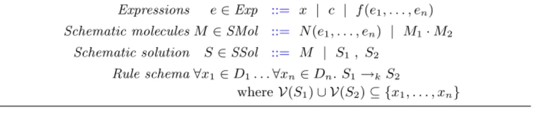
Expressions e∈ Exp ::= x | c | f (e1, . . . , en)
Schematic molecules M ∈ SMol ::= N(e1, . . . , en) | M1· M2
Schematic solution S∈ SSol ::= M | S1 , S2
Rule schema ∀x1∈ D1. . .∀xn∈ Dn. S1→kS2
where V(S1) ∪ V(S2) ⊆ {x1, . . . , xn}
Table 2. Rule schemas where x ∈ V, c ∈ C, f ∈ F, e1, . . . , en ∈ Exp, N ∈ N ,
ar(N ) = n, D1, . . ., Dn⊆ C are finite sets, and k ∈ R+∪ {∞}.
A molecule M , defined in Table1, is a complex of attributed molecules. We write M1· M2 for the complex of M1and M2. For instance, if Rnap, Dna ∈ N
and 47 ∈ C then Rnap · Dna(47) is a molecule complex consisting of an Rnap that is bound to the Dna nucleotide at position 47. A chemical solution S is a multiset of molecules.
A chemical reaction is a rule that rewrites a solution S1into a solution S2, it is
assigned a possibly infinite stochastic rate constant k ∈ R+∪ {∞}. For instance,
the following reaction states that an Rnap bound to the Dna nucleotide at position 23 may advance to the Dna nucleotide at position 24. The speed of this reaction is 50 sec−1:
Rnap· Dna(23) , Dna(24) →50 Dna(23) , Rnap · Dna(24)
In order to represent transcription, one would need many similar rules for the many other Dna nucleotides with different positions. This motivates the intro-duction of rule schemas, that allow to define such sets of chemical reactions in a compact manner.
3.2 Rule Schemas
In order to define rule schemas for chemical reactions, we introduce variables x for attribute values and expressions such as x + 1, in order to compute cor-responding attribute values. By universal quantification over a finite set, we generalize the above chemical reaction to the following rule schema:
∀x ∈ {1, . . . , 49}.
We thus need a set V of variables that are ranged over by x, and a finite set F of function symbols f ∈ F with arities ar(f ) ≥ 0. Furthermore, we assume an interpretation Jf K : Car(f ) → C for every f ∈ F. An expression e with values
in C is a term with the abstract syntax given in Table 2. In our modeling case studies, we will assume that symbol + ∈ F of arity two is interpreted as addition on natural numbers. We freely use infix syntax as usual, i.e. we write e1+ e2
instead of +(e1, e2). Given a variable assignment α : V → C, every expression
e ∈ Exp denotes an element JeKα∈ C that we define as follows:
JcKα= c JxKα= α(x) Jf (e1, . . . , en)Kα= Jf K(Je1Kα, . . . , JenKα)
A schematic molecule M is like a molecule, except we now allow for expressions in attribute positions rather than attribute values only. A schematic solution S ∈ SSol is a multiset of schematic molecules. As usual, we write V(S) for the set of variables that occur in molecules of S. A rule schema specifies the domains of variables occurring in the schematic solutions of the rule by universal quantification over finite sets.
For every variable assignment α : V → C that maps variables to values in their domain, we can instantiate the rule schema to finitely many reactions. A schematic molecule M is mapped to a molecule JM Kα∈ Mol. Similarly, schematic
solutions S ∈ SSol get instantiated to solutions JSKα∈ Sol:
JN (e1, . . . , en)Kα= N (Je1Kα, . . . , JenKα)
JM1· M2Kα= JM1Kα· JM2Kα
JS1, S2Kα= JS1Kα, JS2Kα
A rule schema is instantiated to a set of chemical reactions, by enumerating the chemical reactions for all variable assignments licensed by the quantifiers:
J∀x1∈ D1. . . ∀xn∈ Dn. S1→kS2K =
{JS1Kα→kJS2Kα| α : V → C, α(x1) ∈ D1, . . . , α(xn) ∈ Dn}
3.3 Stochastic Semantics and Simulation
For the sake of completeness, we recall the stochastic semantics of chemical reac-tions and how to use them for the stochastic semantics with Gillespie’s algorithm. This underlines that our biological modeling case studies are indeed expressed in a formal modeling language.
The semantics of a set of chemical reactions is a continuous time Markov chain (ctmc). Note that, for modeling convenience, we allow infinite rate constant ∞. Chemical reactions with infinite rates always have the highest priority and are executed immediately, that is without time delay. Such extended ctmcs with infinite rate constants can actually be converted to regular ctmcs by elimination of immediate transitions, while preserving sojourn time (i.e. how long the Markov chain stays in a given state) and probability transitions (that is, given a current state, the probability to make a transition to another given state)4.
Rule-based Modeling of Transcriptional Attenuation 11 L⊆ {1, . . . , n} ⊕i∈LMi≡ S S→kS′ ⊕n i=1Mi−→k L S ′, ⊕ i6∈LMi r=P {(L,k)|S−→k L S1≡S ′}k ¬∃L∃S ′′.S ∞ −→ L S ′′ S−→ Sr ′ n= ♯{L | S → S1≡ S′} m= ♯{L | S → S2} S−−−−−→ S∞(n/m) ′
Table 3.Stochastic semantics of chemical reactions with finite and infinite rate constants.
The states of the extended ctmcs are congruence classes [S]≡ of chemical
solutions S with respect to the least congruence relation ≡ that makes complex-ation and summcomplex-ation associative and commutative:
M1· M2≡ M2· M1 (M1· M2) · M3≡ M1· (M2· M3)
S1, S2≡ S2, S1 (S1, S2) , S3≡ S1, (S2, S3)
In Table3, we introduce transitions S −→k
L S
′ stating that S can be reduced to S′
by applying a chemical reaction with rate constant k ∈ R+∪{∞} to the subset of
molecules in S with positions in L. Positions are the indices in multisets such as M1, . . . , Mnthat we also write as ⊕ni=1Mi. We next introduce two transitions
– S −→ Sr ′, where r ∈ R+ sums up all rate constants of chemical reactions
reducing S to S′, as many times as they apply for some index set L, provided
that no immediate reaction can occur,
– S−−−→ S∞(r) ′ where the corresponding probability is r = n/m. The number of
occurrences of immediate reactions leading from S to a solution congruent to S′ is n, and the number of all occurrences of immediate reactions starting
from S is m.
Such transitions are invariant under structural congruence, i.e. for all S1≡ S1′
and S2 ≡ S2′ it holds that S1 r −→ S2 (resp. S1 ∞(r) −−−→ S2) if and only if S1′ r − → S′ 2 (resp. S′ 1 ∞(r) −−−→ S′
2). We can thus define [S]≡ r − → [S′] ≡ by S r − → S′and [S] ≡ ∞(r) −−−→ [S′] ≡ by S ∞(r)
−−−→ S′ as the transitions of the extended ctmc.
Gillespie’s algorithm for stochastic simulation takes as input a finite set of chemical reactions and a chemical solution S. If reactions with infinite rate con-stants are applicable, it computes n and m as defined above for each immediately reachable solution S′, and returns such an S′with probability n/m jointly with a
null time delay. Otherwise, it computes the overall rate of all possible transitions
R = P
{r|S−→r S1}r, returns with probability r/R a solution S1 with transition
S −→ Sr 1 jointly with a time delay drawn randomly from the exponential
distri-bution with rate r.
3.4 Language Design Choices and Related Rule-based Languages Models with rule schemas are more compact than if only simple reactions were used, thus easier to read. Attributed molecules and expressions that manipulate them were introduced, in the context of biological modeling languages, in [17]. Note that even if rule schemas could be defined solely by means of variables, function symbols allow a better control and precision of the collection of reactions that are generated. For example, without function symbols, we would need to resort to name sharing to represent Dna sequences5. Each Dna nucleotide would bear two parameters, one referring to its predecessor, the other to its successor. Given link names {ℓ0, . . . , ℓ50}, our previous rule (0) on page9 reads as
∀x, y, z ∈ {ℓ0, . . . , ℓ50}.
Rnap· Dna(x, y) , Dna(y, z) →50Dna(x, y) , Rnap · Dna(y, z) Then starting from a DNA sequence Dna(ℓ0, ℓ1), Dna(ℓ1, ℓ2), . . . , Dna(ℓ49, ℓ50),
this rule schema instantiates into more ground rules than needed. For exam-ple, the rule Rnap · Dna(ℓ1, ℓ10) , Dna(ℓ10, ℓ45) →50 Dna(ℓ1, ℓ10) , Rnap ·
Dna(ℓ10, ℓ45) is a meaningless instance of the above schema. Indeed, it is never applicable if the above DNA sequence is not modified as it is expected in a correct model.
All models written with our rule schemas can be compiled, by instantia-tion, to finite collections of simple and formally well-defined chemical reactions. Although reactions do not define a Turing-complete language [5], their expres-siveness is sufficient for our purposes. Furthermore, such collections of reactions are supported by standard tools for stochastic simulation such as Dizzy [27] or the rule-based language BioCham [6].
Alternative rule-based languages with higher expressiveness are Turing com-plete, e.g. the graph rewriting language Kappa [9], BioNetGen [16], and bigraphs [21]. Their pattern based graph rewriting rules resemble schemas, but their se-mantics is not based on instantiations to ground rules. They rather directly apply to arbitrary subgraphs satisfying the pattern. In contrast to our approach, such patterns may describe infinitely many reactions. Furthermore, stochastic sim-ulation is possible without inferring all those reactions on before hand. This generation process is uncritical in the present paper, since the overall number of reactions remains small, but is the bottleneck in other applications, where it grows exponentially [8,35]. Another promising language is LBS [24]. Its general purpose semantics allows for translations to different concrete semantics such as ODEs and ctmcs. LBS also features compact description of reactions with yet
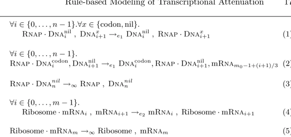
Rule-based Modeling of Transcriptional Attenuation 13 ∀i ∈{0,. . . ,n-1}.Rnap · Dnai, Dnai+1→e1Dnai, Rnap· Dnai+1 (1)
Rnap· Dnan→∞Rnap, Dnan (2)
∀i ∈{0,. . . ,m-1}.
Ribosome · mRnai, mRnai+1→e2 mRnai, Ribosome · mRnai+1 (3)
Ribosome · mRnam→∞Ribosome , mRnam (4)
Table 4. Rules for n transcription steps, in race with m translation steps.
another approach by means of parameterized modules, species expressions and “non-deterministic” species. These formal rule-based languages were designed and used so far to tackle protein-protein interactions that occur in cellular sig-naling such as metabolic pathways. In contrast to this, our rule-based model deals with a fine-grained mechanism of gene regulation.
4
Hyper-Sensitivity of Multi-Step Races
In this section we illustrate rule schemas for chemical reactions with a simple yet interesting example, borrowed from Elf and Ehrenberg (2005) [11]. Abstracting away from its detailed control by mRna hairpins, transcriptional attenuation boils down to a plain race between the two competing multi-step processes of transcription and translation. As intuition easily confirms, the probability that transcription wins the race decreases as the ribosome speeds up, and vice versa. We present two rule-based models for this multi-step race.
The basic model of Sect.4.1investigates the hyper-sensitivity of attenuation depending on the respective number of transcription versus translation steps (n vs m). Using Elf and Ehrenberg’s rate constants for transcription and transla-tion, we reproduce the results of Fig. 2 in [11].
In Sect.4.2we enrich our basic model by what we call concurrent elongation. An additional parameter m0 denotes the number of codons contained in the
initial solution, the remaining codons are dynamically spawn by the Rnap at simulation time. We show the impact of this additional level of concurrency, with respect to the attenuation race, through simulation.
4.1 Basic Model of Transcription and Translation
Elf and Ehrenberg demonstrated that the relative change in the probability that transcription wins the race can be much sharper, than the relative change in the ribosome’s speed. As our work confirms, this hyper-sensitivity of attenuation is determined by the number of transcription steps (n) versus translation steps (m). We give a basic rule-based model that allows to reproduce the results of Elf and Ehrenberg. As we believe, our framework is easier to understand and less prone
to error than the master equation approach, while compact and mathematically well-founded.
Model. The following initial solution describes the starting point of the multi-step race, where the Rnap and ribosome are bound to the first positions of Dna and mRna respectively:
Rnap· Dna0, ⊕ni=1Dnai , Ribosome · mRna0, ⊕mi=1mRnai
We use the following notational conventions. Molecule names are N = {Rnap, mRna, Dna, Ribosome}, attribute values C = N0, function symbols F = {+},
variables V = {i}, and value parameters n, m ∈ C. Because our model’s at-tributed molecules bear only few arguments, for the sake of presentation we slightly differ from the formal syntax introduced in Sect.3. We write attributes as indices for molecule names, instead of parenthesizing them, e.g. Dnai
in-stead of Dna(i). Moreover we write ⊕n
i=1Dnai instead of Dna(1), . . . , Dna(n).
Finally, we emphasize that each mRnai denotes one codon, which biologically
speaking is a sequence of three individual mRna nucleotides, that the ribosome reads out in one step.
Our model’s rule schemas are listed in Table4. Rule1 for the n steps of the transcribing Rnap from one Dna nucleotide to the next remains as in Sect.3.2, where it was the running example. The translation rule3 is analogous and re-flects the ribosome’s m steps over codons. The remaining rules2and4model the dissociation from the respectively last positions of Dna and mRna. Note that, bearing rate ∞, dissociation occurs without advance of the simulation clock. Hence it does not quantitatively affect our simulation results compared to the model of Elf and Ehrenberg, that does not include dissociation. In order to in-corporate the control conditions at the trp operon, we will refine the dissociation rules in Sect.5.
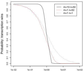
Simulation. The plot reporting our simulation results in Fig. 4 is organized as follows. The y-axis gives the probability that Rnap wins the race, on a scale between zero and one. It corresponds to the proportion of simulations in which Rnap dissociates before the ribosome does. The x-axis reports the translation rate on a logarithmic scale, that we vary from 0.01 to 100 codons per second in our simulations with the Kappa Factory [8].
The three models that each contribute one curve in the plot only differ in their numbers of translation (m) versus transcription (n) steps. We combined (m = 1 vs n = 1), (m = 1 vs n = 50), and (m = 10 vs n = 50).
Let us compare the sensitivity of these three models. When m = 1 and n = 1, the probability curve decreases gently, already showing some non-linearity. Increasing the number of transcription steps to n = 50 steepens the curve, i.e. increases the sensitivity. The transition becomes even sharper when the number of translation steps reaches higher values (m = 10, n = 50). Such values hold for systems where, unlike at E.coli ’s trp operon, attenuation is the sole control mechanism [19]. It is worthwhile pointing out that in this model each of the m
Rule-based Modeling of Transcriptional Attenuation 15
1e−02 1e−01 1e+00 1e+01 1e+02
0.0 0.1 0.2 0.3 0.4 0.5 0.6 0.7 0.8 0.9 1.0
Average rate e2′′ for m translation steps
Probability: transcription wins
m=10 n=50 m=1 n=50 m=1 n=1
Fig. 4. Probability that transcription wins in the basic model, as a function of the average translation rate e′
2, for different numbers of translation (m) versus
transcription (n) steps.
translation steps potentially slows down the ribosome’s advance, while at E.coli ’s trp operon, only 2 in 9 steps do.
Our rate constants are calculated as in [11], to ensure the outcomes of the three races are comparable. We keep the total time to perform the series of n transcription steps constant, such that 1/e′
1= 1 sec. Thus, the rate constant for
one individual transcription step out of n is e1= n · e′1. For one translation step
the rate constant is e2= m · e′2. Hereby e′2 is the average rate for m translation
steps, which varies logarithmically between 0.01 and 100.
As the next section will show, our model can smoothly be extended by ad-ditional concurrent issues, that are more difficult to handle within the master equation approach.
4.2 Concurrent Elongation of mRNA
In the basic model, the multi-step race was represented by a ribosome and an Rnapadvancing along two independent strands of mRna and Dna. Here we add what we call concurrent elongation to the multi-step race. The idea is to reflect that Rnap still elongates a transcript when the ribosome starts translating its older end. Translation can now become limited by the slower transcription: the ribosome can only translate those codons that have previously been produced by the Rnap. Our simulation results demonstrate that the outcome of the race depends on the length of the initially available mRna.
0 1
m
0-1
0,nil 1,nil 2,codon 3,nil ... 3(m+1-m0)-1,codon n-1,nil ...
RNAP
... Ribosome
last codon
transcribed here RNAP's target
Fig. 5.General initial solution for the concurrent elongation model, containing an mRna of length m0and a Dna of length n. The Dna is composed such that
upon simulation, every three steps of the Rnap one new codon is spawn; the final solution contains m codons.
Model. Compared to the basic model, we now explicitly elongate the previously available mRna in each transcription step. As Fig. 5 illustrates, a portion of the mRna is available to the ribosome from the beginning of the race. In the basic model the parameters n and m denoted the respective lengths of the Dna and mRna sequences for the attenuation race. Here the transcript dynamically grows from an initial length (for which we introduce the new parameter m0) to
its final length m.
We use two more function symbols for integer arithmetics than previously, F = {+, −, /}, attribute values C = N0∪ {codon, nil}, the previous molecule
names N = {Rnap, mRna, Dna, Ribosome}, and variables V = {i, x}. Dna molecules now come with a second attribute with values in {codon, nil}, noted as an upper index and with the following meaning. When Rnap leaves the ith nucleotide Dnacodon
i , it produces a new codon. As opposed to this, Dnanili
indicates that no new codon is spawn when Rnap passes from the ithnucleotide
to the next.
The choice of an appropriate initial solution is crucial to the proper function-ing of this model, because we want the polymerase to spawn one new codon every three Dna nucleotides. Assuming that Rnap is initially bound to Dna0 the
so-lution must be such that, for i mod 3 = 2, nucleotides are of the form Dnacodoni ,
and otherwise Dnanili . Correspondingly the first two nucleotides must be Dna nil 0
and Dnanil1 , followed by the nucleotide Dnacodon2 , and so forth respecting the
pattern nil, nil, codon. If only one codon is part of the initial solution (m0= 1)
we obtain:
Ribosome · mRna0,
Rnap· Dnanil0 , Dnanil1 , Dnacodon2 , Dnanil3 , Dnanil4 , Dnacodon5 , . . . , Dnaniln
Rule-based Modeling of Transcriptional Attenuation 17 ∀i ∈ {0, . . . , n − 1}.∀x ∈ {codon, nil}.
Rnap· Dnanili , Dnaxi+1→e1 Dnanili , Rnap· Dnaxi+1 (1)
∀i ∈ {0, . . . , n − 1}.
Rnap· Dnacodoni , Dnanili+1→e1 Dnacodoni , Rnap· Dnanili+1,mRnam
0−1+(i+1)/3 (2)
Rnap· Dnaniln →∞Rnap, Dnaniln (3)
∀i ∈ {0, . . . , m − 1}.
Ribosome · mRnai, mRnai+1→e2 mRnai, Ribosome · mRnai+1 (4)
Ribosome · mRnam→∞Ribosome , mRnam (5)
Table 5.Rules for concurrent elongation (n steps), where the transcribing Rnap adds one new codon to the solution every three Dna nucleotides.
For the sake of simplicity we do not show the Dna position corresponding to mRnam. When m0= m + 1, the initial solution reduces to that of Sect.4.1:
Ribosome · mRna0, ⊕mi=1mRnai,
Rnap· Dnanil0 , Dnanil1 , Dnacodon2 , Dnanil 3 , Dna nil 4 , Dna codon 5 , . . . , Dna nil n
Figure 5 illustrates the general case. In addition to the constraint on Dna nucleotide alternation, we assume that the initial solution contains m0 codons,
that the rule set will lead to the dynamic supply of additional m − m0 codons,
such that the final solution shall contain m+1 codons (allowing for m translation steps), and that 1 ≤ m0 ≤ m < 13n. The ribosome’s target codon mRnam
corresponds to the Dna position 3 · (m − m0+ 1) − 1. Beyond this, we assume
that Rnap eventually reaches its own target, the nth position of Dna, without
injecting additional codons to the solution.
Table5lists our rule schemas. The rule1for one step of the Rnap, in which no codon is produced, resembles rule 1of Sect.4.1. It applies when leaving nu-cleotides of the form Dnanili , whether or not the step leaving the next nucleotide
yields a codon. Hence the quantification over x ∈ {codon, nil} for Dnaxi+1.
The complementary rule 2 injects a new codon into the solution when the Rnapleaves a nucleotide of the form Dnacodoni . The new codon’s index is cal-culated from the current Dna position i and the initially available number of codons by the arithmetic expression m0− 1 + (i + 1)/3. By doing so, we ensure
that Dna2 yields mRnam0, Dna5 yields mRnam0+1, etc. up to the ribosome’s
target mRnam.
The rule for the Rnap’s dissociation from Dna (3) only marginally differs from that of the previous subsection (in that the nucleotide bears the second attribute nil), and the ribosome advance and release rules (4and5) remain just the same.
1e-02 1e-01 1e+00 1e+01 1e+02 0 .0 0 .2 0 .4 0 .6 0 .8 1 .0
Average rate e2′ for m translation steps
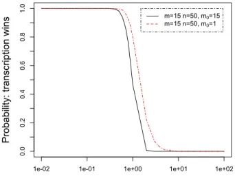
Pro b a b ili ty: t ra n scri p ti o n w in s m=15 n=50, m0=15 m=15 n=50, m0=1
Fig. 6.Probability that transcription wins in the concurrent elongation model, as a function of the average translation rate e′
2, for different numbers of initially
available codons (m0 = 15 vs m0 = 1), but the same number of transcription
steps (n = 50) and translation steps (m = 15).
Simulation. We simulated our concurrent elongation model within the Kappa factory with several combinations of m0, m and n. Figure6shows the outcome
of the race distinguishing whether only one codon is initially present (m0= 1),
or all (m0= m), for the same number of translation (m = 15) and transcription
steps (n = 50).
When all codons are contained in the initial solution (m0 = 15), the
sim-ulation results reduce to those of the basic model, whereas for m0 = 1, the
simulation curve shifts to the right, meaning that the probability that transcrip-tion wins the race increases. Indeed for each translatranscrip-tion step, the ribosome’s advance is potentially limited by the polymerase, that needs to add a further codon to the mRna. Hence, even if translation is efficient, the polymerase wins more often than for m0 = 15. In our simulations we observed a lesser shift for
m0= 10, not included in the plot.
Our simulations underline that the outcome of the multi-step race is param-eterized not only by the n transcription steps and the m translation steps, but also by the number m0of initially available codons. This last parameter only
ap-pears when the model integrates concurrent elongation. We can now summarize our analysis of the multi-step race parameterized by m, n and m0, in terms of
the shape of the curve that represents the probability that the polymerase wins the race:
Rule-based Modeling of Transcriptional Attenuation 19 – As pointed out by Elf and Ehrenberg [11], the ratio of m to n determines the curve’s slope. They are the key parameters of the hyper-sensitivity of ribosome-dependent transcriptional attenuation.
– Varying m0shifts the curve. The polymerase’s chance to win increases with
m0, when m and n remain fixed, because m0 constrains the ribosome’s
ad-vance along mRna. As we observed, the shift increases with the difference between m and m0.
Incorporating concurrent elongation into our model was facilitated by our rule-based approach with arithmetic. It would have been more difficult with probability functions. In a model that includes concurrent elongation, the posi-tions of the ribosome and the Rnap are not independent. The advance of the former is limited by that of the latter. This point was not considered in [11].
5
Modeling Transcriptional Attenuation
This section presents our rule-based model of ribosome-mediated transcriptional attenuation at E.coli ’s tryptophan operon. It refines our basic model of Sect.4.1
in several points. The messenger Rna’s representation dynamically grows while we simulate Rnap’s advance, similarly as in the concurrent elongation model. But whereas in Sect. 4.2, we only used individual codons as building blocks of the transcript, the attenuation model also features mRna segments as a whole. Explicit representations of S1, S2, S3, and S4allow us to smoothly cover the
dy-namics of secondary structure formation, and incorporate the regulatory impact of hairpins on transcription. We make one notable exception to our all-in-one representation of mRna segments. Regarding S1, we switch between two
dif-ferent abstraction levels depending on the context, either representing it as a whole, or enumerating its codon sequence (⊕14
i=10mRnai).
After introducing our attenuation model, we present simulation results in Sect.5.2, and then explain the quantitative differences between our results and those of Elf and Ehrenberg [11] in Sect.5.3.
5.1 Rule Schemas
Table 6 provides the rule schemas of our detailed attenuation model. The no-tational conventions are based on those of our basic model of Sect. 4.1. We use molecule names N = {Rnap, mRna, Dna, Ribosome, S}, where Dna nu-cleotides are unary, attribute values C = N0 ∪ {fr, bl, hp}, function symbols
F = {+}, and variables V = {i, n, m, t, x}. Molecules with two attributes Sxi
represent segments of the mRna leader. Their lower index i ∈ {1, 2, 3, 4} de-notes the segment’s number, and the upper index x the segment’s state which is among:
– free (fr): available for hairpin formation,
– blocked (bl): masked by the ribosome’s footprint,
– hairpin (hp): complexed into a hairpin with a neighboring segment. For instance, Shp1 · Shp2 denotes the pause hairpin.
The initial solution for our simulations reflects the starting configuration for the attenuation race, depicted in Fig.3on page7:
Rnap· Dna0, ⊕50i=1Dnai,
Ribosome · mRna6, mRna7, mRna8, mRna9,
Shp1 · Shp2 , mRna15
(0) Rnaphas transcribed the leader up to and including S1and S2, that are paired into the pause hairpin, and is paused on the zero-th Dna nucleotide, that is followed by a sequence of 50. The ribosome has initiated translation and is located on the 6th codon of the transcript leader. We explicitly render the codons 6 to 9, which precede the segment S1, and the stop codon 15, that is located
between the segments S1 and S2. In contrast, we do not render the codons
preceding 6, since they do not matter to the attenuation race, and for the same reason we will not provide rules for the initiation of transcription and translation. Hairpin formation is covered by rule schema1, be it for the pause hairpin, the anti-terminator or the terminator. Because hairpin formation occurs on a much faster time scale than any other reaction, we approximate it with an infinite rate constant.
Translation rules (schemas 2 to 7 in Table 6). Rule schema 2 covers the bulk of translation steps, that do not have side effects, nor depend on tryptophan availability or other side conditions. It bears the reaction rate constant e2 =
15s−1, i.e. the ribosome makes 15 steps over mRna per second, in average. Rule
schema 3 deals with the ribosome’s step over the tryptophan codons within the leader, i.e. the control codons 10 and 11, where the distinct elongation rate constant e3 holds. We will vary e3 within ]0, 15]s−1 in our simulations, while e2
remains fixed.
Starting from our initial solution (the above equation0) the next important event is melting the pause loop Shp1 · Shp2 , as the ribosome steps from mRna6
to mRna7. Two points are worthwhile noting in rule 4’s right part. First,
ob-viously since the pause loop is melt, S2’s state becomes free - and one could
similarly expect a stage change at S1. But second and more importantly, instead
of switching S1’s state, we pass from the abstraction of the segment as a whole,
to the enumeration of the codons ⊕14
i=10mRnai that make it up. The sequence
enumeration remains part of the solution as long as the ribosome’s footprint par-tially covers the first segment, i.e. until it dissociates from the stop codon. This implicitly sequesters S1 from hairpin formation – which would instantaneously
occur through schema1if both S1 and S2 were around and in their free state.
For the ribosome’s step from mRna12 to mRna13, we introduce two rules
with distinct preconditions. The common result of both is to reflect that the second segment gets masked by the ribosome’s footprint, i.e. both rules produce Sbl2. When S2 is initially free, rule 5 applies. Otherwise, S2 is paired into the anti-terminator hairpin, and rule 6 handles its melting through the ribosome’s advance. When the ribosome dissociates from the stop codon (rule 7), S1
Rule-based Mo deling of T ranscriptional A tten uation 21 ∀i ∈ {1, 2, 3}.Sfri , Sfri+1→∞Shpi · S hp i+1 (1)
∀m ∈ {7, 8, 9, 13, 14}.Ribosome · mRnam, mRnam+1→e2 mRnam, Ribosome · mRnam+1 (2) ∀t ∈ {10, 11}.Ribosome · mRnat, mRnat+1→e3 mRnat, Ribosome · mRnat+1 (3)
Ribosome · mRna6, mRna7, Shp1 · S hp
2 →e2 mRna6, Ribosome · mRna7, ⊕ 14
i=10mRnai, Sfr2 (4) Ribosome · mRna12, mRna13, Sfr2 →e2 mRna12, Ribosome · mRna13, S
bl
2 (5)
Ribosome · mRna12, mRna13, Shp2 · S hp
3 →e2 mRna12, Ribosome · mRna13, S bl
2 , Sfr3 (6) Ribosome · mRna15, ⊕14i=10mRnai, Sbl2 →d Ribosome , mRna15, Sfr1 , Sfr2 (7) ∀n ∈ {1, . . . , 49} \ {35, 46, 47}.Rnap · Dnan, Dnan+1→e1 Dnan, Rnap· Dnan+1 (8)
∀x ∈ {fr, bl}.Rnap · Dna0, Dna1, Sx2 →e1 Dna0, Rnap· Dna1, S x
2 (9)
Rnap· Dna35, Dna36→e1 Dna35, Rnap· Dna36, Sfr3 (10) Rnap· Dna46, Dna47→e1 Dna46, Rnap· Dna47, S
fr
4 (11)
Rnap· Dna47, Shp3 · S hp
4 →e1 Dna47, Rnap , S hp 3 · S
hp
4 (12)
Rnap· Dna47, Dna48, Shp2 · S hp
3 →e1 Dna47, Rnap· Dna48, S hp 2 · S
hp
3 (13)
Transcription rules. Rules 8 to 13 in Table 6 represent transcription. Rule schema 8 represents one step of Rnap in the simplest possible fashion, that was already discussed in Sect.4.1with the rate constant e1 = 50s−1. It applies
to all Dna positions from 0 to 50 with a few exceptions that we discuss in the order they are applied, starting from our initial solution.
Transcription resumes at position Dna0 (rule schema 9) after the pause
hairpin has been disrupted. This is witnessed by S2being either free or blocked.
Note that it would have been simpler to check the absence of the pause hairpin, but such negative tests are neither supported by the language used in this paper, nor by most current rule-based frameworks and tools, a notable exception to a certain extent is offered by [16].
The remaining rules deal with the creation of new mRna segments, and (anti)termination of transcription. When Rnap steps over to Dna36, the Rna
segment S3 is injected into the solution (reaction 10). S4 follows at Dna47
(re-action 11). Transcription terminates on Dna47 provided there is a terminator
hairpin, see Shp3 · Shp4 in reaction12. If conversely the anti-terminator is present transcription proceeds to Dna48 (rule 13) and continues transcription into the
operon.
Summary: global control by n-ary rules. Finally we summarize our use of n-ary rules, that separates into three categories. Such n-ary rules can not be rendered in an intelligible fashion within object-centric approaches limited to binary in-teractions, namely π-calculus based modeling languages.
In the first category, we check whether the current solution fulfills a certain prerequisite, e.g. contains a certain molecule, or a certain molecule in a specific state. The rules for abortion versus continuation of transcription (rules12 and
13) depend on which hairpin is around, terminator or anti-terminator. Other prerequisites we check are unfortunately less intuitive: sometimes one would prefer to impose negative conditions on rule application, which however is neither supported by our language, nor most other current rule-based frameworks. For instance, rule9resumes transcription if the pause hairpin is absent, which is the case if S2’s state is free or blocked.
The second category are reactions that actually occur between two molecules, but entail the modification of a third. Examples are the rules for blocking S2
as the ribosome proceeds to mRna13: rule5blocks S2, rule6 disrupts the
anti-terminator hairpin at the same time, such that the states of both S2 and S3
change. The third category is the abstraction level switching for mRna segments, that is assembling the first segment from the codons 10 to 14 in rule 7, versus splitting it in rule4.
5.2 Simulation
Figure 7 plots the relative transcription frequency (y-axis) against the rate of trp-codon translation e3 (x-axis). For each value of e3 from 0 to 15 s−1 in steps
Rule-based Modeling of Transcriptional Attenuation 23 0 5 10 15 0 .0 0 .1 0 .2 0 .3 0 .4 0 .5 0 .6 0 .7 0 .8 0 .9 1 .0
Rate e3 of trp-codon translation(s−1)
R e la ti ve f re q u e n cy o f tra n scri p ti o n ribosome release ribosome stalling total
Fig. 7. Relative frequency of continued transcription as a function of the trp-codon translation rate. We distinguishing between anti-terminator formation during ribosome stalling, and after release of the ribosome from the stop codon.
different pathways lead to the anti-terminator, each of them corresponds to a distinct curve, and a third curve sums up.
The curve ribosome stalling corresponds to anti-terminator formation while the ribosome remains stalled on the control codons. This predominates when trp-codon translation is slow, becomes rarer as the translation efficiency increases, and drops below 1% when e3≥ 9s−1.
In a second pathway, the anti-terminator hairpin forms after the ribosome has released from the stop codon 15. This represents the basal read-through level of the trp operon (see page 8). The corresponding curve ribosome release in our simulation plot starts from zero, steadily increases with the rate of trp-codon translation, reaches its maximal level around 4.5% at a rate of trp-trp-codon translation of 4 s−1, and remains stable henceforth.
Our results shown in Fig.7qualitatively confirm those of Elf and Ehrenberg [11]. However, even if the curves have the same shape, the asymptotic decrease of ribosome stalling toward 0 is less sharp in our case. While in their work the curves for ribosome release and ribosome stalling cross at a rate of 6s−1, in ours
they already do so at 5s−1. Moreover our experiments predict a rate of basal
transcription of slightly under 5% when trp-codon translation is efficient, where Elf and Ehrenberg predict 8%.
S1⋄S2 OFF S1,S2, S3⋄S4 S1,S2, S3 [13,15] S1,S2 S1,S2⋄S3,S4 anti-termination Ribosome stalling S1,S2⋄S3 [7,12] S1,S2 OUTCOME [47] [36,46] [0,35] Ribosome RNAP bl fr bl bl hp hp hp hp bl bl bl fr hp hp bl fr bl bl hp hp S1,S2⋄S3 Shp hp1⋄S2, S3fr fr hp hp 50% 50% 100% Sfr1,S2hp hp⋄S3,S4fr Shp hp1⋄S2, S3hp hp⋄S4 termination anti-termination Ribosome release A B
Table 7. Transitions between configurations of the trp leader that our model yields, depending on the relative positions of the ribosome versus Rnap. We list the first segment in its blocked state for the sake of presentation, when the solution indeed enumerates its sequence.
5.3 Discussion
We believe that the differences between our quantitative results and those of [11] are due to the greater level of detail rendered by our model. Elf and Ehrenberg reduce attenuation to a race between the ribosome and the polymerase, but their model does not make hairpins explicit. Instead, they infer transcription probabilities from the relative positions of both the Rnap and the ribosome. As opposed to this, our model explicitly renders hairpins.
Table7 summarizes how the configuration of the system evolves, assuming simulations start from our initial solution (equation 0), and the ribosome has disrupted the pause hairpin. For each relative position of the ribosome on mRna (columns) and the Rnap on Dna (rows), the table states which segments have been transcribed so far, and which hairpins have formed. Arrows between the table’s cells corresponds to possible transitions of our solution. We distinguish the following positions of interest for the Rnap on Dna:
• between DNA nucleotide 0 and 35: only segments S1 and S2 are
con-tained in the initial solution,
• between 36 and 46: Rnap has completed segment S3,
• on position 47: Rnap has injected S4to the solution.
The ribosome’s positions of interest on the mRna leader are:
• between codon 7 and 12: the ribosome’s footprint has not yet reached S2;
• between codon 13 and 15: the ribosome’s footprint masks S2 until
disso-ciation from the mRna.
• off: the ribosome has dissociated from the transcript, making segment S2
Rule-based Modeling of Transcriptional Attenuation 25 Elf and Ehrenberg distinguish two cases of anti-termination (reproduced in our simulations in Fig. 7): termination during ribosome stalling and anti-termination after ribosome release.
Stochastic trajectories leading to ribosome stalling descend our table’s col-umn [7, 12]. The ribosome then remains between the codons 7 and 12, most likely stalling on the control (trp) codons within the first segment. After the poly-merase has transcribed segment S3, the anti-terminator hairpin S2· S3 forms.
This henceforth excludes the terminator hairpin, and transcription continues into the structural genes. We believe that our model and that of Elf and Ehrenberg show the same behavior for this first pathway.
We identified the following key difference between the models regarding the second pathway to anti-termination. Elf and Ehrenberg assume that the proba-bility of anti-termination after ribosome release is half the probaproba-bility of reaching the configuration (Rnap ∈ [36, 46], ribosome OFF). The corresponding cell is highlighted in light gray in Table 7. It is important to note that we separate it into two sub-cells A and B. We refine Elf and Ehrenberg’s assumption as follows: stochastic trajectories leading to anti-termination after ribosome release pass through the sub-cell B, but never through the sub-cell A.
Careful consideration of the table explains our refinement. The highlighted cell can be reached from either its top or left neighbor. Coming from the left neighbor (Rnap ∈ [36, 46], ribosome ∈ [13, 15]), it is equally likely to reach sub-cell A that entails termination, as to reach B that entails anti-termination. However, coming from the top neighbor (Rnap ∈ [0, 35], ribosome OFF) makes a difference. Because the ribosome has unbound the mRna before segment S3was
completed, the pause hairpin Shp1 · S hp
2 is already part of the solution. Hence the
anti-terminator does not appear once S3is completed. Thus, descending the
col-umn ribosome off, the system always reaches configuration A, and transcription always terminates.
Based on our detailed model, and contradicting Elf and Ehrenberg, we claim that the state (Rnap ∈ [36, 46], ribosome off) does not lead with equal probabil-ities to anti-termination by ribosome release versus termination. The downward transitions into sub-cell A, that contains the pause hairpin Shp1 · Shp2 and hence excludes the anti-terminator, increase the termination probability6. This line of reasoning agrees with experimental knowledge on the impact of early ribosome release [29], and may explain why our experiments predict anti-termination less often than Elf and Ehrenberg’s.
6
Conclusion
We have shown that rule-based modeling provides concise and elegant models for the fine-grained mechanism of transcriptional attenuation, a problem left open by previous work on discrete event modeling of the tryptophan operon [32]. The
6 Another effect is due to the anti-terminator hairpin melting as the ribosome moves
on to mRna13 that is included in our model, which lowers the ribosome stalling
core ingredients for our model are rule schemas and n-ary chemical reactions. The importance of n-ary reactions renders representations of this case of ge-netic regulation in object-centered languages such as the stochastic pi-calculus [22,25,28] inappropriate, in practice. We used the Kappa factory for stochastic simulation [8], which provided us convenient analysis tools.
In our model we identified positions of individual nucleotides and codons within Dna and Rna sequences by numbers, abstracted over by variables, and addressed successors by simple arithmetic. This technique has its limitations when polymers become more complex than simple lists. Alternatively, we could assign names to molecular domains, and memorise those names in attribute values of adjacent molecules, similarly to Kappa. As shown in Sect.3.4, the cost for such an alternative is that meaningless instances of rule schemas may be generated.
In future work, we plan to compute the exact probability that the ribosome dissociates before the segment S3is formed. This corresponds to the additional
pathway that is not rendered by the model proposed by Elf and Ehrenberg (2005) [11]. This would formally prove what we conjectured to be the source of the quantitative difference between the two models. We can indeed compute such a probability because there are finitely many pathways and all pathways are terminating (i.e. the system always reaches a configuration in which no rule is applicable). In other words, one can exhaustively unfold the underlying ctmc and thus compute the probability associated to each pathway (i.e. each branch of the ctmc).
Acknowledgements. The Master’s project with Valerio Passini at the Microsoft Research - University of Trento Center for Computational and Systems Biology sharpened our view of the system from a biological perspective and lead us to a rule-based approach. The previous Master’s project of Gil Payet (co-supervised with Denys Duchier) had confronted us with the limitations of object-based ap-proaches to the representation of the complex dependencies of transcriptional attenuation. We thank Maude Pupin, who was the first to point us at the intri-cate regulatory mechanisms at E.coli ’s tryptophan operon, and Joachim Niehren for his valuable coaching. Plectix BioSystems kindly made the Kappa Factory available to us, and gave us useful support while we carried out the experi-ments reported in this paper. Finally, we thank the CNRS for a sabbatical to C´edric Lhoussaine, and the Agence Nationale de Recherche for funding this work through a Jeunes Chercheurs grant (ANR BioSpace, 2009-2011).
References
1. Adam Arkin, John Ross, and Harley H. McAdams. Stochastic kinetic analysis of developmental pathway bifurcation in phage λ-infected Escherichia coli cells.
Genetics, 149:1633–1648, 1998.
2. Franz Baader and Tobias Nipkow. Term rewriting and all that. Cambridge Uni-versity Press, New York, NY, USA, 1998.
Rule-based Modeling of Transcriptional Attenuation 27 3. Matjaz Barboric and B. Matija Peterlin. A new paradigm in eukaryotic biology: HIV Tat and the control of transcriptional elongation. PLoS Biology, 3(2):0200– 02003, 2005.
4. Chase L. Beisel and Christina D. Smolke. Design principles for riboswitch function.
PLoS Computational Biology, 5(4):e1000363, 04 2009.
5. Luca Cardelli and Gianluigi Zavattaro. On the computational power of biochem-istry. In Proceedings of the 3rd international conference on Algebraic Biology, pages 65–80, Berlin, Heidelberg, 2008. Springer-Verlag.
6. Nathalie Chabrier-Rivier, Francois Fages, and Sylvain Soliman. The biochemical abstract machine BioCham. In Proceedings of CMSB 2004, volume 3082 of Lecture
Notes in Bioinformatics, pages 172–191, 2005.
7. Federica Ciocchetta and Jane Hillston. Bio-PEPA: a framework for modelling and analysis of biological systems. Theoretical Computer Science, 2008. To appear. 8. Vincent Danos, Jerome Feret, Walter Fontana, and Jean Krivine. Scalable
sim-ulation of cellular signaling networks. In 5th Asian Symposium on Programming
Languages and Systems, volume 4807 of Lecture Notes in Computer Science, pages
139–157, 2007.
9. Vincent Danos, J´erˆome Feret, Walter Fontana, Russell Harmer, and Jean Krivine. Rule-based modelling of cellular signalling. In 18th International Conference on
Concurrency Theory, volume 4703 of Lecture Notes in Computer Science, pages
17–41, 2007.
10. L. Dematt´e, C. Priami, and A. Romanel. The beta workbench: A tool to study the dynamics of biological systems. Briefings in Bioinformatics, 9(5):437–449, 2008. 11. Johan Elf and Mans Ehrenberg. What makes ribosome-mediated trascriptional
attenuation sensitive to amino acid limitation? PLoS Computational Biology,
1(1):14–23, 2005.
12. Daniel T. Gillespie. A general method for numerically simulating the stochastic time evolution of coupled chemical reactions. Journal of Computational Physics, 22:403–434, 1976.
13. Paul Gollnick. Trp operon and attenuation. In William J. Lennarz and M. Daniel Lane, editors, Encyclopedia of Biological Chemistry, pages 267 – 271. Elsevier, New York, 2004.
14. Paul Gollnick, Paul Babitzke, Alfred Antson, and Charles Yanofsky. Complexity in regulation of tryptophan biosynthesis in Bacillus subtilis. Annual Review of
Genetics, 39(1):47–68, 2005.
15. A Gutierrez-Preciado, R.A. Jensen, C. Yanofsky, and E. Merino. New insights into regulation of the tryptophan biosynthetic operon in Gram-positive bacteria.
Trends in Genetics, 21(8):432–436, 2005.
16. Michael L. Blinov James R. Faeder and William S. Hlavacek. Systems Biology, volume 500 of Methods in Molecular Biology, chapter Rule-Based Modeling of Bio-chemical Systems with BioNetGen, pages 1–55. Humana Press, 2009.
17. Mathias John, C´edric Lhoussaine, Joachim Niehren, and Adelinde M. Uhrmacher. The attributed pi-calculus with priorities. Transactions on Computational Systems
Biology, 2009. To appear.
18. Y Nakamura JR Roesser and C. Yanofsky. Regulation of basal level expression of the tryptophan operon of Escherichia coli. J Biol Chem, 264(21):12284–8, 1989. 19. T Kasai. Regulation of the expression of the histidine operon in Salmonella
ty-phimurium. Nature, 249:523–527, 1974.
20. Kouacou Vincent Konan and Charles Yanofsky. Role of ribosome release in regu-lation of tna operon expression in Escherichia coli. J. Bacteriol., 181:1530–1536, 1999.