HAL Id: hal-01515951
https://hal.inria.fr/hal-01515951
Submitted on 28 Apr 2017
HAL is a multi-disciplinary open access
archive for the deposit and dissemination of
sci-entific research documents, whether they are
pub-lished or not. The documents may come from
teaching and research institutions in France or
abroad, or from public or private research centers.
L’archive ouverte pluridisciplinaire HAL, est
destinée au dépôt et à la diffusion de documents
scientifiques de niveau recherche, publiés ou non,
émanant des établissements d’enseignement et de
recherche français ou étrangers, des laboratoires
publics ou privés.
A multi-resolution approach to common fate-based
audio separation
Fatemeh Pishdadian, Bryan Pardo, Antoine Liutkus
To cite this version:
Fatemeh Pishdadian, Bryan Pardo, Antoine Liutkus. A multi-resolution approach to common
fate-based audio separation. 42nd International Conference on Acoustics, Speech and Signal Processing
(ICASSP), Mar 2017, New Orleans, United States. �hal-01515951�
A MULTI-RESOLUTION APPROACH TO COMMON FATE-BASED AUDIO SEPARATION
Fatemeh Pishdadian, Bryan Pardo
⇤Northwestern University, USA
{fpishdadian@u., pardo@}northwestern.edu
Antoine Liutkus
Inria, speech processing team, France
[email protected]
ABSTRACT
We propose the Multi-resolution Common Fate Transform (MCFT), a signal representation that increases the separabil-ity of audio sources with significant energy overlap in the time-frequency domain. The MCFT combines the desirable features of two existing representations: the invertibility of the recently proposed Common Fate Transform (CFT) and the multi-resolution property of the cortical stage output of an au-ditory model. We compare the utility of the MCFT to the CFT by measuring the quality of source separation performed via ideal binary masking using each representation. Experiments on harmonic sounds with overlapping fundamental frequen-cies and different spectro-temporal modulation patterns show that ideal masks based on the MCFT yield better separation than those based on the CFT.
Index Terms— Audio source separation, Multi-resolution Common Fate Transform,
1. INTRODUCTION
Audio source separation is the process of estimating n source signals given m mixtures. It facilitates many applications, such as automatic speaker recognition in a multi-speaker sce-nario [1, 2], musical instrument recognition in polyphonic au-dio [3], music remixing [4], music transcription [5], and up-mixing of stereo recordings to surround sound [6, 7].
Many source separation algorithms share a weakness in handling the time-frequency overlap between sources. This weakness is caused or exacerbated by their use of a time-frequency representation, typically the short-time Fourier transform (STFT), for the audio mixture. For example, the Degenerate Un-mixing and Estimation Technique (DUET) [8, 9] clusters time-frequency bins based on attenuation and delay relationships between STFTs of the two channels. If multiple sources have energy in the same time-frequency bin, the performance of DUET degrades dramatically, due to the inaccurate attenuation and delay estimates. Kernel Additive Modeling (KAM) [10, 11] uses local proximity of points belonging to a single-source. While the formulation of KAM does not make any restricting assumptions about the
⇤Thanks to support from National Science Foundation Grant 1420971.
audio representation, the published work uses proximity mea-sures defined in the time-frequency domain. This can result in distortion if multiple sources share a time-frequency bin. Non-negative Matrix Factorization (NMF) [12] and Proba-bilistic Latent Component Analysis (PLCA) [13] are popular spectral decomposition-based source separation methods ap-plied to the magnitude spectrogram. The performance of both degrades as overlap in the time-frequency domain increases.
Overlapping energy may be attenuated in better represen-tations. According to the common fate principle [14], spectral components moving together are more likely to be grouped into a single sound stream. A representation that makes com-mon fate explicit (e.g. as one of the dimensions) would facil-itate separation, since the sources would better form separate clusters, even when overlapping in time and frequency.
There has been some recent work in the development of richer representations to facilitate separation of sounds with significant time-frequency energy overlap. St¨oter et al. [15] proposed a new audio representation, named the Common Fate Transform (CFT). This 4-dimensional representation is computed from the complex STFT of an audio signal by first dividing it into a grid of overlapping patches (2D window-ing) and then analyzing each patch by the 2D Fourier trans-form. The CFT was shown to be promising for the separation of sources with the same pitch (unison) and different mod-ulation. However, they use a fixed-size patch for the whole STFT. This limits the spatial frequency resolution, affecting the separation of streams with close modulation patterns.
The auditory model proposed by Chi et al. [16] em-ulates important aspects of the cochlear and cortical pro-cessing stages in the auditory system. It uses a bank of 2-dimensional, multi-resolution filters to capture and rep-resent spectro-temporal modulation. This approach avoids the fixed-size windowing issue. Unfortunately, creation of the representation involves non-linear operations and remov-ing phase information. This makes perfect invertibility to the time domain impossible. Thus, using this representation for source separation (e.g. Krishnan et al. [17]) requires building masks in the time-frequency domain, where it is possible to reconstruct the time-domain signal. However, masking in time-frequency eliminates much of the benefit of explicitly representing spectro-temporal modulation, since time-frequency overlap between sources remains a problem.
Here, we propose the Multi-resolution Common Fate Transform (MCFT), which combines the invertibility of the CFT with the multi-resolution property of Chi’s auditory-model output. We compare the efficacy of the CFT and the MCFT for source separation on mixtures with considerable time-frequency-domain overlap (e.g. unison mixtures of mu-sic instruments with different modulation patterns).
2. PROPOSED REPRESENTATION
We now give brief overviews of the Common Fate Trans-form [15] and Chi’s auditory model [16]. We then pro-pose the Multi-resolution Common Fate Transform (MCFT), which combines the invertibility of the CFT with the multi-resolution property of Chi’s auditory-model output.
2.1. Common Fate Transform
Let x(t) denote a single channel time-domain audio sig-nal and X(!, ⌧) = |X(!, ⌧)|ej\X(!,⌧) its complex time-frequency-domain representation. Here, ! is frequency, ⌧ time-frame, |.| is the magnitude operator, and \(.) is the phase operator. In the original version of CFT [15], X(!, ⌧) is assumed to be the STFT of a signal, computed by window-ing the time-domain signal and takwindow-ing the discrete Fourier transform of each frame.
In the following step, a tensor is formed by 2D window-ing of X(!, ⌧) with overlappwindow-ing patches of size L!⇥ L⌧and
computing the 2D Fourier transform of each patch. Patches are overlapped along both frequency and time axes. To keep the terminology consistent with the auditory model (see Sec-tion 2.2), the 2D Fourier transform domain will be referred to as the scale-rate domain throughout this paper. We denote the 4-dimensional output representation of CFT by Y (s, r, ⌦, T ), where (s, r) denotes the scale-rate coordinate pair and (⌦, T ) gives the patch centers along the frequency and time axes. As mentioned earlier, the choice of patch dimensions has a direct impact on the separation results. Unfortunately, no general guideline for choosing the patch size was proposed in [15].
All processes involved in the computation of CFT are per-fectly invertible. The single-sided complex STFT, X(!, ⌧), can be reconstructed from Y (s, r, ⌦, T ) by taking the 2D in-verse Fourier transform of all patches and then performing 2D overlap and add of the results. The time-signal, x(t), can then be reconstructed by performing 1D inverse Fourier transform of each frame followed by 1D overlap and add.
2.2. The Auditory Model
The computational model of early and central stages of the au-ditory system proposed in Chi et al. [16] (see also [18]) yields a multi-resolution representation of spectro-temporal features that are important in sound perception. The first stage of the model, emulating the cochlear filter-bank, performs spectral
analysis on the input time-domain audio signal. The analy-sis filter-bank includes 128 overlapping constant-Q bandpass filters. The center frequencies of the filters are logarithmi-cally distributed, covering around 5.3 octaves. To replicate the effect of processes that take place between the inner ear and midbrain, more operations including high-pass filtering, nonlinear compression, half-wave rectification, and integra-tion are performed on the output of the filter bank. The output of the cochlear stage, termed auditory spectrogram, is approx-imately |X(!, ⌧)|, with a logarithmic frequency scale.
The cortical stage of the model emulates the way the pri-mary auditory cortex extracts spectro-temporal modulation patterns from the auditory spectrogram. Modulation param-eters are estimated via a bank of 2D bandpass filters, each tuned to a particular modulation pattern. The 2-dimensional (time-frequency-domain) impulse response of each filter is termed the Spectro-Temporal Receptive Field (STRF). An STRF is characterized by its spectral scale (broad or narrow), its temporal rate (slow or fast), and its moving direction in the time-frequency plane (upward or downward). Scale and rate, measured respectively in cycles per octave and Hz, are the two additional dimensions (besides time and frequency) in this 4-dimensional representation.
We denote an STRF that is tuned to the scale-rate param-eter pair (S, R) by h(!, ⌧; S, R). Its 2D Fourier transform is denoted by H(s, r; S, R), where (s, r) indicates the scale-rate coordinate pair and (S, R) determines the center of the 2D filter. STRFs are not separable functions of frequency and time1. However, they can be modeled as quadrant
separa-ble, meaning that their 2D Fourier transforms are separable functions of scale and rate in each quadrant of the transform space. The first step in obtaining the filter impulse response (STRF) is to define the spectral and temporal seed functions. The spectral seed function is modeled as a Gabor-like filter
f (!; S) = S(1 2(⇡S!)2)e (⇡S!)2, (1) and temporal seed function as a gammatone filter.
g(⌧ ; R) = R(R⌧ )2e R⌧sin(2⇡R⌧ ) (2) Equations (1) and (2) demonstrate that filter centers in the scale-rate domain, S and R, are in fact the dilation factors of the Gabor-like and gammatone filters in the time-frequency domain. The time constant of the exponential term, , deter-mines the dropping rate of the temporal envelop. Note that the product of f and g can only model the spectral width and temporal velocity of the filter, but it does not present any up-or down-ward moving direction (due to the inseparability of STRFs in the time-frequency domain). Thus, in the next step, the value of H over all quadrants is obtained as the product of the 1D Fourier transform FT1Dof the seed functions, i.e.
H(s, r; S, R) = F (s; S)· G(r; R), (3)
1h(!, ⌧ )is called a separable function of ! and ⌧ if it can be stated as
where
F (s; S) =FT1D{f(!; S)} , (4)
G(r; R) =FT1D{g(⌧; R)} . (5)
The scale-rate-domain response of the upward moving filter, denoted by H*(s, r; S, R), is obtained by zeroing out the first
and fourth quadrants: (s > 0, r > 0) and (s < 0, r < 0). The response of the downward filter, H+(s, r; S, R), is obtained
by zeroing out the second and third quadrants: (s > 0, r < 0) and (s < 0, r > 0). Finally, the impulse responses are computed as
h*(!, ⌧ ; S, R) =<{IFT2D{H*(s, r; S, R)}}, (6)
h+(!, ⌧ ; S, R) =<{IFT2D{H+(s, r; S, R)}}, (7)
where <{.} is the real part of a complex value, and IFT2D{.}
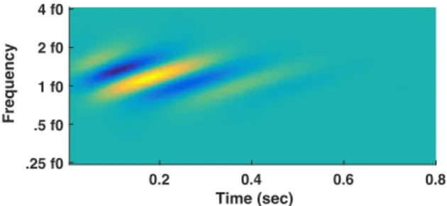
is the 2D inverse Fourier transform. The 4-dimensional output of the cortical stage is generated by convolving the auditory spectrogram with a bank of STRFs. Note, however, that fil-tering can be implemented more efficiently in the scale-rate domain. We denote this representation by Z(S, R, !, ⌧), where (S, R) gives the filter centers along the scale and rate axes. Figure 1 shows an upward moving STRF with a scale of 1 cycle per octave, and a rate of 4 Hz.
0.2 0.4 0.6 0.8 Time (sec) .25 f0 .5 f0 1 f0 2 f0 4 f0 Frequency 0.2 0.4 0.6 0.8 Time (sec) .25 f0 .5 f0 1 f0 2 f0 4 f0 Frequency
Fig. 1. An upward moving STRF, h*(!, ⌧ ; S = 1, R = 4).
The frequency is displayed on a logarithmic scale based on a reference frequency f0.
2.3. Multi-resolution Common Fate Transform
We address the invertibility issue, caused by the cochlear analysis block of the auditory model, through replacing the auditory spectrogram by a complex time-frequency represen-tation with log-frequency resolution. We use an efficient and perfectly reconstructable implementation of CQT, proposed by Sch¨orkhuber et al. [19]. The new 4-dimensional repre-sentation, denoted by ˆZ(S, R, !, ⌧ ), is computed by applying the cortical filter-bank of the auditory model to the complex CQT of the audi to signal. Note that the time-frequency representation can be reconstructed from ˆZ(S, R, !, ⌧ ) by inverse filtering as ˜ X(!, ⌧ ) =IFT2D ( P*+ S,Rz(s, r; S, R)Hˆ ⇤(s, r; S, R) P*+ S,R|H(s, r; S, R)|2 ) , (8)
where ⇤ denotes complex conjugate, ˆz(s, r; S, R) is the 2D Fourier transform of ˆZ(!, ⌧ ; S, R)for a particular (S, R), and P*+
S,Rmeans summation over the whole range of (S, R)
val-ues and all up-/down-ward filters. The next modification we make to improve the source separation performance is mod-ulating the filter bank with the phase of the input mixture. We know that components of |X(!, ⌧)| in the scale-rate do-main are shifted according to \X(!, ⌧). Assuming linear phase relationship between harmonic components of a sound, and hence linear shift in the transform domain, we expect to achieve better separation by using modulated filters, i.e. fil-ters with impulse responses equal to h(!, ⌧; S, R)ej\X(!,⌧).
3. EXPERIMENTS
In this section we compare the separability provided by the CFT and MCFT for mixtures of instrumental sounds playing in unison, but with different modulation patterns. For a quick comparison, an overview of the computation steps in the CFT and MCFT approaches is presented in Table 1.
3.1. Dataset
The main point of our experiments is to demonstrate the effi-cacy of the overall 4-dimensional representation in capturing amplitude/frequency modulation. We do not focus on the dif-ference in the frequency resolution of STFT and CQT over different pitches or octaves. Thus, we restrict our dataset to a single pitch, but include a variety of instrumental sounds. This approach is modeled on the experiments in the publica-tion where our baseline representapublica-tion (the CFT) was intro-duced [15]. There, all experiments were conducted on unison mixtures of note C4. In our work, all samples except one are selected from the Philharmonia Orchestra dataset2.
This dataset had the most samples of note D4 (293.66 Hz), which is close enough to C4 to let us use the same transform parameters as in [15]. Samples were played by 7 different instruments (9 samples in total): contrabassoon (minor trill), bassoon (major trill), clarinet (major and minor trill), saxo-phone (major and minor trill), trombone (tremolo), violin (vi-brato), and a piano sample recorded on a Steinway grand. All samples are 2 seconds long and are sampled at 22050 Hz. Mixtures of two sources were generated from all combina-tions of the 9 recordings (36 mixtures in total).
3.2. CFT and MCFT
To be consistent with experiments used for the baseline CFT [15], the STFT window length and overlap were set to ' 23 ms (512 samples) and 50%. The default patch size (based on [15]) was set to L! ' 172.3 Hz (4 bins ), and L⌧ ' 0.74
sec (64 frames). There was 50% overlap between patches in both dimensions. We also studied the effect of patch size on
Method Input Computation Steps Output CFT x(t) STFT ! 2D-windows centered at (⌦, T ) ! FT2D Y (s, r, ⌦, T )
MCFT x(t) CQT ! FT2D ! 2D-filters centered at (S, R) ! IFT2D Z(S, R, !, ⌧ )ˆ
Table 1. An overview of the computation steps in CFT and MCFT.
separation, using a grid of values including all combinations of L! 2 {2, 4, 8} and L⌧ 2 {32, 64, 128}. We present the
results for the default, the best, and the worst patch sizes. We use the MATLAB toolbox in [19] to compute CQTs in our representation. The CQT minimum frequency, max-imum frequency, and frequency resolution are respectively ' 65.4 Hz (note C2) and ' 2.09 kHz (note C7), and 24 bins per octave. The spectral filter bank, F (s; S), include a low pass filter at S = 2 3 (cyc/oct), 6 band-pass filters
at S = 2 2, 2 1, ..., 23 (cyc/oct), and a high-pass filter at
S = 23.5 (cyc/oct). The temporal filter bank, G(r; R),
in-clude a low-pass filters at R = 2 3 Hz, 16 band-pass filters
at R = 2 2.5, 2 2, 2 1.5, ..., 25 Hz, and a high-pass filter at
R = 26.25 Hz. Each 2D filter response, H(s, r; S, R),
ob-tained as the product of F and G is split into two analytic filters (see Section 2.2). The time constant of the temporal filter, , is set to 1 for the best performance. We have also provided a MATLAB implementation of the method3.
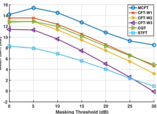
0 5 10 15 20 25 30 Masking Threshold (dB) -2 0 2 4 6 8 10 12 14 16 Mean SDR (dB) MCFT CFT-W1 CFT-W2 CFT-W3 CQT STFT
Fig. 2. Mean SDR for 2D and 4D representations versus masking threshold. 3 out of 9 patch sizes used in CFT compu-tation are shown: W1(2 ⇥ 128) (best), W2(4 ⇥ 64) (default),
and W3(8 ⇥ 32) (worst).
3.3. Evaluation via Ideal Binary Masking
To evaluate representations based on the amount of separa-bility they provide for audio mixtures, we construct an ideal binary mask for each source in the mixture. The ideal binary mask assigns a 1 to any point in the representation of the mix-ture where the ratio of the energy from the target source to the energy from all other sources exceeds a masking thresh-old. Applying the mask and then returning the signal to the time domain creates a separation whose quality depends only
3https://github.com/interactiveaudiolab/MCFT
on the separability of the mixture when using the representa-tion in quesrepresenta-tion.
We compute the ideal binary mask for each source, in each representation, for a range of threshold values (e.g. 0 dB to 30 dB). We compare separation using our proposed represen-tation (MCFT) to three variants of the baseline representa-tion (CFT), each with a different 2D window size applied to the STFT. We also perform masking and separation using two time-frequency representations: CQT and STFT.
Separation performance is evaluated via the BSS-Eval [20] objective measures: SDR (lower bound on separation performance), SIR, and SAR. Mean SDR over the whole dataset is used as a measure of separability for each threshold value. Figure 2 shows mean SDR values at different masking thresholds. MCFT strictly dominates all other representations at all thresholds. MFCT also shows the slowest dropping rate as a function of threshold. The values of objective measures, averaged over all samples and all thresholds are presented in Table 2, for STFT, CQT, CFT-W1 (best patch size), and
MCFT. CFT-W1 shows an improvement of 4.8 dB in mean
SDR over STFT , but its overall performance is very close to CQT. MCFT improves the mean SDR by 2.5 dB over CQT and by 2.2 dB over CFT-W1.
Method SDR SIR SAR STFT 5.2± 4.9 20.8± 5.1 5.7± 5.2
CQT 9.7± 5.4 23.4± 5.4 10.2± 5.7 CFT-W1 10.0± 4.9 24.4± 4.7 10.4± 5.2
MCFT 12.2± 3.9 24.1± 5.1 13.2± 4.7
Table 2. BSS-Eval measures, mean ± standard deviation over all samples and all thresholds.
4. CONCLUSION
We presented MCFT, a representation that explicitly rep-resents spectro-temporal modulation patterns of audio sig-nals, facilitating separation of signals that overlap in time-frequency. This representation is invertible back to time domain and has multi-scale, multi-rate resolution. Separation results on a dataset of unison mixtures of musical instru-ment sounds show that it outperforms both common time-frequency representations (CQT, STFT) and a recently pro-posed representation of spectro-temporal modulation (CFT). MCFT is a promising representation to use in combination with state-of-the-art source separation methods that currently use time-frequency representations.
5. REFERENCES
[1] M. Cooke, J. R. Hershey, and S. J. Rennie, “Monaural speech separation and recognition challenge,” Computer Speech & Language, vol. 24, no. 1, pp. 1–15, 2010. [2] S. Haykin and Z. Chen, “The cocktail party problem,”
Neural computation, vol. 17, no. 9, pp. 1875–1902, 2005.
[3] T. Heittola, A. Klapuri, and T. Virtanen, “Musical instru-ment recognition in polyphonic audio using source-filter model for sound separation.,” in ISMIR, pp. 327–332, 2009.
[4] J. F. Woodruff, B. Pardo, and R. B. Dannenberg, “Remixing stereo music with score-informed source separation.,” in ISMIR, pp. 314–319, 2006.
[5] M. D. Plumbley, S. A. Abdallah, J. P. Bello, M. E. Davies, G. Monti, and M. B. Sandler, “Automatic music transcription and audio source separation,” Cybernetics &Systems, vol. 33, no. 6, pp. 603–627, 2002.
[6] S.-W. Jeon, Y.-C. Park, S.-P. Lee, and D.-H. Youn, “Robust representation of spatial sound in stereo-to-multichannel upmix,” in Audio Engineering Society Convention 128, Audio Engineering Society, 2010. [7] D. Fitzgerald, “Upmixing from mono-a source
separa-tion approach,” in 2011 17th Internasepara-tional Conference on Digital Signal Processing (DSP), pp. 1–7, IEEE, 2011.
[8] S. Rickard, “The duet blind source separation algo-rithm,” Blind Speech Separation, pp. 217–237, 2007. [9] S. Rickard and O. Yilmaz, “On the approximate
w-disjoint orthogonality of speech,” in Acoustics, Speech, and Signal Processing (ICASSP), 2002 IEEE Interna-tional Conference on, vol. 1, pp. I–529, IEEE, 2002. [10] A. Liutkus, D. Fitzgerald, Z. Rafii, B. Pardo, and
L. Daudet, “Kernel additive models for source separa-tion,” IEEE Transactions on Signal Processing, vol. 62, no. 16, pp. 4298–4310, 2014.
[11] D. Fitzgerald, A. Liukus, Z. Rafii, B. Pardo, and L. Daudet, “Harmonic/percussive separation using ker-nel additive modelling,” in Irish Signals & Systems Conference 2014 and 2014 China-Ireland International Conference on Information and Communications Tech-nologies (ISSC 2014/CIICT 2014). 25th IET, pp. 35–40, IET, 2013.
[12] P. Smaragdis, “Non-negative matrix factor deconvolu-tion; extraction of multiple sound sources from mono-phonic inputs,” in International Conference on Inde-pendent Component Analysis and Signal Separation, pp. 494–499, Springer, 2004.
[13] P. Smaragdis, B. Raj, and M. Shashanka, “A proba-bilistic latent variable model for acoustic modeling,” Advances in models for acoustic processing, NIPS, vol. 148, pp. 8–1, 2006.
[14] A. S. Bregman, Auditory scene analysis: The perceptual organization of sound. MIT press, 1994.
[15] F.-R. St¨oter, A. Liutkus, R. Badeau, B. Edler, and P. Ma-gron, “Common fate model for unison source separa-tion,” in 41st International Conference on Acoustics, Speech and Signal Processing (ICASSP), IEEE, 2016. [16] T. Chi, P. Ru, and S. A. Shamma, “Multiresolution
spec-trotemporal analysis of complex sounds,” The Journal of the Acoustical Society of America, vol. 118, no. 2, pp. 887–906, 2005.
[17] L. Krishnan, M. Elhilali, and S. Shamma, “Segregating complex sound sources through temporal coherence,” PLoS Comput Biol, vol. 10, no. 12, p. e1003985, 2014. [18] P. Ru, “Multiscale multirate spectro-temporal auditory
model,” University of Maryland College Park, USA, 2001.
[19] C. Sch¨orkhuber, A. Klapuri, N. Holighaus, and M. D¨orfler, “A matlab toolbox for efficient perfect reconstruction time-frequency transforms with log-frequency resolution,” in Audio Engineering Society Conference: 53rd International Conference: Semantic Audio, Audio Engineering Society, 2014.
[20] E. Vincent, R. Gribonval, and C. F´evotte, “Performance measurement in blind audio source separation,” IEEE transactions on audio, speech, and language process-ing, vol. 14, no. 4, pp. 1462–1469, 2006.