FOR PASSIVE STABILIZATION by
R.J. Thome, R.D. Pillsbury, Jr., W.G. Langton, and W.R. Mann
Massaahusetts Institute of Technology Plasma Fusion Center
FOREWORD
This work was supported by the U.S. Department of Energy, Office of Fusion Energy under contract number DEA-D0278ET51013. It originally had limited distribution as Appendix B to FED-INTOR/MAG/82-2, which was sub-mitted as part of the U.S. contribution to Session V of INTOR, Phase IIA, Vienna, July 1982.
1. Introduction and Summary 2. Two Discrete Loops
2.1 Vertical Displacements 2.2 Radial Displacements 2.3 Time Constants
3. Toroidal Shells With Circular Cross Section (t = o+) 3.1 Vertical Displacements
3.2 Radial Displacements
4. Toroidal Shells With Noncircular Cross Sections 4.1 Complete and Incomplete Shells (t = o+) 4.2 Time Constants
S. Examples for INTOR
5.1 Discrete Loops for Vertical Stabilization 5.2 Discrete Loops for Radial Stabilization
5.3 Discrete Loops vs Complete Shells of Circular Section 5.4 Non Circular Partial Shells and Time Constants
1.0 INTRODUCTION AND SUMMARY
The vertical stabilization of an elongated plasma imposes severe require-ments on the system since the stabilizing magnetic field increment must be initially imposed on the time scale of the plasma displacement. It is usually not feasible to accomplish this with an active coil system alone because of the
excessive peak power which would be required. Consequently, stabilization using passive electrical coils, shells or shell segments has been under evaluation.
The general approach would be to allow the rapid plasma displacement to generate eddy currents in passive elements and produce an associated, induced magnetic field which would provide stabilization until the induced field could be augmented by an active control coil system. The latter would respond on a
longer time scale to limit peak power requirements to reasonable levels. This imposes two basic requirements on the passive stabilization system: (1) its
location and geometry must provide an induced. field of sufficient magnitude and (2) the induced field must be applied for a sufficient time interval.
This report presents results of an investigation into the means for
estimating the level of the induced fields and their associated time constants. In all cases, the plasma was represented by a single, circular current filament which could be displaced instantaneously either vertically or radially. The latter was considered for the sake of completeness even though the need for radial stabilizing elements is not anticipated at this time.
Section 2.0 considers the passive stabilizing elements to be two coils or discrete loops which are coaxial with the plasma filament and symmetrically located with respect to the z = 0 plane, the initial plane of the plasma.
induced currents and fields which result at t
=-o+
are derived in normalized form and presented in the form of contour plots to allow their estimationfor any specified loop location. These may be utilized with imposed restric-tions on location for a specific system to determine the most effective loca-tions and the level of interaction. The latter may then be compared with a stabilization requirement in terms of an induced field produced per unit dis-placement to determine if the magnitude of the interaction is sufficient.
Section 3.0 considers the effect of a complete passive shell around the plasma by presenting results for toroidal shells of circular section.
Ver-tical and radial displacements were considered and induced current distributions are given for typical cases to illustrate the most effective portions of the shells. Induced fields are given in a normalized form which is directly comparable to those used in Section 2.0. Results indicate that complete shells
can be about a factor of two more effective than discrete loops depending on shell aspect ratio.
The shells of circular cross-section in Section 3.0 are analytically tractable for the t = o+ instant and useful for providing insight into the problem. However, shells for tokamaks such as INTOR, which utilize elongated plasmas, are unlikely to be circular. Hence, Section 4.0 presents the results for complete and partial shells of a more suitable geometry. Field results are again presented in a normalized form suitable for comparison with previous sections.
Section 5.0 contains examples using the results of the previous three sections to illustrate methodology and generate estimates based on INTOR (Phase
1) characteristics. Section 5.1 uses a simplified stability criterion to de-termine location for discrete passive, vertical stabilization, loops to provide
-3-an interaction of sufficient strength. Results show that locations along cer-tain sections of the first wall or blanket outer boundary are adequate, but that no location as far out as the shield outer boundary is sufficient. Time constants are also estimated and indicate that values of the order of several seconds or lower are achievable depending on toroidal continuity, material cross-section and electrical conductivity. Hence, considerable flexibility exists for adjusting this time constant to be compatible with field penetration and excita-tion times for active stabilizaexcita-tion coils.
Discrete loops are compared with toroidal shells of circular section in Section 5.3 which shows the shells to be substantially more effective. In addi-tion, it should be noted that the field produced by a distributed element such as a shell is likely to be much more uniform over a greater volume than that pro-duced by discrete loops. This may be an advantage when more realistic plasma
characteristics are considered.
Noncircular complete and partial shell segments are related to INTOR in Section 5.4 with shell locations within, but near the blanket outer boundary
and at the outer shield boundary. The former location is adequate and the latter is not, when effectiveness is compared with the same simple requirement utilized for loops in Section 5.1. Time constants are estimated and again show that considerable flexibility is possible depending on selection of shell
thickness and material.
The models utilized in this work were selected to allow mathematical trac-tability and to generate insight for this problem. Although they are simplified,
they indicate general trends and means for normalization to allow results to be applied or scaled to other cases. Future work requires improved plasma modeling to investigate dynamic effects.
0 N
4.. -0 'I-N N i f
I
L. 0 1.~ N a.-' NC>
'-4 0 I ,\\,
1-40if
~ I
1
ON 4.) (A 0 . 4J -o c~J 1.. I
-5-2.0 TWO DISCRETE LOOPS
This section will present estimates of the fields produced by induced currents in two co-axial, passive coils as a result of the instantaneous ver-tical or radial displacement of a plasma. The plasma is modeled as a single circular current filament. Curves are given which allow the estimation of the induced current magnitude as well as the radial field due to a vertical displace-ment of the plasma and the vertical field induced by a radial displacedisplace-ment.
Time constants for induced current (or field) decay are given for both cases and are not equivalent unless the two passive loops are closely coupled.
2.1 Vertical Displacements
The model used in this section is shown in Fig. 2.1. The plasma is re-presented by a single circular current filament of radius ro which is located in the z = o plane for t < o and which instantaneously moves a distance Az parallel to the z-axis at t = o. Two coaxial, conducting loops of radius a are located with planes at z = d. The left sketch in Fig. 2.1 shows the di-mensions of the model in real space whereas the right sketch illustrates the model in a space with dimensions normalized to the plasma radius.
For t < o the plasma is operating with a steady-state current I in the z = o plane and the current in the passive loops is zero. At t = o the plasma moves a distance, Az vertically and induces currents of magnitude I in the loops.
If it is assumed that Ip is constant, the induced current may be shown to be given by
I = I (Z\eTG (1)
where Ip = plasma current
t = time
T = t/T 0 (2)
T =
(L-M)/R
(3)
L = self inductance of one passive loop M = mutual inductance between passive
loops
R = resistance of one passive loop
The induced current is proportional to the displacement and to the plasma current, and decays with a time constant, T . It is also dependent
on G which is primarily a function of the dimensionless coordinates which locate the passive loops, that is,
49 [(1 + P)2 +2 3/2 -K/k2 + E)
(
G I= (1-k 2) k k.. 4 (n 8a - 7 2 ( - k 2/2)K - E ." )'
T jok.
-7 rW 0LJwhere
T =d/ro
P = a/roK, E = Complete elliptic integrals with modulus, k
K E0= Complete elliptic integrals with modulus, ko
r = Effective radius of cross-section of passive loop
k = p [p2 + n21-1/2
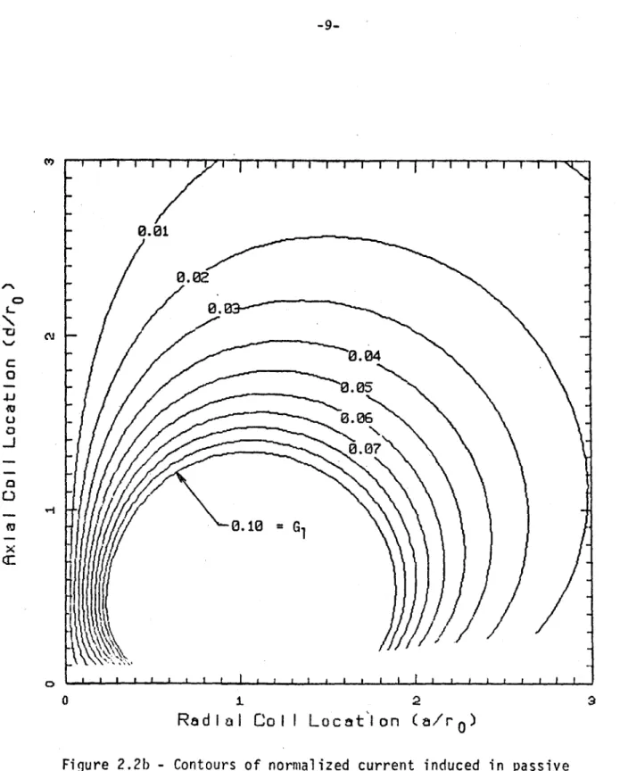
-7-The function Gl may be considered to be a normalized current at t = o+. Con-tours of constant Gi are shown in Figs. 2.2a and 2.2b in (a/ro, d/ro) space. Passive loops located at (a,d) may be located in this diagram once the plasma radius, ro is specified. The contour which passes through the point then gives the value of GI for use in (1) to determine the induced current in the passive loops. The diagram assumes that (a/rw) = 20, that is, the loop cross-sectional dimension is snall relative to the loop radius, a, and their ratio is the assumed constant regardless of location in the diagram.
The derivation of (1) assumes that the loops are continuous as shown in Fig. 2.1 and the left sketch in Fig. 2.3. However, if the current paths are formed from saddle coils so that the toroidal path is discontinuous as in the right sketch in Fig. 2.3 then (1) and Fig. 2.2 can still be used to estimate the induced current at t = o+ provided the "legs" of adjacent saddle coils are close together. The time constant for current decay of the saddle coils will be substantially shorter than To for the complete loops because of the
added resistance of the legs. An example of this type is considered in Section 5.1.
The radial field at the plasma as a result of the induced currents given by (1) may be shown to be
B = 10IP
Ai
e G (5)r
r
r
where: o= permeability of free space = 4Tr x 10-7 [H/m]
CO L
-o
em -0. =G1 x -0.2 - 0.3-0. 0RndIaI CoII LocatIon (a/r(
si ur 2.2a
Co
ntours of normalized current induced in passive
plasma displacemcent. (See Eqn. 1Y.' (No& a/ a =e20).o vria
-9- 0.01-0.02 0. CM 0. 10 =G 0 2 a
Rad Ia I Co I I Locat'l on (a/ro)
Figure 2.2b - Contours of normalized current induced in passive stabilizing coils located at ( alro, d/ro) as a result of a vertical plasma displacement. (See Eqn. 1) . Note: (a/r w) = 20.
Od
00
u-C(120
"0,14
1.
0 0 0 " 0 00 0>
Cu bo jILc
tn
0
2-
020
LJ- 0 C)u cs0 0
-- -11-0
-o
G2
0
~ 0.2 x 00 0.0
1 2RadIal Col
I
Location
(a/ro)
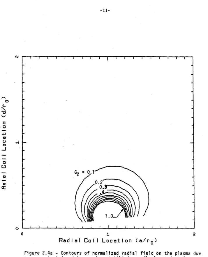
Figure 2.4a
-Contours of normalized radial field on the plasma due
to currents induced in passive stabilizing coils located at
(a/ro,
d/r
)
as a result of vertical plasma displacement. (See Eqn. 5).
The radial field is thus proportional to plasma current and displacement and also decays with the time constant, TO. It is dependent on G2, a function de-pendent primarily on the dimensionless location of the loops which is given by
16 pn2 [(l+p) 2 + 12] -K/k2 + E [l 26
28a 2 (6)
_r _L(
), -1 kC) K -E
rw 4 k0 2 0-0
The radial field provides a vertical restoring force on the plasma and the function G2 may be considered to be a normalized radial field at t = o+
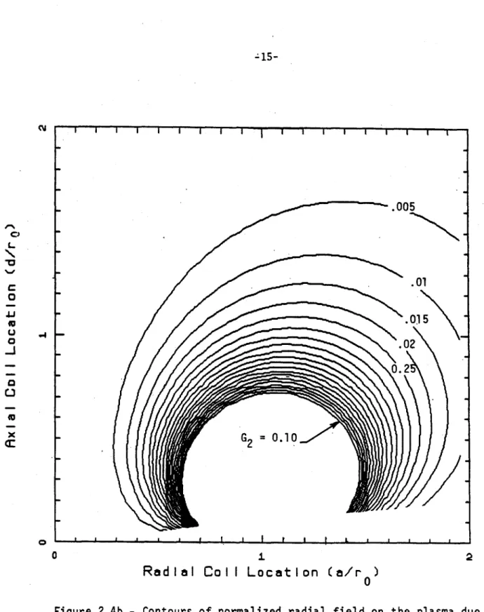
Contours of constant G2 are plotted in Figs. 2.4a and 2.4b. Loops with coor-dinate locations (a,d) may be located in this diagram once the plasma radius is specified. In the diagram the plasma is located at (0,1) and the contour value G2 determines the strength of the field produced by the induced currents in the loops when used with (5). A constant a/rw = 20 is again used.
The contour diagram may be used with an overlay which "deletes" areas in which passive loops cannot be located because of system constraints. The maximum contour values in "allowable" areas may then be used to determine the best location for passive loops. An estimation can then be made directly of the radial field which can be produced for a given displacement to deter-mine if the interaction is of sufficient magnitude. This process is illus-trated with an example in Section 5.1.
-13-2.2 Radial Displacements
The model used in this section is shown in Fig. 2.5. The plasma is represented by a single circular current filament of radius r 0 which is lo-cated in the z = o plane and which instantaneously moves a radial increment, 6, at t = o. Two co-axial, conducting loops of radius "a" are again located with planes at z = d. The left sketch in Fig. 2.5 shows the dimensions of the model in real space whereas the right sketch illustrates the model in a space with dimensions normalized to the plasma radius.
For t < o the plasma is operating with a steady-state current Ip at a radius r and the current in the passive loops is zero. At t = o, the plasma moves radially to (r + 6), its current changes to I', and it induces currents
0 p
of magnitude I in the loops. Note that I circulates with the same sense in both loops in this case, whereas the currents were of opposite sense for vertical plasma displacements in the previous section. The induced current may be shown to be given by
I =T I' G (7)
p r 03
0
where: T= t/To
T = (L + M)/R (8)
Note the difference in time constant for this case relative to the previous case (ie-compare (8) and (3)) because of the symmetric versus antisymmetric
induced currents. The function, G., is primarily.dependent on the dimension-less coordinates of the loops and is given by:
SP/2 K/k2 + E k2p [ 2P(l+P) -COG 4 (9)
G -(1-k) (l+p)2 + T12 I(l+P)2 + T 2
3 In (a) Tw - 7
4
+2k
K E0
2~
0EJ1
where4 G
i
p(/2 (1-k 2/2) K E] (10)1/2 for constant flux expansion
C = 0 . for constant energy expansion (11)
-l/2 for constant current expansion
The choice of the constant C0 is dependent on whether the plasma is as-sumed to expand at constant flux, energy or current. For example, the flux produced by the plasma current filament may be assumed to be the same before
and after the expansion, in which case C = 1/2.
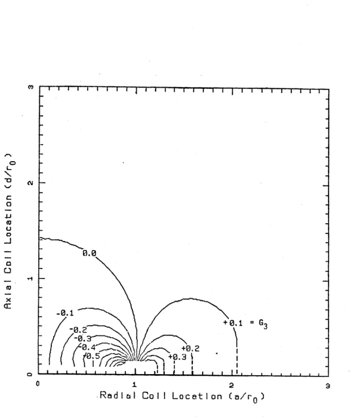
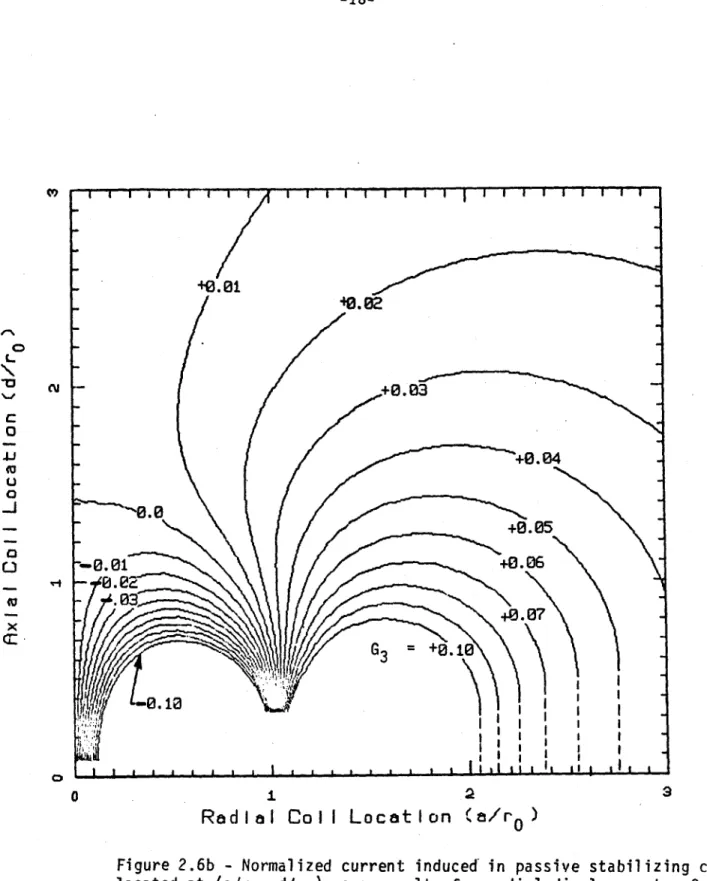
The function G3 may be considered to be a normalized current at t = o+ Contours of constant G3 are shown in Figs. 2.6a and 2.6b in (a/ro ,d/r ) space for the case where C = 1/2 (constant flux). Passive loops with coordinates (a,d) may be located in this diagram once the plasma radius is specified. The contour which passes through the point then gives the value of G for use in
(7) to determine the induced current in the passive loops. The diagram is
based on (a/r
)
= 20, that is, the loop cross-sectional dimension is smallre-lative to the loop radius, a, and their ratio is the assured constant
regard-less of location in the diagram except as
n
= o where curves are extrapolated because of errors introduced by expressions for inductance in this range.The presence of a G3 = o contour should be noted in Figs. 2.6a and b. This
implies that the direction of the induced current is dependent on loop location. This leads to the possibility of developing a destabilizing force instead of a stabilizing force and will become apparent in the figures which follow.
,15-.005
C3 L .01002
4J-0.2
- G2 0.10a2
Rad
Ial
Co
I
Location (a/r
)
0
Figure 2.4b
-Contours of normalized radial field on the plasma due
to currents induced in passive stabilizing coils located at (a/ro,
d/r
0) as a result of vertical plasma displacement. (See Eqn. 5).
0
I00
N
0.0
(k
CN
s-v
~~1
~II.
- u.-1----I - I --K)
H-
-~ 0 NA
~
-f
1\J
IIUP
0n
,K)
0K)4
tv 0 4J a; * + o 0 S. 4J 0E - S-o 0 to -r-Eu . -W > ca) r-0 > e- e CA 0-4J0 In Eu I A I-17-0 L
-o
(a
U0.0
-+0.1 = G3 -0.1 4 +0.2 0.5 +0.3 0 i 23
,Radl l Co
I I
LocatIon (a/r
0
)
Figure 2.6a - Normalized current induced in passive stabilizing
coils located at (a/r 0, d/ro) as a result of a radial displacement.
Contours correspond to C = 1/2 (i.e. - constant flux produced by
++..0 CD 0..03 0+. 2 +0.04 (U 0.0 -+0.05
r3
1
o
-.
oi
+0.06- .2
+0.07 X G3 =.+0.1 -0.10RadIal
Coll Location
(
)/r0
Figure
2.6b
-
Normalized current induced in passive stabilizing coils
located at (a/ro, d/ro) as a result of a radial displacement.
Contours
correspond to Co
=
1/2
(i.e. - constant flux produced by the
plasin).
-19--01 C --0.1 - G5>Oo ,6.6..A 02
Rad
I
al
Co
I
I Locat
I
on
(a/r
0
Figure 2.7a
-Normalized Z-directed field due to current induced
in stabilizing coils located at (a/ro, d/r
)
as a result of a radial
plasma displacement. Contours correspond ?o C
0 =1/2 (i.e.
-constant
The z-directed field at the plasma as a result of the induced currents given by (7) may be shown to be:
Bz r/Gr5 (12) where G = G /2 + k [-K/k2 + E ()/(1-k 2 x k _ _2(1+p)_ [(l+p)2 + n2] [(l+p)2 + (2]2 13)
The induced z-field is thus proportional to plasma current and displacement and decays with the time constant T'. It is dependent on G5, a function
de-00
pendent primarily on the dimensionless coordinates of the loops and on C0 (through G), the assumption governing the manner in which the plasma expands.
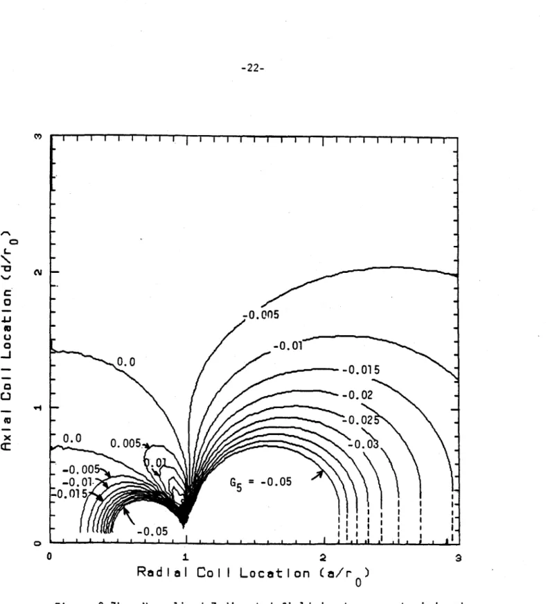
G5 may be considered to be the normalized z-directed field at the plasma at t = o+. Contours of constant G5 are plotted in Figs. 2.7a and 2.7b for a constant flux expansion. Loops with coordinates (a,d) may be located in this diagram once the plasma radius, r0, is specified. In the diagram, the plasma
is located at (o,1) and the contour value G5 determines the strength of the
field produced by the induced currents in the loops when used with (12). A
constant a/rw = 20 is again used in (13) to construct the contours. except as T = o is approached where curves are again extrapolated.
A positive plasma current (i.e.-into the diagram) in Figs. 2.7a or 2.7b requires
a negative Bz for stabilization. This corresponds to a negative G5 . The diagrams
show that loops may be located so as to be stabilizing (G5 < 0) or destabilizing (G5 > 0), hence, positioning passive coils in the latter region should be avoided.
-21-The position of the destabilizing zone is strongly dependent on the
as-sumption made concerning plasma action when displaced. The figures discussed
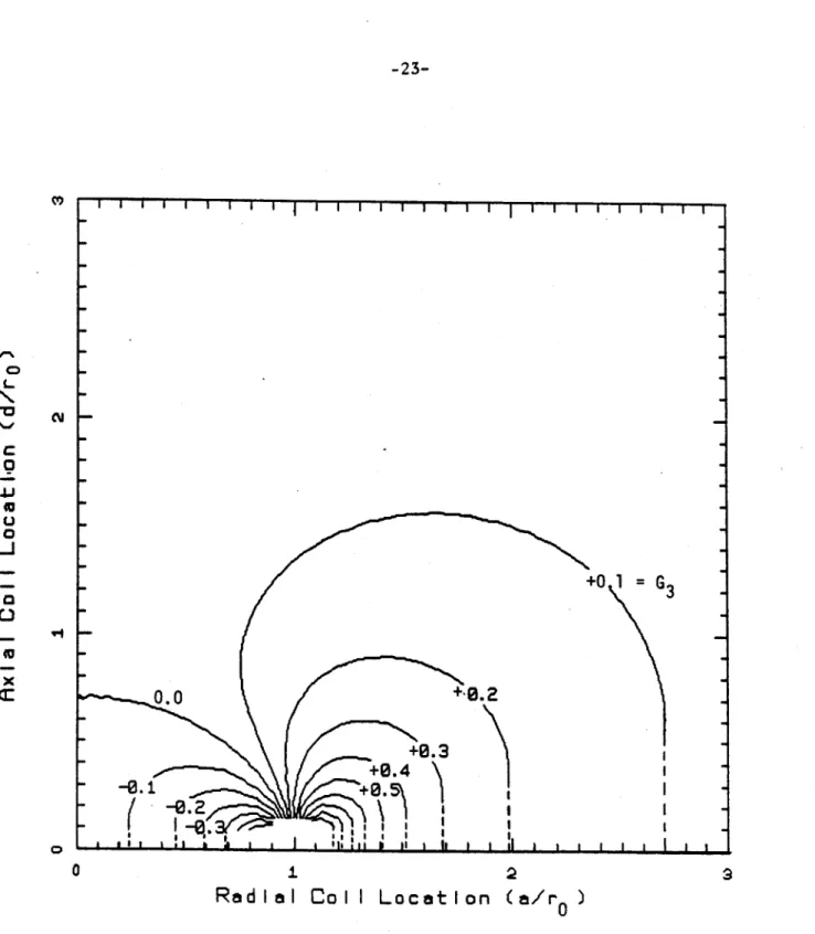
thus far assume that the flux produced by the plasma current is the same be-fore and after displacement (C = 1/2). If, on the other hand, it is assumed that the plasma current remains constant then Figs. 2.8 and 2.9 can be generated for G3, normalized current, and G, normalized z-field. The latter exhibits no destabilizing zone for passive coil location and illustrates the qualitative difference in results due to different assumptions regarding plasma character when the expansion take place.
The contour diagrams (eg-Figs. 2.7a and b) for G5 may be used with an
overlay which "deletes" areas in which passive loops cannot be located because
of system constraints. The maximum stable contour values in "allowable" areas may then be used to determine the best location for passive loops and an esti-mation can be made of the vertical field which can be produced for a given displacement to determine if the interaction is of sufficient magnitude. This process is illustrated with an example in Section 5.2.
The derivation of (7) and (12) assumes that there are two loops as shown in Fig. 2.3 and that they are toroidally continuous. If a segmented design
is desired for radial stabilization, the type of saddle coil arrangement shown
in Fig. 2.3 for vertical stabilization cannot be used, because currents in-duced by radial plasma displacement are of like sense above and below the z = o plane, hence, no currents would flow. It is, therefore, necessary to base the coil segments for radial stabilization on a four loop system as shown
in Fig. 2.10. The left sketch shows a four loop system which is continuous and the right sketch shows a segmented coil set. The currents induced in the
I I I II i1 I i 1 1 1 1 1 1 1 I
-0.
0.0
0.005.
-0.00
-0.01--0.015
-0.05-0.005
-0.01
-0.015
-0.02
-002
I-4' I2
a
Radial
Coil
Location
(a/r)
0
Figure 2.7b
-
Normalized Z-directed field due to currents induced
in stabilizing coils located at (a/ro, d/ro) as a result of a radial
plasma displacement. Contours correspond to Co
=1/2 (i.e.
-
constant
flux produced by the plasma). (See Eqn. 12).
(Note: a/rw
=
20).
0-L 0 -I-a: N' '-4 0 0"
-G5 =
0.05
-23-I -23-I I I I I I I I I I I I I1 I I I I I I I I I I I- m +~
6.+
0.0 + 0.2+0.3
1 +0-..
I, aa
a i I
Im a a
i
Radial
CollI
Location
0 3 = G II I a (a/r)0
a
Figure 2.8
-
Normalized current induced in passive stabilizing coils
located at (a/r
0, d/ro) as a result of a radial plasma displacement.
Contours correspond to Co
=-1/2 (i.e.
-constant plasma current).
(See Eqn. 12). (Note: a/rw
=20).
0D L-'U 0 0 x
a:
CMI TI9 0 0i
a i
I
I I I II I II I, I I liii II I~j I III 11111
.-
0.05
- .5-0.1 .. 0.0-0.05
-0.
-0.1
0.A1 0.5 I 2Rad
lal
Co
II
Locatlon (a/r0)
Figure 2.9
-
Normalized Z-directed field due
stabilizing coils located at (a/ro, d/ro) as
plasma displacement. Contours correspond to
plasma current). (See Eqn. 12). (Note: a/rw
to currents induced in
a result of a radial
Co
=
-1/2 (i.e.
-
constant
=
20).
L C 4JI 'U U 0x
'-f 0 0 9 I 1 4 . . a - I a A I . I = G 5- -25-4-b -r4 4J 0 00 00 .. JU 0
00
0~ 04 0 + -r4U 0 V..40 00 4J0 -4 Cd' r*r4segmented coil set at t = o+ would be the same as in the four loop continuous set provided the radial connections of adjacent segments were close together, however, the currents would decay with faster time constants because of the added resistance of the radial connectors between loops.
The contour plots given in this section were based on a two loop system. They may be used as a first approximation to estimate the characteristics for a four loop set as shown in Fig. 2.10 by superposition of contour values for G and G However, this approach for 4 loops will neglect the inductive
3 S
coupling between the inner and outer loops and may be expected to yield opt-imistic z-fields at t = o+. Decay time constants will also be altered.
2.3 Time Constants
The previous two sections derived induced currents and fields for two loop systems and showed that the time constant for decay of induced fields was not the same for the case of vertical vs radial plasma displacements. This is attributed to the different symmetry of the induced currents relative to the z = o plane which is manifested as mutually aiding or mutually opposing induced flux. The time constants are given by:
DISPLACEMENT DECAY TIME CONSTANT
Vertical To = (L-M)/R
Radial T' = (L+M)/R
0
These time constants may be shown to be of the form
-27-T =
pa
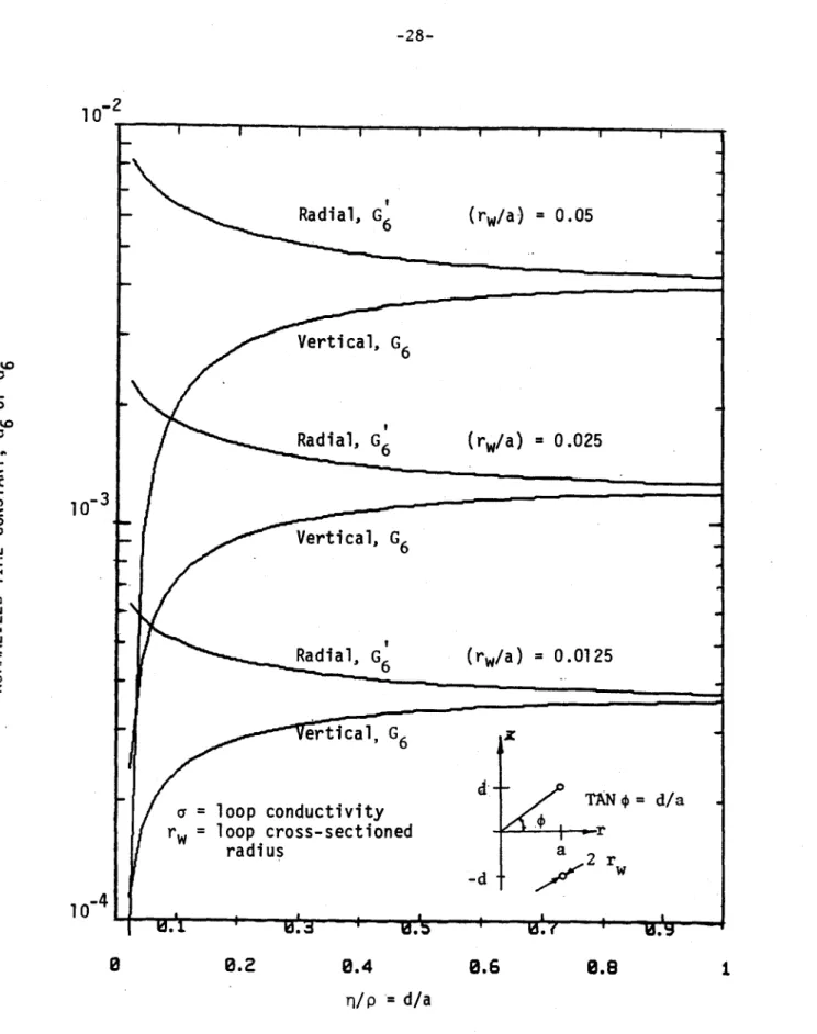
a2 G6 (d/a, r /a) (15) where a = conductivity of passive coil materialThe functions G6 and G6 may be considered to be dimensionless time constants.
They are plotted in Fig. 2.11 as a function of the ratio of loop coordinates. Curves in Fig. 2.11 are based on constant values of rw/a'= 0.05, 0.025 and 0.0125. There is also an implicit assumption that the induced current is uni-formly distributed over the loop current carrying cross-section of radius, rw. For large values of d/a, the loops are far apart, hence, there mutual induc-tance is small and the time constants for both cases approach the same value. As d/a - o, the loops approach the z = o plane and M + L, thus the time
con-stants diverge. For d/a = o, the two loops merge into one and no current is in-duced by a small vertical plasma displacement whereas a current may still be induced by a radial plasma displacement.
If saddle coils are used for vertical stability as shown in Fig. 2.3, in-stead of two continuous loops, then (14) may still be used to estimate the time constant for current decay. However, To is shortened by the added resis-tance of the saddle legs, hence, To from (14) should be multiplied by
C 1 + s w (16)
2a As
where:
k = number of saddle coils
2.s= length of one saddle coil "vertical" leg
As = effective cross-sectional area of one saddle coil leg for current flow
2
10-Vertical, G 6 10-CD I-CDRadial,G
(r /a)
=0.0125 6 6 01 U - Vertical, G6 Ui < RadialA, G .02 d/aa rw loop cross-sectioned radius a 2 r -d -44 10 0 0.2 0.4 0.6 0.8ri/p
= d/aFigure 2.11
-
Time constants for toroidally continuous passive
-29-Equation (16) assumes that the saddle coil legs have the same conductivity as the loop material.
This section has derived time constants for induced current and field de-cay from passive loops following a single, step function in displacement of the plasma loop. Ultimately, the plasma must be dynamically stabilized. When the dynamic interaction is considered the time constants for growth or suppres-sion of an instability may be expected to be related to, but somewhat different from the time constants in this section. However, this approach allows the relative effectiveness of different passive loops to be evaluated on an approx-imate basis and allows an insight to be gained into the important parameters.
3.0 TOROIDAL SHELLS WITH CIRCULAR CROSS SECTION (t = o+)
Section 2.0 considered the passive stabilization effects of two discrete current loops symmetrically placed relative to the z= o plane and developed contour plots which can be used to estimate the magnitude of the induced current and fields. However, passive stabilization coils which are more distributed in nature, for example, plates, shell segments or complete shells, may be more likely
to be used if more uniform induced stabilization fields are desired.
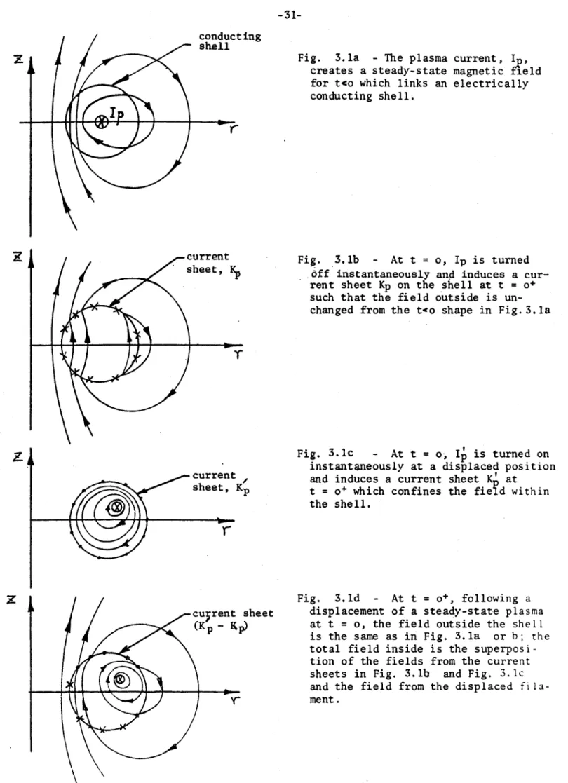
Some insight into the characteristics of a complete shell problem can be gained by considering the t - o+ induced current distribution and stabilizing field magnitude which results from plasma displacement within a toroidal shell of circular section. The results in this section assume that the effects of a small plasma displacement on the shell can be modeled by superposition of the simultaneous and instantaneous turn off of the steady-state plasma at its undis-placed position and turn on at its disundis-placed position. The method of finding
the induced current in the shell at t = o+ due to turn off at t = o, may be found in Thome and Tarrh ; the currents induced by a turn on may be found in a similar fashion since they are the negative of those in a turn off problem. The super-position process is illustrated and described in Fig. 3.1. The induced current
and fields at the plasma filament location following a displacement may be expressed as two infinite series involving toroidal coordinates and Legendre
associated functions. Partial sums of these series were evaluated over a range of shell parameters for small vertical and radial plasma displacements. General
results are given in this section and examples using these results are given in
Section 5.3.
R.J. Thome and J.M. Tarrh, MHD and Fusion Magnets: Field and Force Design Concepts, John Wiley, New York. 1982, p. 256.
-31-conducting
shell
Fig. 3.la - The plasma current, I creates a steady-state magnetic field for t<o which links an electrically conducting shell.
Fig. 3.1b - At t = o, Ip is turned 6ff instantaneously and induces a cur-rent sheet Kp on the shell at t = o+
such that the field outside is un-changed from the two shape in Fig. 3.la
'r
Fig. 3.lc - At t = o, I is turned on instantaneously at a displaced position and induces a current sheet K' at
t = o+ which confines the fie d within the shell.
cuyrent sheet (Kp -
~p)
'_0
Fig. 3.ld - At t = o+, following a displacement of a steady-state plasma
at t = o, the field outside the shell is the same as in Fig. 3.la or b; the total field inside is the
superposi-tion of the fields from the current sheets in Fig. 3.lb and Fig. 3.1c and the field from the displaced fila-ment. vi,.
x
current sheet, KPr'
4r
current sheet, YI3.1 Vertical Displacements
The range of shell parameters and initial, undisplaced plasma positions which were evaluated using the series referred to in the previous section is illustrated in Fig. 3.-2. The shell geometry is determined by the ratio of its major to its minor axes, R/r m. The dimensionless initial plasma location is determined by the ratio of the plasma filament radius to the major axis of the shell, r 0/R. The scale of the system may then be found by specifying any
one of the dimensions, R, rm or r .
A small vertical displacement of the plasma from the z = o plane induces currents in the shell which tend to have opposite signs above and below the z = o plane and thus produce a radial field tending to return the plasma to its initial position. The current sheet amplitude at t = o+ is of the form
K =2 G7 (17)
where:
K = local current sheet amplitude (e g.- in [A/m]) AZ = small vertical displacement
G 7 = G 7 (R/rm, r /R, C)
The function G7 may be considered to be a normalized local current sheet
amp-litude and is plotted in Figs. 3.3. and 3.4 for shells with R/r = 2 and R/rm = 4, respectively. Three curves are shown on each plot and correspond to initial plasma locations of r /R = 0.9, 1.0 and 1.1. Relative scale for the different cases may be visualized with the aid of Fig. 3.2. In each case, negative current is induced in the top of the torus and positive current in
-33-r.=.
0.9
R
1.0
4I.'
2.
Toroidal Conducting Shells with Circular Section; the plasma is initially located in the z=o plane at radius ro.
r
=4
~3
7
0.9
1.0
1.1
ofI
II
y~n Figure 3.20.
1.0 1.1
1
I
R/y
4-y
i5r- --- -- - - - f- - - I - - - -:-- - - - - - ,-- - -T,--ro/R-O. 9 4j. 3 So/R-10 2 r -I~
~~
-IC--4
-2L
-G-
- 4-o --4 - - -$0 5~~ 5 -L-20-100
0
100
2
* (deg)
Fig. 3.3
-Induced Current Sheet for Vertical Plasma
Displacement for a Shell with R/r
=2.
-35-20 r - - - --r -- - --- - - -- -T - -
-~/R=8.9
1. 51 - - - -- --- -- -R/-1.0 I I I1 -5... Z--- --T) r-
1
(**) G-20 L
-
-4U-
-
- -
-
--~I
5 I I -200 -100 0 100 200 * (deg)Fig. 34
-Induced Current Sheet for Vertical Plasma
the bottom of the torus, thus producing a positive radial field which will tend to push the plasma filament (positive current and positive AZ) back toward the z = o plane. Note that the area of current concentration is relatively localized for each case, thus implying that a partial shell at that location would be
almost as effective as the complete shell. However, the area of concentration is also relatively sensitive to initial plasma filament location which suggests that a distributed plasma current model would produce induced currents which were much less concentrated.
The induced radial field at the plasma location at t = o+ has the form:
Br =( )( AZ G8 (18)
where:
G8 = G8 (R/rm,ro/R) (19)
The function G8 may be considered to be the normalized induced radial field
due to the small vertical displacement and is directly comparable to G2 for loops (e.g.-see eqn.5) It is plotted in Fig. 3.5 as a function of R/rm for selected values of r /R. When R/rm and r /R are specified, G8 may be found and used with (18) to find Br following specifications of Ip, r0, and AZ.
3.2 Radial Displacements
A small radial displacement of the plasma filament in the z = o plane induces currents in the shell which tend to have opposite signs on the outside and inside extremes of the shell cross-section and thus produce a vertical
field which tends to return the plasma to its initial position. The current sheet amplitude at t = o+ is of the form:
-3,7-V
00
-03
0 I 2 3 - 4 55HELL
ASFECT RATIO
R/r
Figure 3.5 Normalized Radial Field vs. Shell Aspect Ratio for Three Cases of Plasma Filament Initial Position; see Eq. (18).
/I \,Ar\
K = G 9 (20)
where: Ar = small radial displacement
0
9
= G9 (R/rM, r /R,$)The function Gg may be considered to be a normalized local current sheet
amplitude. It was generated assuming that the plasma produces the same amount
of flux before and after expansion. G% is plotted in Figs. 3.6 and 3.7 for shells with R/rm = 2 and R/rM = 4, respectively. In each case, negative cur-rent is induced on the far outside of the toroidal shell and positive curcur-rent on the far inside, thus producing a negative z- directed field which tends to push the plasma filament (positive current and positive Ar ) back toward its initial position. Note that the current concentration is more localized to-ward the outside for r /R = 1.1 and more toward the inside for r /R = 0.9.
The induced z- directed field at the plasma location at t = o* has
the form
B = -r 0 G10 (21)
where:
G 60= G10 (R/r m, r /R) (22)
The function 610may be considered to be the normalized induced t- directed
field due to the small radial displacement, Ar . It is plotted in Fig. 3.8 as a function of R/r for selected values of r /R. When R/r and r /R are
m o m 0
specified, G1 0may be found from Fig. 3.8 and used with Eqn.(21) to-find Bz
-39-Gg
4L-0 - - --
- --ro /R=-. .9 -2r-r- - -- -- - - - -r 0 R1.0 -6 ~ r ~IT -200 -100 0 100 200 $(deg)
Fig.3.6 - Induced Current Sheet for Radial Plasma
L- - - -- - - r - - -
-I
II
II
I
I
10 CD I I- I 1O/R . -: I I -5- --- I- o/R-1.0 I- --- 4 -- -- 4 -- --4.) S -15 L --- L -- - -- - - l _ e-I agI -25l ~ ~ i ~ ~ 1.I /R-1.I-200
-100
0
100
200
$(deg)
Fig.
3.7- Induced Current Sheet for Radial Plasma
Displacement for a Shell with R/rm = 4
-41-RADIAL DIbPLACEtE 4T
R
1.0
0.9
3
2
Figure 3.8SHELL AoPECT RATIO, R/'r
Normalized Vertical Field vs. Shell Aspect Ratio for Three Cases of Plasma Filament Initial Position; see Eq. (21).
a
LIT
G
a
0
-a.U
4
I4.0 TOROIDAL SHELLS WITH NONCIRCULAR CROSS SECTIONS
The previous section presented results for toroidal shells with circular cross sections to gain insight into: 1) the regions where induced currents flow on complete shells when a plasma is displaced and 2) the difference in the
magnitude of the induced fields relative to those achieveable with the discrete loops of Section 2.0. The main advantage to the approach in Section 3.0 is that the model may be treated with standard analytical techniques. The dis-advantages are that results are limited to the t = o+ instant, the shell is complete and the shell is of circular cross section.
In this section a finite element model* is used with toroidal shells that have complete and incomplete noncircular sections to more realistically re-present likely configurations for passive stabilization coils or shell seg-ments. Toroidal continuity is assumed throughout this section and only ver-tical plasma displacements are considered. Figure 4.1 shows the location of the shells considered and of the plasma which is modeled with a rectangular cross section of uniform current density. We will again assume that a small, rapid vertical displacement of the plasma may be adequately modeled by a rapid turn off of the plasma at its steady state position and simultaneous turn on at its displaced position. This may be shown to be exact in the limit of a very small displacement.
4.1 Complete and Incomplete Shells (t = o+)
Sections 2.0 and 3.0 showed that, for small displacements, the induced fields and currents were proportional to the plasma current, the displacement and a dimensionless function describing the geometry of the passive conduct-ing material and plasma location. In Section 3.0 the dimensionless function
*R.D. Pillsbury, "A Two-Dimensional Planar or Axisymmetric Finite Element Program for the Solution of Transient or Steady, Linear or Non-Linear Magnetic Field Pro-blems," COMPUMAG, Chicago, Sept. 1981.
-43-for a circular section shell was dependent on ro/R (plasma location) and on R/r (shell geometry). One complete shell of the type shown in Figure 4.1
m
would require four dimensionless parameters to describe its geometry and one to describe initial plasma location if the plasma were modeled as a single
filimentary loop. A more complex plasma model would require additional para-meters to describe its geometry. Furthermore, at t = o+, the induced currents are generated on the shell surface so its thickness does not enter into the function. However, the shell thickness is important at later times because it affects the decay time constant.
In view of the above, we would expect to be able to normalize the induced radial field at t = o+ for a shell (or shell segment) of the type shown in Fig. 4.1 to (p I p/r ) and to (AZ/r ) as was the case in Sections 2.0 and 3.0 The normalized values based on calculations from the finite element model will constitute a function, G . Radial fields at t = o+ for other cases with different plasma currents, displacements or shell size may then be found by
scaling from
Br G (23)
t= 0+(
provided the shell is geometrically similar to the shell used in obtaining G . This is somewhat more restrictive than for the previous sections where the passive elements could be described by a single dimensionless ratio and the functions could be expressed analytically. In this case, the function
cannot be found analytically, but can be found using the finite element method then scaled to other geometrically similar cases.
The function Gl is plotted in Fig. 4.2 for the inner shell and for the outer shell as shown in Fig. 4.1. The intersection of each curve with the ver-tical axis is the result for a complete shell. As a curve progresses from
side. The angle subtended by the shell is the horizontal axis and is defined in the insert sketch. Points on the sketch are labeled to correspond to points on the curve. The curves are relatively flat for large subtended angles thus implying
that the inboard segments are relatively ineffective in producing radial field. The region 0%, 30* is also relatively ineffective. The relatively large difference between inner and outer shells is consistent with the trend shown in Fig. 3.5 for
complete shells with circular sections with different aspect ratios, R/rm
In general, one would expect to generate comparable radial field magni-tudes at a point with a complete shell or an effectively placed shell segment. However, more complete shells would be expected to produce a more uniform radial field distribution over a larger region within the shell.
4.2 Time Constants
Selected cases based on Fig. 4.1 were computed to determine field de-cay in time. Results are plotted in Fig. 4.3. Four lines are shown, each corre-sponding to a copper shell or shell segment as indicated in the inset sketches.
The top curve represents a complete inner shell and the second curve is for an inner shell segment which occupies a relatively effective region. The latter case exhibits a relatively rapid initial-decay of the higher harmonic content of its induced current pattern, then decays at about the same time con-stant as the top curve. A curve fit to the top two curves to estimate a single
time constant yields 3.13 sec for the top curve and 2.94 sec for the second. The cases represented by the lower curves correspond to the outer shell and yield a lower level radial field because they are not as well coupled to the plasma. Part of the outer shell segment chosen for the lower-curve is in a relatively ineffective region. A curve fit to the two lower curves to estimate
-45-inner shell
outer shell
plasma
3 4 S 8 7R (
m)
B 910
Fig. 4.1
-
Two Shell Finite Element Model for Plasma Displacement
Study; The plasma has a rectangular cross-section and
uniform current density and produces the field lines
shown in the ste-ady state before plasma displacement.
'-I E N -4 co 0 i 22 3 J 1.0 3 45 2" .91 .8-2 3
inner shell
7only
.6 U 4j) 3 .outer she11
only 0 0 .2 -3 18U .50 120 90 60 30Angle Subtended by Shell,
s
Figure 4.2 -Normalized Radial Magnetic
F
'ield Due to a Plasma Vertical
Displacement for Complete and Incomplete Shells based '6n
-47-0 C A A 0 * ts 4-J -A U' (ft L-S C C 4 i f m
S/7
S. 0 a A (D A 0 C r +a 4 W--b ,0-4 C .a.0 %n 4') o N Ne N LL. * .,-*4-b U - W +am -o 4.h w W 41 0-. - a4-h E qu o b-CL E -4Q a. o 0 e--C * en .C toLt 4a. a. E 0U -0 SL'. I-/ I-,'I
W 4. W a. axi
'P L
Ltped
PaztL~w.AON-a single time const-ant yields 1.39 sec for the third curve and 0.93 seconds for the fourth curve. These time constants may be scaled for other geometri-cally similar shells or segments by assuming that the time constant is pro-portional to shell thickness and inversely propro-portional to shell resistivity. The results assume toroidal continuity and all portions of a shell must be
scaled by the same constant. If saddle coils are used, the impact on the time constants may be estimated using a method similar to that in Eq. (16).
Note that complex geometries can not strictly speaking,be described by a single time constant since they are, in effect, a collection of multiple coupled circuits. However, the current components with the faster time
con-stants decay earlier; hence, a curve fit toward the end of a transient allows a single time constant to be estimated.
-49-5.0 EXAMPLES RELATED TO INTOR
5.1 Discrete Loops for Vertical Stabilization
This section will illustrate the use of the general material developed in Section 2.1 to estimate the characteristics of two passive loops for stabilization in INTOR. Results show that the most effective location is on the first wall and that locations on the shield outer boundary are too
far from the plasma to be effective. Maximum possible time constants for induced field decay are also estimated for continuous loops and for saddle coils (see Fig. 2.3).
Contours of dimensionless radial field induced by a vertical plasma displacement were developed in Section 2.1 and presented in Figs. 2.4a and b. Figure 5.1 is the same as Fig. 2.4a, but shows three boundaries corresponding to the location of the first wall, outer blanket boundary (assuming a 0.5 m thick blanket), and outer shield boundary (assuming a 1.0 m shield with 0.1 m gap between blanket and shield) for INTOR. Points A, B and C represent maximum values of the function G2 on the inner boundary, blanket outer boundary, and shield outer boundary, respectively. They are, therefore, the most effective points for location of passive vertical stabilization coils on each of these boundaries. The contour values at these points are given in the third line in Table 5.1. If we now assume a plasma major radius of r = 5.3 m and current
I = 6.4 MA, the baseline INTOR parameters, then Eq. (5) may be used with the p
G2 values from Table 5.1 to estimate the maximum possible induced radial field per unit vertical displacement which can be generated by loops located on one
of the three boundaries. Results are given in line 4 in Table 5.1. These are values at t = o and decay with time constant T 0 (See (5)).
TABLE 5.1 - CHARACTERISTICS OF VERTICAL
STABILIZATION COILS AT Pts A, B AND C IN FIG. 5.1
1. 2. 3. 4. 5. 6. 7. 8. 9. 10. 11. 12. Point Location G2 (Fig. 5.1) B r/(AZ) [T/M] Loop Radius, a [m] Loop z Coord, d [m] d/a G6 (Fig. 2.11)
t0 max for loops, [sec]
S, [m]
*
T max for saddles, [sec]
os
based on 12 saddle coils
A B C
First Wall Blanket Outer Shield Outer
Boundary Boundary 0.72 0.38 0.13 0.20 0.11 0.036 6.15 6.52 7.26 1.59 2.01 2.76 0.26 0.31 0.38 3.1 x 10⁻³ 3.3 x 10⁻³ 3.5 x 10⁻³ 8.55 10.2 13.4 3.5 4.45 6.25 4.09 4.43 5.08 0.30 0.334 0.413
-51-The value of B r/(AZ) which is required may be estimated* by assuming that this induced field per unit displacement is equal in magnitude to the applied, steady-state value of (aB /az). r Using the definition of the field index the requirement may be expressed as
/(A Za (24)
r eqd r where:
B Za applied steady-state vertical field n = field index
If we assume n = -0.95 and BZa = -0.5 T then [B /(z)reqd = 0.089 T/m. Com-parison of this requirement with line 4 in Table 5.1 indicates that it can be exceeded at points A or B, but cannot be achieved at point C. The criterion
implies, therefore, that passive vertical stabilization by two loops cannot be achieved with locations on the shield outer boundary but could be achieved using locations at points A or B with considerable "excess" field production or by locating loops on any contour with G2 > 0.31 which corresponds to
[Br/(AZ)]reqd = 0.089 T/m.
Maximum possible time constants for loops located at points A, B and C can be estimated using Fig. 2.11 as follows. Loop radius, a, z-coordinate, d, and the ratio d/a for points A, B and C are given in lines 5, 6 and 7 in Table 5.1. Values of the normalized time constant, G6, from Fig. 2.11 are given in
line 8 assuming (rw/a) = 0.05. If we now assume that the coils are copper which in turn, specifies the conductivity, a, then Eq. (4) may be used to determine the time constant T for points A, B and C. This is given in line 9 and has been labeled a maximum since materials with lower conductivity could be used and because line 9 corresponds to a large conductor cross-sectional area, A, for each
loop (see line 12).
The latter arises implicitly since A = Trw where rw is the effective conductor radius and since the curves selected from Fig. 2.11 are for rw/a = 0.05. Lower
time constants than those in line 9 may therefore be achieved by using a poorer conductor and/or decreasing A by decreasing (rw/a) and using a different curve from Fig. 2.11.
The time constant, T0 in line 9 assumes that the loops are toroidally con-tinuous as illustrated in the left sketch in Fig. 2.3. Maximum possible time constants for saddle type coils (right sketch in Fig. 2.3) may now be estimated using Eq. (5). These will be estimated by assuming that the saddle legs are also copper and that the leg conductor cross section is the same as that for the loop (i.e.-line 12 in Table 5.1). Twelve saddle coils will be assumed and the length of a single leg of the saddle, Z., is assumed to be twice the dis-tance from the loop to the z = 0 plane along the boundaries shown in Fig. 5.1. The length, Zs, for each point is given in line 10 and the estimated maximum time constant for saddle coils, T os in line 11 in Table 5.1. Results indicate that the maximum achievable time constants are relatively long and could be adjusted downward by using a conductor with higher resistivity and/or smaller conductor cross-sectional areas.
This section has estimated the characteristics of two loops for passive vertical stabilization for INTOR. Results indicate that considerable flexi-bility in loop location exists to develop a sufficient interaction based on a simplified stability criterion. Points along large sections of the first wall boundary and outer blanket boundary have sufficient capability, but points along the shield boundary do not. Estimates of maximum possible time constants
indicate that either continuous loops or saddle type coils are suitable and that there is considerable flexibility available for adjustment of the time
-53-5.2 Discrete Loops for Radial Stabilization
Elongated plasmas such as those envisioned for INTOR are generally be-lieved to be radially stable under usual operating conditions and, therefore, do not require discrete loops for radial stabilization as discussed in Section 2.2. However, this section will utilize INTOR dimensions to illustrate the use of the contours presented in Fig. 2.7.
Figure 5.2 is identical to Fig. 2.7a except that the INTOR dimensions have been used to outline the first wall, blanket outer boundary and shield outer boundary. G5 contours represent normalized z-directed field at the
plasma position due to currents induced in discrete loops located on a parti-cular contour. Maximum field occurs with loops located on the maximum allow-able contour. For the three boundaries, the maximum contour values occur at points A, B and C on the midplane of the machine although there is essentially no change in effectiveness if the loops are located slightly off the midplane.
Contour values for points A, B and C are given in Table 5.2, line 3. These values may now be used with Eq. (12) to determine the induced field per unit
radial displacement (line 4) which could then be compared with a suitable sta-bility requirement to estimate whether the interaction with discrete loops was
sufficiently strong. Time constants could be derived using (15) in a manner similar to that used in the previous section.
L U w shield outer 0 boundary
-j
0 blanket outer -~boundary
01 G .3 INTOR inner boundaryRadial ColI Location (a/r0
Figure 5.1 INTOR boundaries superimposed on Normalized Radial Field Contours (see figures 2.4a and 2.4b); A, B and C show most effective locations on boundaries for passive loops for vertical stabilization.
-55-i
AB
C
2 9RadIal
Coll
Location (a/rO)
Figure 5.2 - INTOR boundaries superimposed on Normalized
.z-directed
Field Contours (see Figures 2.7a and 2.7b.L-A, B,.,and
C show moqst effectiye 1qcat.Qon.
gri.- undaries for
passive loops for rgdial stabilization if required;
Contours assume plasma expansion at constant flux
(Co
=
1/2) see Equation (12).
to,
-I AI II
shield outer boundary
~
blanket outer boundary
INTOR inner boundary
-G5 > 0 0.0 - 0.050. -0.05 = G5
--
0.1
- .
-- 0.15
0.1
-
-0.5
0 41 L 0 ... 0 0TABLE 5.2 - CHARACTERISTICS OF RADIAL
STABILIZATION COILS AT Pts A, B AND C IN Fig. 5.2
Point Location G5 (Fig. 5.2) Bz/6 [T/M] Loop radius, a [m] Loop z - coord, d [m] A First Wall 0.87 0.25 6.63 0 B C
Blanket Outer Shield Outer
Boundary Boundary 0.49 0.20 0.14 0.05 7.12 8.23 0 0 1. 2. 3. 4. 5. 6.
-57-5.3 Discrete Loops vs Complete Shells of Circular Section
The toroidal shells of circular cross-section in Section 3.0 are of in-terest since the solutions illustrate the manner in which the induced fields will scale and Figs. 2.16 and 2.19 show the strength of the dependence of the normalized field functions on the aspect ratio of the shells. They are also useful for estimating the difference in the strength of the induced field from loops relative to that which could be obtained from a complete shell at the instant immediately following the plasma displacement. The time constants for decay of the induced fields would be expected to be different for the two cases.
Figure 5.3a is the same as Fig. 2.4a which showed contours of dimension-less radial field for discrete loops. Three complete toroidal shells with dif-ferent aspect ratios are superimposed on the contours. The dimensionless radial field which can be produced by each of these shells is G8 which may be found in Fig. 2.16. Values for ro/R = 1.0 were used and are given in Table 5.3, line 2a. The corresponding function for discrete loops is G2 and the maximum values
for G2 outside any one of the shells may be found in Fig. 5.3a as points A, B
and C. These values are given in Table 5.3 in line 2b. Results indicate
that a shell with aspect ratio R/rm = 3, for exaihple, can produce 1.5 times
the radial field which can be produced by a pair of discrete loops at the most effective location outside the same shell envelope.
A similar approach was used in Fig. 5.3b which is the same as Fig. 2.7a for radial stabilization by discrete loops. Table 5.3 gives the dimensionless
z-field function, G10 for shells and the directly comparable maximum G5 for
loops on the shell boundaries. Results again show that the shells are substan-tially more effective.
TABLE 5.3 - EFFECTIVENESS OF DISCRETE LOOPS VS TOROIDAL SHELLS OF CIRCULAR SECTION
1. Shell Geometry, R/rm 2 2.5 3.0
2. Vertical Stabilization
a. G8 for shell 0.51 0.81 1.25
b. G2 max for loops 0.28 0.5 0.88
c. Shell/loops 1.82 1.62 1.42
3. Radial Stabilization
a. G10 for shell -0.55 -0.85 -1.28
b. G5 max for loops -0.24 -0.37 -0.52