Climate change, mortality and adaptation : evidence from annual fluctuations in weather in the U.S.

Digitized

by

the

Internet

Archive

in

2011

with

funding

from

Boston

Library

Consortium

IVIember

Libraries

^DEWEY

Massachusetts

Institute

of

Technology

Department

of

Economics

Working Paper

Series

Climate

Change,

Mortality

and

Adaptation:

Evidence

from

Annual

Fluctuations

in

Weather

in

the

U.S.

Olivier

Deschenes

Michael

Greenstone

Working

Paper

07-1

9

June

21,

2007

Room

E52-251

50

Memorial

Drive

Cambridge,

MA

02142

This

paper can be

downloaded

without

charge

from

the

Social

Science Research

Network

Paper

Collection

at

Climate

Change,

Mortality,

and

Adaptation:

Evidence

from

Annual

Fluctuations in

Weather

in the

US*

Olivier

Deschenes

UniversityofCalifornia,Santa Barbara

Michael

Greenstone

MIT

and

NBER

June

2007

*

We

thank the late

David

Bradford for initiating a conversation that motivated this project.

Our

admiration for David's brilliance as an economist

was

only

exceeded

by

our admiration for

him

as a

human

being.

We

are grateful for especially valuable criticisms

from

Maximillian

Auffhammer, David

Card,

Hank

Farber,

Ted

Gayer, Jon Guryan,

Solomon

Hsiang, Charles Kolstad,

David

Lee, Erin

Mansur,

Enrico Moretti, Jesse Rothstein,

Bernard

Salanie,

Matthew

White and

Catherine

Wolfram.

We

are also grateful for

comments

from

seminar participants at several universities

and

conferences. Elizabeth

Greenwood

provided truly outstanding research assistance.

We

also thank

Ben Hansen

for

exemplary

researchassistance.

We

are verygratefulto the British

Atmospheric

Data

Centre forprovidingaccessto

the

Hadley

Centre data.

Greenstone

acknowledges

the University ofCalifornia

Energy

Institute

and

the Center for

Labor Economics

at

Berkeley

for hospitality

and

supportwhile

working on

thispaper.

Climate

Change,

Mortality,

and

Adaptation:

Evidence

from

Annual

Fluctuationsin

Weather

in the

US

ABSTRACT

This paper produces the first large-scale estimates ofthe

US

health related welfare costs

due

to climate change.

Using

the

presumably

random

year-to-year variation in temperature

and

two

state

of

the art climatemodels,the analysissuggeststhat

under

a 'business asusual' scenarioclimate

change

will leadto

an increase in the overall

US

annual

mortahty

rate ranging fi-om

0.5%

to

1.7% by

the

end of

the

ZT*

century.

These

overall estimates are statistically indistinguishable

from

zero, although there is evidence

ofstatistically significant increases in mortality rates for

some

subpopulations, particularly infants.

As

the canonical

Becker-Grossman

health productionfunction

model

highlights, the fullwelfare impactwill be reflected in health

outcomes and

increased

consumption

of

goods

that preserve individuals' health.

Individuals' likely first

compensatory

response is increaseduse ofair conditioning; the analysis indicates

thatclimate

change

would

increase

US

annualresidentialenergy

consumption by

a statisticallysignificant

15%

to 30%) ($15to

$35

billion in

2006

dollars) atthe

end

ofthe century. It

seems

reasonableto

assume

that the mortality impacts

would

be larger without the increased energy consumption. Further, the estimated mortality

and

energy impacts likely overstate the long-run impacts

on

these outcomes, since individuals can

engage

in a wider set of adaptations in the longer run to mitigate costs. Overall, the analysis suggests that the health related welfare costs of higher temperatures

due

to climate

change

are

likely to

be

quite

modest

inthe

US.

Olivier

Deschenes

Department

of

Economics

2127

North

Hall Universityof

Cahfomia

Santa Barbara,

CA

93106-9210

email: olivier@econ.ucsb.edu

Michael

Greenstone

MIT,

Department

of

Economics

50

Memorial

Drive,

E52-39IB

Cambridge,

MA

02142

and

NBER

Introduction

The

climate is a

key

ingredient in the earth's

complex

system that sustains

human

life

and

well

being. There is a

growing

consensusthatemissions of greenhouse gases due to

human

activity will alter

the earth's climate,

most

notably

by

causing temperatures, precipitation levels,

and weather

variability to

increase.

According

tothe

UN's

IntergovernmentalPanel

on

Climate

Change

(IPCC)

Fourth

Assessment

Report, climate

change

is likely to affect

human

health direcdy through

changes

in temperature

and

precipitation

and

indirectly through changes in theranges ofdisease vectors (e.g., mosquitoes)

and

other channels

(IPCC

Working Group

II, 2007).

The

design of optimal climate

change

mitigation policies

requires credible estimates of the health and other benefits of reductions in

greenhouse

gases; current

evidence

on

the

magnitudes

of the direct

and

indirect impacts, however, is considered insufficient for

reliableconclusions

(WHO

2003).'

Conceptual

and

statistical

problems

have

undermined

previous efforts todevelop estimatesofthe

health related welfare costs ofclimate change.

The

conceptual

problem

is that the canonical

economic

models

ofhealth production predict that individuals will respond to climate

changes

thatthreaten their

health

by

purchasing

goods

that mitigate the health

damages

(Grossman

2000). In the extreme, it is

possible that individuals

would

fully "self-protect" such that climate

change

would

not affect

measured

health outcomes. In this case, an analysis that solely focuses

on

health

outcomes would

incorrectly concludethatclimate

change had

zeroimpact

on

welfare.

On

the statistical side, there are at least three challenges. First, there is a complicated,

dynamic

relationship

between

temperature

and

mortality,

which

can cause the short-run relationship

between

temperature

and mortahty

to differ substantially

from

the long-run

(Huynen

et al. 2001;

Deschenes

and

Moretti 2007)." Second, individuals' locational choices

—

which

determine

exposure

to a climate

—

are related to health

and socioeconomic

status, so this

form

ofselection

makes

it difficult to uncover the

'

See Tol (2002a and 2002b) for overall estimates ofthe costs ofclimate change,which areobtained by

summing

costs over multiple areas including

human

health, agriculture, forestry, species/ecosystems, and sea level rise.

Deschenes and Greenstone (2007) provides evidence on the impacts on the

US

agricultures sector. Also, see

Schlenker,

Hanemann,

andFisher (2006).

^_{For example,Deschenes andMoretti (2007) documenttheimportance of forward displacement or "harvesting"on}

causal relationship

between

temperature and mortality. Third, the relationship

between

temperature

and

healthishighlynonlinear

and

likely tovary acrossagegroups

and

other

demographic

characteristics.

This paper develops

measures

ofthe welfare loss associated withthe directrisks to health posed

by

climate change in the

US

that confront these conceptual

and

statistical challenges. Specifically, the paper reports

on

statistical

models

for

demographic

group

by

county mortality rates

and

for state-level

residential energy

consumption

(perhapsthe primary

form

ofprotection againsthigh temperaturesvia air conditioning)that

model

temperature semi-parametrically.

The

mortality

models

include county andstate

by

year fixed effects, while the energy ones include state

and

Census-division

by

year fixed effects.

Consequently, the temperature variables are identified

from

the unpredictable

and presumably random

year-to-year variation in temperature, so concerns about omitted variables bias are unlikely to be important.

We

combine

the estimated impacts of temperature

on

mortality and energy

consumption

with predicted changes inclimate

from

'business as usual' scenariostodevelop estimates ofthe health related

welfare costs ofclimate

change

in the

US.

The

preferred mortality estimates suggest an increase in the

overall annual mortality rate ranging

from

0.5%

to

1.7% by

the end of the century. These overall estimates are statistically indistinguishable

from

zero, although there is evidence of statistically

significant increases in mortality rates for

some

subpopulations, particularly infants.

The

energy results

suggestthat

by

the end ofthe century climate changewill causetotal

US

residential energy

consumption

to increase

by

15%i - 30%). This estimated increase is statistically significant, and,

when

valued at the averageenergyprices

from

1991-2000,itimpliesthattherewillbe anadditional

$15

-

$35

billion(2006$)

peryearof

US

residentialenergy consumption.

Overall, the analysis suggests that the health related welfare costs of higher temperaturesdue to

climate

change

will be quite

modest

in the

US.

The

small

magnitude

ofthe mortality effects is evident

when

they are

compared

to the approximately

1%

per year decline in the overall mortality rate thathas

prevailed over the last 35 years. Further, it

seems

likely that the mortality impacts

would

be larger

withoutthecompensatory increase inenergy consumption. Finally, itisevidentthatanexclusive analysis ofmortality

would

substantiallyunderstate the health relatedwelfarecostsof climate change.

Thereare a

few

important caveatstothese calculations and,

more

generally, tothe analysis.

The

estimated impacts likelyoverstate the mortality

and

adaptationcosts, becausethe analysis relies

on

inter-annual variation in weather,

and

less expensive adaptations (e.g.,migration) will be available in response

to

permanent

climate change.

On

theotherhand, the estimated welfare losses fail to include the impacts

on

other health-relateddeterminantsof welfare(e.g., morbidities) that

may

be

affected

by

climatechange,

so in this sense they are an underestimate. Additionally, the effort toproject

outcomes

atthe

end

ofthe century requires a

number

of strong assumptions, including that the climate

change

predictions are

correct, relative prices (e.g., forenergy

and

medical services) willremain constant, the

same

energy

and

medical technologies will prevail,

and

the

demographics

ofthe

US

population (e.g., age structure)

and

their geographical distribution willremain

unchanged.

These

arestrong assumptions, buttheirbenefit is

thattheyallowforatransparent analysisbased

on

data rather than

on

unverifiableassumptions.

The

analysis is

conducted

with the

most

detailed

and comprehensive

data available

on

mortality,

energy consumption, weather,

and

climate

change

predictions for fine

US

geographic units.

The

mortality data

come

from

the

1968-2002

Compressed

Mortality Files,the energy data are

from

the

Energy

Infomiation Administration,

and

the weather data are

from

the thousands of weather stations located

throughoutthe

US.

We

focus

on

two

sets of

end

of century (i.e.,

2070-2099)

chmate change

predictions

that represent "business-as-usual" or

no

carbon tax cases.

The

first is fi^om the

Hadley

Centre's 3rd

Ocean-Atmosphere General

Circulation

Model

using the Intergovernmental Panel

on

Climate

Change's

(IPCC)

AlFl

emissions scenario

and

the

second

is

from

the NationalCenterfor

Atmospheric

Research's

Community

Climate

System

Model

(CCSM)

3 using

IPCC's

A2

emissionsscenario.

Finally, it is notable that the paper's

approach

mitigates or solves the conceptual

and

statistical

problems

that have

plagued

previous research. First, the availabihty of data

on

energy

consumption

means

that

we

can

measure

the impact on mortality

and

self-protection expenditures. Second,

we

demonstratethat the estimation of annual mortality equations, ratherthan daily ones, mitigatesconcerns

aboutfailing to capture the full mortality impacts of temperature shocks. Third, the county fixed effects

adjust for any differences in

unobserved

health across locations dueto sorting. Fourth,

we

model

daily temperature semi-parametrically

by

using 20 separate variables, so

we

do

not rely

on

functional

form

assumptionsto inferthe impacts ofthehottest andcoldest days onmortality. Fifth,

we

estimate separate

models

for 16

demographic

groups,

which

allows for substantial heterogeneity in the impacts of

temperature.

The

paper proceeds as follows. Section I briefly reviews the patho-physiological and statistical

evidence on the relationship

between

weather

and

mortality. Section II provides the conceptual

framework

for our approach. Section III describes the data sources and reports

summary

statistics.

Section

IV

presents the econometric approach, and Section

V

describes the results. Section

VI

assesses the

magnitude

of our estimates of the effect of climate change and discusses a

number

of important caveats tothe analysis. SectionVII concludesthepaper.

I.

Background

on

the Relationship

between

Weather and

Mortality

Individuals' heat regulation systems enable

them

to cope with high

and

low

temperatures. Specifically, high and

low

temperatures generally triggeran increase in the heartrate in orderto increase blood flow

from

the

body

totheskin, leading to the

common

thermoregulatory responses of sweating in

hot temperatures and shivering in cold temperatures.

These

responses allow individuals to pursue

physical

and

mental activities without endangering their health within certain ranges of temperature.

Temperatures

outsideofthese rangespose dangersto

human

health and can resultinprematuremortality.

This sectionprovidesa briefreviewofthe

mechanisms and

thechallengesforestimation.

Hot

Days.

An

extensive literature

documents

a relationship

between

extreme temperatures

(usually during heat

waves)

and mortality (e.g., Klineberg 2002;

Huynen

2001;

Rooney

et al. 1998).

These

excess deaths are generally concentrated

among

causes related to cardiovascular, respiratory,

and

cerebrovascular diseases.

The

need for

body

temperature regulation

imposes

additional stress on the cardiovascular

and

respiratory systems. In terms of specific indicators of

body

operations, elevated

temperatures are associated with increases in blood viscosity and blood cholesterol levels. It is not surprising that previous research has

shown

that access to air conditioning greatly reduces mortality

on

hotdays

(Semenza

etal. 1996).

immediately caused

by

a period of very high temperatures is at least partially

compensated

for

by

a

reduction inthe

number

ofdeathsin the periodinmiediately subsequent to thehot day ordays

(Basu

and

Samet

2002;

Deschenes

and

Moretti 2007). This pattern is calledforward displacementor "harvestmg,"

and

itappears to occur becauseheat affects individuals that

were

already very sick

and

would

have

died

in the near term. Since underlying health varies with age, these near-term displacements are

more

prevalent

among

theelderly.

Cold Days.

Cold

days are also a risk factor formortality.

Exposure

to very cold temperatures

causes cardiovascular stress dueto changes in

blood

pressure, vasoconstriction,

and

an increase inblood

viscosity (which can lead to clots), as well as levels of red blood cell counts,

plasma

cholesterol,

and

plasma

fibrinogen

(Huynen

et al. 2001). Further, susceptibility to

pulmonary

infections

may

increase

because breathing coldaircan leadtobronchoconstriction.

Deschenes and

Moretti (2007) provide the

most comprehensive

evidence

on

the impacts of cold

days onmortality.

They

find"evidence ofa large

and

statistically significant effect

on

mortahty within a

month

ofthe cold

wave.

This effect appears to be largerthan the

immediate

effect, possibly because it

takes time for health conditions associated with

extreme

cold to manifest themselves

and

to spread" (Deschenes

and

Moretti 2005). Thus, inthecaseof cold weather, it

may

be thatthereare delayed impacts

and

that the full effect of a cold day takes a

few

weeks

to manifest itself Further, they find that the

impact is

most pronounced

among

the

young

and

elderly

and

concentrated

among

cardiovascular

and

respiratory diseases.

Implications.

The

challenge forthis study

and any

study focused

on

substantive changes inlife expectancy is to

develop

estimates ofthe impact of temperature

on

mortality that are based

on

the full

long-runimpact

on

life expectancy. Inthe caseofhot days, theprevious literature suggeststhat thistask

requires purging the temperature effects ofthe influence ofharvesting or forward displacement. In the caseof cold days, the mortahty impact

may

accumulate

over time. Inboth cases, the

key

point isthatthe

fullimpactofagiven day's temperature

may

take

numerous

daysto manifestfully.

Our

review of the literature suggests that the full mortality impacts of cold

and

hot days are

section outlines a

method

that allows the mortality impacts of temperature to manifest themselves over longperiodsoftime. Further, the

immediate

and

longer runeffectsofhot

and

colddays arelikely tovary

across the populations, with larger impacts

among

relatively unhealthy subpopulations.

One

important determinant of healthiness is age, with the old

and

young

being especially sensitive to environmental

insults. Consequently,

we

conduct separate analyses for 16

demographic

groups defined by the interactionof

gender

and

8 agecategories.

II.

Conceptual

Framework

In principle, it is possible to capture the full welfare effects

of

climate change through

observations

on

the land market. Since land is a fixed factor, it will capture all the differences in rents

associatedwith differences inclimate

(Rosen

1974).''

The

advantage ofthis

approach

is thatin principle the full impact of climate

change

can be

summarized

in a single market. Despite the theoretical and

practical appeal ofthis approach, it is unlikely to provide reliable estimates ofthe welfare impacts of

climatechange.

We

base thisconclusion

on

a seriesofrecentpapersthatsuggest thattheresults fi^orathe

estimation of cross-sectional hedonic equations for land prices are quite sensitive to seemingly

minor

decisions about the appropriate control variables, sample, and weighting

and

generally appear prone to

misspecification (Black 1999;

Chay

and

Greenstone

2005;

Deschenes

and

Greenstone

2007; Greenstone and Gallagher 2007).

An

alternative approachis todevelopestimatesofthe impact ofclimatechangeina

seriesofsectors,

which

could then be

summed.

This paper's goal is to develop a partial estimate ofthe health related welfare impact ofclimate

change. This section begins by reviewing a

Becker-Grossman

style 1-period

model

ofhealthproduction

(Grossman

2000). It then uses the results to derive apractical expression forthe health relatedwelfare

impacts of climate

change

(Harrington

and

Portney 1987). This expression guides the subsequent

empirical analysis.

The

section then discusses the implications of our estimation strategy that relies on

inter-annual fluctuations inweatherforthe

development

ofthesewelfare estimates.

A

Practical Expression for Willingness to

Pay

/Accept

(WTP/WTA)

for

an

Increase in

^

Temperature.

We

assume

a representative individual

consumes

a jointly aggregated

consumption

good,

Xc- Theirother

consumption

good

istheirmortalityrisk,

which

leadstoautilityfunction

of

(l)U

=

U[xc,s],

where

s isthesurvivalrate.

The

productionfunction forsurvivalisexpressedas:

(2) s

=

s(xh, T),

so survival is a function ofXh,

which

is a private

good

that increases the probability of survival,

and

ambient

temperature, T.

Energy consumption

is an

example

of Xh, since energy is used to run air

conditioners,

which

affect survival

on

hot days.

We

define xh such that 9s/9xh

>

0. For expositional purposes,

we

assume

that climate

change

leads to an increase in temperatures inthe

summer

only

when

highertemperatures areharmfulforhealth sodsldl

<

0.

The

individual facesabudget constraintofthe form:

(3)I

-

Xc

-

pxH

=

0,

where

I is

exogenous

earnings or

income and

prices of xc

and

Xh are 1

and

p,respectively.

The

individual's

problem

isto

maximize

(1) through her choices of Xc

and

xh, subjectto (2)

and

(3). In equilibrium, the ratioofthemarginalutilities of

consumption

ofthe

two must be

equaltotheratio

of the prices: [(5U/9s)-(9s/5xh)]/[5U/i9xc]

=

p. Solution ofthe

maximization

problem

reveals that the

input

demand

equationsforxc

and

xh arefunctions ofprices,

income, and

temperature. Further,itreveals

the indirect utihty fimction, V,

which

isthe

maximum

utihtyobtainablegivenp, I,

and

T.

We

utilize V(p, I, T) to derive an expression forthe welfare impact of climate change, holding

constant utility (and prices). Specifically,

we

consider changes in

T

as are predicted to occur under

climate change. In this case, itis evidentthatthe

consumer

must

be compensated

for changes in

T

with

changes

in I

when

utility is held constant.

The

point is that in this setting

income

is a function ofT,

which

we

denote as I*(T). Consequently, fora given level ofutility

and

fixed p, there is an associated

V(I*(T),T).

Now,

considerthetotalderivativeof

V

withrespectto

T

alonganindifference curve:

dV/dT

=

Vi(dI*(T)/dT)

+

dWIdl =

or dI*(T)/dT

=

-_{{dWldl)l{dVldl).}

words, it

measures

willingness to

pay

(accept) for adecrease(increase) in

summer

temperatures. Thus, it

isthe theoretically correct

measure

ofthe health-related welfareimpact ofclimatechange.

Since the indirect utility function isn't observable, itis useful to express dI*(T)/dT in termsthat

can be

measured

with available data sets.

By

using the derivatives of

V

and

the first order conditions

from

the

above

maximization problem, it can be rewritten as dI*(T)/dT

=

-p [(5s/9T)/(5s/9xh)]. In

principle, it is possible to

measure

these partial derivatives, but it is likely infeasible since data files

containing

measures

of the complete set of Xh are unavailable generally. Put another

way,

data

limitations prevent the estimation ofthe production function specified in equation (2).

However,

a

few

algebraic manipulations based on the first order conditions

and

that ds/dJ

=

ds/dT

-

(9s/9xh)( 5xh/9T) (because

ds/dT=

(9s/5xh)(

dx^/dT

)

+

ds/dT)yields:

(4)dI*(T)/dT

=

- ds/dT

(dU/dsyX

+

p Sxh/ST,

where

X

isthe Lagrangianmultiplier

from

themaximization

problem

or themarginalutilityof income.

As

equation (4)

makes

apparent, willingness to pay/accept for a

change

in temperature can be

inferred

from

changes insandXh- Sincetemperature increasesraisethe effective priceofsurvival, theory

would

predictthatds/dT

<

and

9xh/9T

>

0.

Depending on

the

exogenous

factors,itispossiblethatthere

willbe alarge

change

inthe

consumption

of xh (attheexpense of

consumption

ofxc)

and

little

change

in

s.

The

key point for this paper's purposes is that the fiill welfare effect of the

exogenous change

in

temperature isreflected inchanges inthe survival rateandthe

consumption

ofXh.

It is of

tremendous

practical value that all ofthe

components

of equation (4) can be measured.

The

total derivative ofthe survival function with respect to temperature (ds/dT), or the dose-response

function, is obtained throughthe estimation ofepidemiological-style equations that don't control for Xh.

We

estimate such an equationbelow.''

The

term

(9U/9s)/^isthe dollar value ofthe disudlityofachange inthesurvival rate. Thisis

known

asthevalue ofastatistical hfe(Thaler

and

Rosen

1976)

and

empirical estimates are available (e.g., Ashenfelter

and

Greenstone2004).

The

lasttermis the partialderivative of

Xh with respect to temperature multiplied

by

the price ofXh-

We

estimate

how

energy

consumption

Previousresearchon the health impactsofairpollution almostexclusivelyestimate thesedose-responsefunctions,

changes with temperature(i.e.,9xh/5T)

below and

information

on

energyprices is readilyavailable.

It is appealing that the paper's empirical strategy can be directly connectedto an expression for

WTPAVTA,

butthis connection has

some

limitations

worth

highlighting

from

the outset.

The

empirical estimates will only

be

a partial

measure

ofthe health-related welfare loss,

because

climate

change

may

affectother health

outcomes

(e.g.,morbidityrates). Further, although energy

consumption

likely captures

a substantial

component

of

health preserving (or defensive) expenditures, climate

change

may

induce otherforms of adaptation (e.g., substituting indoor exercise for outdoorexercise or changingthetime of

day

when

one is outside).^

These

other

outcomes

are unobservable in our data files, so the resulting

welfare estimates willbe incomplete andunderstate the costs ofclimatechange.

Adaptation in the Short

and Long

Runs.

The

one-period

model

sketched in the previous

subsection obscures an issue that

may

be especially relevant in light of our empirical strategy relying

on

inter-armual fluctuations inweatherto

leam

aboutthewelfare consequences

of

permanent

climate change.

It is easytoturn thethermostat

down

and

use

more

airconditioning onhot days,

and

it iseven possibleto

purchase an airconditioner inresponse to a singleyear's heat wave.

A

number

of

adaptations, however, cannot be undertaken in response to asingle year's

weather

realization. For example,

permanent

climate

change

is likely to lead individualsto

make

their

homes more

energy efficientorperhaps evento migrate

(presumablytotheNorth).

Our

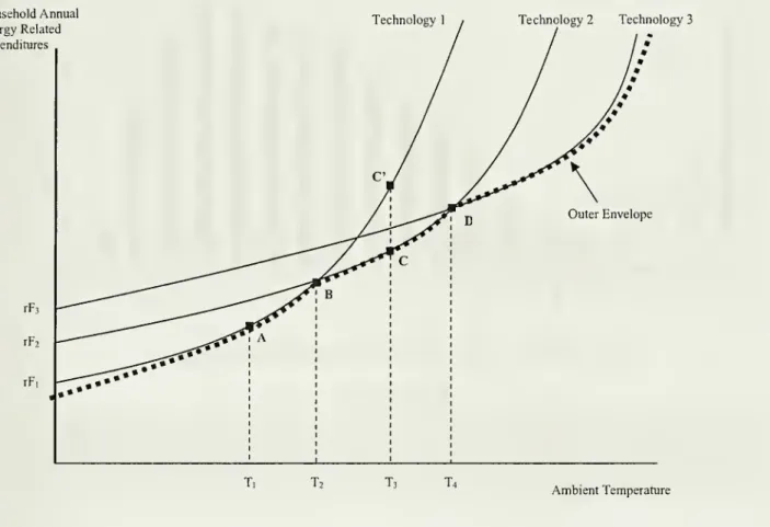
approachfailstocapturethese adaptations.

Figure 1 illustrates this issue inthe context ofalternative technologiesto achieve a given indoor temperature.

Household

annual energy related expenditures are on the y-axis and the ambient

temperature is

on

the x-axis. For simplicity,

we

assume

that an annual realization of temperature can be

summarized

in a single

number,

T.

The

figure depicts the cost functions associatedwith three different

technologies.

These

cost functions all have the

form

Cj

=

rFj

+

fj(T),

where

C

is annual energy related

expenditures,

F

is the capital cost ofthe technology, r is the costofcapital,

and

f(T) is the marginal cost

^ _{Energy consumption}

_may

_{affect utility through other channels in addition to} its role in self-protection. For example, high temperatures are uncomfortable. It would be straightforward toadd comfort to the utility function

and

make

comfort afunction of temperature and energy consumption. In this case, this paper's empirical exercise

would

fail to capture the impact of temperature on heat but the observed change in energy consumption would reflectitsrole inself-protection andcomfort.

which

is a function of temperature, T.

The

j subscripts index the technology.''

As

the figure

demonstrates, the cost functions differ in their fixed costs,

which

determine

where

they intersect the

y-axis,

and

theirmarginalcost functions or

how

costsrisewithtemperature.

The

cost minimizing technology varies with expectations about temperature. For example,

Technology

1 minimizescosts

between

Ti

and

Tt

and

the costs associated withTechnologies 1

and

2 are

identical at T2

where

the costfunctions cross (i.e., point B),

and

Technology

2 is optimal attemperatures

between

T?

and

T4.

The

outerenvelope ofleastcosttechnology choices isdepictedas thebrokenline

and

this is

where

households will choose to locate.^ Notably, there aren't

any

theoretical restrictions on the outerenvelopeasitisdetermined

by

technologiessoitcouldbe convex, linear, orconcave.

The

available datasets provide information on annual energy

consumption

quantities but not on

annual energyexpenditures. This

means

that existingdata sources can only identify the part ofthe cost

function associatedwiththemarginalcostsofambient temperatures orf(T). Further, ithighlightsthatthe estimation ofthe outerenvelope with data

on

quantities can reveal the equilibrium relationship

between

energy

consumption and

temperature.

However,

it is not informative about

how

total energy related

expenditures vaiy with temperature, precisely because the fixed costs associated different technologies

are unobserved.

One

clearimplicationis thatitis infeasibletodeterminethe impactofclimate

change

on

total energy expenditures with cross-sectional data as is claimed

by Mansur, Mendelsohn,

and Morrison

(2007).

We

now

discuss

what

can be learned

from

inter-annual variation in temperature andapanel data file

on

residential energy

consumption

quantities. Consider, an unexpectedincreaseintemperatures

from

Tito T3 for asingleyear,

assuming

thatit is infeasibleforhouseholdsto switch technologies inresponse.

The

representativehousehold's annual energy relatedexpenditures

would

increase

from

A

to

C

and

with fixed prices this is entirely captured

by

the increase in energy

consumption

quandties. Ifthe change in

'_{For illustrative purposes, consider the technologiesto becentral air conditioningwithout theuse ofinsulation in}

theconstructionofthehouse(Technology 1), central airconditioningwith insulation (Technology2),andzonal air

conditioningwithinsulation(Technology3).

^

_To

_{keep this example}

simple,

we

assume that there isn't any variation in temperature across years (i.e., the

expected standarddeviationof temperature ata locationiszero)and households basetheirtechnologychoiceonthis

information. In reality, technology choice depends on the full probability distribution ftinction of ambient

temperaturesatahouse'slocation.

temperature

were permanent

as

would

bethe case with climatechange, thenthe household

would

switch

to

Technology

2

and

their annual energy related expenditures

would

increase

from

A

to

C

(again this

cannot

be

inferred

from

data

on

energy

consumption

quantities alone). Thus,the

change

in

energy

related

costs inresponseto a single year'stemperature realizationoverstatesthe increase inenergy costs, relative

tothe

change

associatedwith a

permanent

temperatureincrease. It is

noteworthy

thatthe

changes

in costs associated with a

new

temperature

>

T|

and <

T2 are equal regardless of

whether

it is transitory or

permanent,becausethe outerenvelope

and Technology

1 costcurve areidenticaloverthisrange.

To

summarize,

this sectionhas derived an expression for

WTP/WTA

for climate

change

thatcan be estimated with available datasets.

The

first subsectionpointed out that

due

todatalimitations,

we

can

only

examine

a subset of the

outcomes

likely to be affected

by

climate change, so this will cause the subsequent analysis to underestimate the health-related welfare costs.

On

the other hand, the

second

subsection highlighted that our empirical strategy of utilizing inter-annual variation in

weather

will

overestimate the

measurable

health-related welfare costs, relative to the costs

due

to

permanent

changes

in temperature (unless the degree ofclimate

change

is "small"). This is because the available set of adaptations inresponsetoayear's weatherrealization isconstrained.

III.

Data

Sources

and

Summary

Statistics

To

implement

the analysis,

we

collected the

most

detailed

and

comprehensive

data available

on

mortality, energy consumption, weather,

and

predicted climate change. This section describesthese data

and

reports

some

summary

statistics.

A.

Data

Sources

Mortality

and

Population Data.

The

mortality datais taken

from

the

Compressed

Mortality Files

(CMF)

compiled

by

theNationalCenterforHealth Statistics.

The

CMF

contains theuniverse ofthe 72.3 million deaths in the

US

from

1968to 2002. Importantly, the

CMF

reportsdeath counts

by

race, sex, age group, county ofresidence, cause ofdeath,

and

year of death. In addition, the

CMF

files also contain population totalsforeachcell,

which

we

usetocalculate all-cause

and

cause-specific mortalityrates.

Our

sample

consists ofalldeathsoccurring inthe continental

48

statesplusthe Districtof Columbia.

Energy

Data.

The

energy

consumption

data

comes

directly

from

the

Energy

Information

Administration (EIA)State

Energy Data

System.

These

dataprovidestate-levelinformation about energy

price,expenditures,

and

consumption

fi'om 1968to2002.

The

datais disaggregated

by

energy source

and

end

usesector. Allenergydatais giveninBritish

Thermal

Units,or

BTU.

We

usedthe databaseto createan aimual state-level panel datafile for total energy

consumption

by

the residential sector,

which

is defined as"living quarters forprivate households."

The

database also

reports on energy

consumption by

the commercial, industrial, and transportation sectors.

These

sectors are not a focus ofthe analysis, because they don't

map

well into the health production function

model

outlined in Section II. Further, factors besides temperature are likely to be the primary determinant of

consumption

inthesesectors.

The

measure

of total residential energy consimiption is comprised of

two

pieces: "primary"

consumption,

which

is the actual energy

consumed by

households,

and

"electrical

system

energy losses."

The

latteraccounts forabout 2/3 oftotalresidential energy consumption; it is largely

due

to losses inthe

conversion of heat energy into mechanical energy to turn electric generators, but transmission

and

distribution andthe operation ofplants also account for part ofthe loss. In the

1968-2002

period, total

residentialenergy

consumption

increased

from

7.3quadrillion (quads)Britishthermalunitsto21.2quads,

and

the

mean

overthe entireperiod

was

16.6quads.

Weather

Data.

The

weather data are

drawn

from

the National

CHmatic Data

Center

(NCDC)

Summary

ofthe

Day

Data

(File

TD-3200).

The key

variables forouranalysis arethe daily

maximum

and

minimum

temperature as well as the total daily precipitation.^

To

ensure the accuracy ofthe weather

readings,

we

developed a weather station selection rule. Specifically,

we

dropped

all weatherstations at elevations

above

7,000 feet sincethey

were

unlikelyto reflect theweatherexperienced

by

themajority of

the population within a county.

Among

the remaining stations,

_we

considered a year's readings valid if

Otheraspectsofdailyweathersuchashumidity andwindspeed couldinfluence mortality,bothindividuallyandin conjunction with temperature. Importantlyfor our purposes,there is little evidencethat wind chill factors (a non-linearcombination of temperatureandwindspeed)performbetterthansimple temperaturelevelsinexplaining daily

mortalityrates(Kunstetal. 1994).

the station operated at least

363

days.

The

average annual

number

of stations with valid data in this

period

was

3,879

and

a total of 7,380 stations\met our

sample

selection rule for atleast

one

year during

the

1968-2002

period.

The

acceptable station-level datais then aggregatedatthe county level

by

taking

the simple average ofthe

measurements from

all stations within a county.

The

county

by

years with acceptableweatherdataaccountedfor53.4ofthe 72.3 milliondeaths inthe

US

from

1968to2002.

Climate

Change

Prediction Data. Climate predictions are based

on

two

state ofthe art global

climate models.

The

first is the

Hadley

Centre's 3rd

Coupled Ocean-Atmosphere

General Circulation

Model, which

we

refer to as

Hadley

3 (T. C. Johns et al. 1997,

Pope

et al. 2000). This is the

most

complex and

recent

model

in use

by

the

Hadley

Centre. It is a coupled atmospheric-ocean general

circulation model, so it considers the interplay ofseveral earth systems

and

is therefore considered the

most

appropriate for climate predictions.

We

also use predictions

from

the National Center for

Atmospheric

Research's

Community

Climate

System

Model

(CCSM)

3,

which

is another coupled

atmospheric-ocean general circulation

model

(NCAR

2007).

The

results

from

both

models were

used in the

4*

IPCC

report

(IPCC

2007).

Predictions of climate

change from

both of these

models

are available for several emission

scenarios, corresponding to 'storylines' describing the

way

the

world

(population, economies, etc.)

may

develop over the next 100 years.

We

focus

on

two

"business-as-usual" scenarios,

which

are the proper scenariostoconsider

when

judgingpolicies torestrict greenhouse gasemissions.

We

emphasize

the results

based

on predictions

from

the application ofthe

AlFl

scenario to the

Hadley

3 model. This scenario

assumes

rapid

economic growth

(including

convergence

between

rich

and

poor

countries)

and

acontinued

heavy

reliance

on

fossil fuels.

Given

the abundant supply of inexpensive

coal

and

otherfossil fuels, a switch toalternative sources is unlikelywithout greenhouse gas taxes or the equivalent, so this is a reasonable

benchmark

scenario. This scenario

assumes

the highest rate of

greenhouse

gasemissions,

and

we

emphasize

ittoexplore aworstcase outcome.

We

also present results

from

the application ofthe

A2

scenario to the

CCSM

3. This scenario

assumes

slower per capita

income growth

but largerpopulation growth. Here, there is lesstrade

among

nations

and

the ftiel

mix

is deteiTnined primarily

by

local resource availability. This scenario is

characterized as

emphasizing

regionaHsm

over globalization and

economic

development

over environmentalism. It is "middle ofthe road" interms ofgreenhouse gas emissions, but it

would

still be

consideredbusiness as usual,because itdoesn'tappearto reflectpolicies to restrictemissions.'

We

use the resultsofthe applicationof

AlFl

scenarioto the

Hadley

3

model and

the

A2

scenario

to the

CCSM

3

model

to obtain daily temperature predictions for the period

2070-2099

at grid points throughoutthe

US.

Each

setofpredictions isbased

on

a singlerunofthe relevantmodel.

The Hadley

3

predictions areavailable forgrid pointsspacedat 2.5° (latitude) x 3.75° (longitude),and

we

use the89 (of

the 153)gridpoints locatedon landtodevelopthe regional estimates. Sixstates

do

nothavea gridpoint,

so

we

developeddaily

Census

division-levelpredictionsforthe 9

US

Census

divisions.

The

CCSM

3 predictions are available ata finer level with separatepredictions available forgrid points spacedat roughly 1.4° (latitude) x 1.4° (longitude). Thereare atotal of

416

gridpoints

on

land in

the

US,

and

we

use

them

to develop state-specific estimates ofclimate

change

forthe years 2070-2099.

The

daily

mean

temperature

was

available forthese predictions,whereas the

minimum

and

maximum

are

available for the

Hadley

3 predictions.

The Data

Appendix

provides

more

details

on

theclimate

change

predictions.

B.

Summaiy

Statistics

MortalityStatistics. Table 1 reports the average annual mortality ratesper 100,000

by

agegroup

and

gender usingthe

1968-2002

CMF

data. Itis reportedseparatelyforall causesof death

and

fordeaths

due

to cardiovascular disease,

neoplasms

(i.e., cancers), respiratory disease,

and

motor-vehicle accidents

(since it is the leading cause ofdeath for individuals aged 15-24).'°

These

four categories account for roughly

72%

ofallfatalities,thoughtherelativeimportance of each causevaries

by

sexandage.

The

all cause

and

all age mortality rates for

women

and

men

are 804.4

and

939.2 per 100,000,

respectively, but there is

tremendous

heterogeneity in mortality rates across age

and

gendergroups. For

'

We

_{planned to have}

_AlFl

_and

_A2

_{predictions for both Hadley 3 and}

_{NCAR CCSM}

3, but

we

were unable to

obtain

AlFl

predictionsfor

NCAR CCSM

3and

A2

predictionsforHadley3.

'"in terms of ICD-9 Codes, the causes ofdeaths are defined as follows: Neoplasms

=

140-239, Cardiovascular Diseases

=

390-459, Respiratory Diseases

=

460-519,andMotorVehicleAccidents

=

E810-E819.

all-cause mortality, thefemale

and male

infantmortalityratesare 1,031.1

and

1,292.1. Afterthe firstyear

oflife, mortalityratesdon't

approach

this levelagain untilthe

55-64

category.

The

annual mortalityrate

startstoincrease dramatically atolder ages,

and

inthe75-99 age category itis

8.0%

for

women

and

9.4%

for

men.

The

higher annual fatality rates for

men

at all ages are striiiing

and

explain their shorter life expectancy.

As

is well-known, mortality

due

to cardiovascular disease is the single

most

important cause of

death in the population as a whole.

The

entries indicate that cardiovascular disease is responsible for

48.4%

and

43.6%

ofoverall female

and

male

mortality. It is noteworthy that the importance of the

different causes of death varies dramaticallyacrossage categories. For example,

motor

vehicle accidents account for

22.1%

(23.8%) of all mortality for

women

(men)

in the 15-24 age group. In contrast,

cardiovascular disease accounts for

59.6%

(53.7%) of all mortality for

women

(men)

in the 75-99

category,while

motor

vehicleaccidents are a negligible fraction.

More

generally, forthepopulation

aged

55

and

above—

where

mortality rates are

highest—

cardiovascular disease

and

neoplasms

are the

two

primary causes ofmortality.

Weather

and

Climate

Change

Statistics.

We

take advantage oftherichness ofdaily weatherdata

and

climate

change

predictions data

by

using the information

on

daily

minimum

and

maximum

temperatures. Specifically,

we

calculate the daily

mean

temperatures at each

weather

station as the

average

of

each day's

minimum

and

maximum

temperature.

The

county-wide

mean

isthencalculated as

the

unweighted

average across allstationswithina county.

The

climate

change

predictions are calculated analogously, except that

we

take the average ofthe daily predicted

mean

temperature across the grid

pointswithinthe

Census

Division

(Hadley

3)

and

state

(CCSM

3).

Table 2 reports

on

national

and

regional

measures

ofobserved temperatures

from 1968-2002 and

predicted temperatures

from 2070-2099.

For the observed temperatures, this is calculated across all

county

by

year observations with

nonmissing

weather data,

where

the weight is the population

between

ages

and

99.

The

predicted temperatures under climate

change

are calculated across the 2070-2099,

where

the weight is the population ofindividuals to 99 residing in counties with

nonmissing

weather

data inthe relevantgeographic unit

summed

overtheyears 1968-2002. It is importantto

emphasize

that

these calculationsofactualandpredictedtemperatures

depend

onthe distributionofthepopulationacross the

US,

so systematic migration (e.g.,

from

South to North)

would change

these

numbers even

without any

change

in theunderlying climate.

The

"Actual"

column

of Table 2 reportsthat the averagedaily

mean

is 56.6° F."

The

entries for

the four

Census

regions confirm that the South is the hottest part of the country and the

Midwest

and Northeast are the coldest ones.'^ Since people are

more

familiar with daily highs

and

lows

from

newscasts, the table also

documents

the average daily

maximum

and

minimums.'^

The

average daily spreadintemperatures is21.2°F, indicatingthathighsand lows candiffersubstantially

from

the

mean.

Figure 2 depicts the variation in the

measures

of temperature across

20

temperature bins in the

1968-2002

period.

The

leftmostbin

measures

the

number

ofdays with a

mean

temperature less than0°

F

andthe rightmostbin is the

number

ofdays

where

the

mean

exceeds 90° F.

The

intervening 18 bins are

all 5°

F

wide.

These

20

bins are used throughoutthe remainder ofthe paper, as they

form

the basis for

our semi-parametric

modeling

of temperature in equations for mortality rates and energy consumption.

Thisbinningofthe datapresei-vesthe daily variation intemperatures.

The

preservationofthis variationis

an

improvement

over the previous research

on

the mortality impacts of climate change that obscures

much

ofthe variation in temperature.''* This is importantbecause there are substantial nonlinearities in

the daily temperature-mortality

and

dailytemperature-energy

demand

relationships.

The

figure depicts the

mean number

of daysthatthetypicalperson experiencesineachbin; this is

calculated as the weighted average across county by year realizations,

where

the county

by

year's

population is the weight.

The

average

number

of daysinthe

modal

binof 70° - 75°

F

is38.2.

The

mean

" _{Theaveragedaily}

_mean

_{and allother entries inthetable (aswell as in theremainder ofthepaper) are calculated}

acrosscountiesthatmeettheweatherstationsampleselectionruledescribedabove,

'^

The

states in each ofthe Census regions are: Northeast— Connecticut, Maine, Massachusetts,

New

Hampshire, Vermont,

Rhode

Island,

New

Jersey,

New

York, and Pennsylvania;

Midwest—

Illinois, Indiana, Michigan, Ohio, Wisconsin, Iowa, Kansas, Minnesota, Missouri, Nebraska, North Dakota, and South Dakota; South— Delaware, District of Columbia, Florida, Georgia, Maryland, North Carolina, South Carolina, Virginia, West Virginia,

Alabama, Kentucky, Mississippi, Tennessee, Arkansas, Louisiana, Oklahoma, and Texas; and

West—

Arizona, Colorado, Idaho, Montana, Nevada,

New

Mexico, Utah,

Wyoming,

Alaska, California, Hawaii, Oregon, and Washington.

''^

Forcountieswithmultipleweatherstations, thedaily

maximum

and

minimum

arecalculatedastheaverageacross

the

maximums

andminimums,respectively,fromeachstation.

'"*

Forexample. Martens (1998) and Tol (2002a) use the

maximum

andthe

minimum

of monthly

mean

temperatures overthecourseoftheyear.

number

of daysattheendpoints is0.8forthelessthan0°

_F

bin

and

1.6forthegreaterthan 90°

F

bin.

The

remaining

columns

ofTable 2 report

on

the predicted changes in temperature

from

the

two

sets of climate

change

predictions for the

2070-2099

period.'^

The

CCSM

3

model

and

A2

scenario predict a

change

in

mean

temperature of 5.6°

F

or 4.1° Celsius (C). Interestingly, there is substantial

heterogeneity, with

mean

temperaturesexpectedto increase

by

9.8°

F

inthe

Midwest

and

by

3.0°

F

inthe West.

The

AlFl

scenario predicts a gain in

mean

temperature of6.0 °

_F

_{or 4.3° C.}

_The

_{increasesinthe}

Midwest

and

South

exceed

9°F, whilethereisvirtually

no

predicted

change

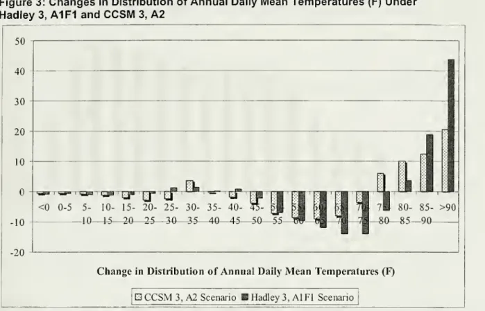
intheWest.'^

Figure 3 provides an opportunity to understand

how

the full distributions of

mean

temperatures

are expected to change.

One's

eye isnaturally

drawn

tothe last

two

bins.

The

Hadley

3

AlFl

(CCSM

3

A2)

predictions indicatethattypicalpersonwill experience 18.9 (12.4) additionaldays peryear

where

the

mean

daily temperature is

between

85°

F

and

90° F.

Even more

amazing,the

mean

daily temperature is

predictedtoexceed 90°

F

43.8 (20.7) extra days peryear.'''

To

putthis inperspective, theaverage person

currentlyexperiencesjust 1.6 days per year

where

the

mean

exceeds 90°

F and

7.1 inthe 85°- 90°

_F

_bin.

An

examination oftherest ofthe figure highlightsthatthe increase in thesevery hot days is not being

drawn from

theentireyear. For example,the

number

of days

where

the

maximum

isexpectedtobe

between

50°

F

and 80°

F

declines

by

62.6 (30.4) days

under

Hadley

3

AlFl

(CCSM

A2). Further, the

mean

number

ofdays

where

the

minimum

temperature willbe

below

30°

F

is predictedtofall

by

just 3.8

(10.4) days. Thus,these predictions indicate that the reductioninextreme colddays is

much

smaller than the increase in extreme hot days.

As

will

become

evident, this will

have

a

profound

effect

on

the

estimatedimpacts of climate

change

onmortality

and

energy consumption.

ReturningtoTable 2, the

bottom

panel reports

on

temperatures fordays

when

the

mean

exceeds 90° F,which, as

was

evident in Figure 3, is an especially importantbin.

The

paper's econometric

model

'^

Forcomparability,

we

follow

much

ofthe previous literature on climate change and focus on the temperatures

predictedtoprevailattheendofthe century. '^

The

fourth andmost recent

IPCC

reportsummarizes the current state ofclimate changepredictions. Thisreport

says thatthe adoubling of carbon dioxideconcentrations is "likely" (definedas P

> 66%)

to leadto an increase of average surfacetemperatures in the range of2° to4.5°

C

witha best estimate of3°

C

(IPCC

4 2007). Thus, the

predictions in Table 2 are at the high end ofthe likely temperature range associated with a doubling ofcarbon

dioxideconcentrations. '^

Attheriskofinsulting the reader,

we

emphasizethata

mean

dailytemperature of 90°F isveryhot. Forexample,

adaywithahigh of100°F

would

needa

minimum

temperaturegreaterthan 80°Ftoqualify.

assumes

that the impact ofall days in this bin on mortality

and

energy

consumption

are constant. This assumption

may

be unattractive ifclimate change causes a large increase in temperature

among

days in

this bin.

On

the whole, the increase in

mean

temperatures

among

days in this bin is relatively modest, with predictedincreasesof2.4°

F

(CCSM

3

A2) and

4.3°

F

(Hadley3 AlFI). Consequently,

we

conclude

thathistoricaltemperatures canbe informative aboutthe impacts ofthe additionaldayspredictedtooccur

inthe

>

90°

F

bin.

IV.

Econometric

Strategy

This section describes the econometric

models

that

we

employ

to learn about the impact of

temperature

on

mortalityrates

and

residentialenergyconsumption.

A. Mortality Rates.

We

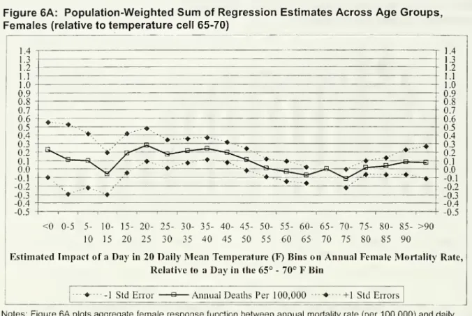
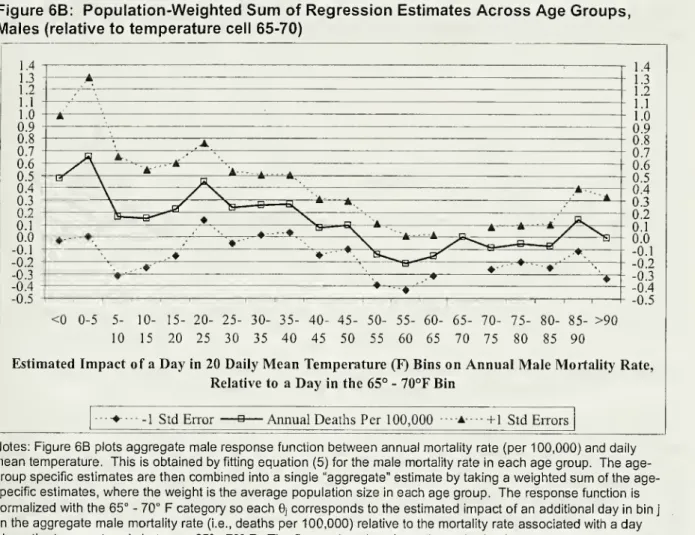
fitthe following equationsforcounty-level mortalityratesofvarious

demographic

groups:

J I

Ycidisthemortalityrate for

demographic

group dincountyc inyeart. Inthe subsequentanalysis,

we

use 16 separate

demographic

groups,

which

are

defmed by

the interaction of8 age categories (0-1, 1-14, 15-24, 25-44, 45-54, 55-64, 65-74,

and

75-I-)

and

gender. X^, is a vector of observable time varying

determinants offatalities

measured

at the county level.

The

last term in equation (5) is the stochastic

errortenn,s^,^

.

The

variables ofinterest are the

measures

of temperature andprecipitation,

and

we

havetried to

model

these variables with as

few

parametric assumptions as possible while still being able to

make

precise inferences. Specifically, they are constructedtocapture thefulldistributionof annual fluctuations

in weather.

The

variables

TMEANcj

denote the

number

of days in county c

and

year t

where

the daily

mean

temperature is in one of the

20

bins used in Figures 1

and

2. Thus, the only functional forai

restrictionis that the impact ofthe daily

mean

temperature is constant within

5F

degree intervals.'* This

'*_{Schlenkerand Roberts (2006)also}

consideramodelthatemphasizestheimportance ofnonlinearitiesin the

degree offlexibility

and

freedom from

parametric assumptions is only feasible because

we

are using 35

years of data

from

the entire

US.

Since

extreme

high

and low

temperatures drive

most

ofthe health

impacts of temperature,

we

tried to balance the dual

and

conflicting goals of allowing the

impact

of

temperature to vary at the extremes

and

estimating the impacts precisely

enough

so that they

have

empirical content.

The

variables PRECcti are simple indicator variables denoting annual precipitation

equalto"I" incountyc inyear.

These

intervalscorrespondto2 inchbins.

The

equationincludes a full set of county

by demographic group

fixed effects, a^j.

The

appeal

of including the county fixed effects is that they absorb all

unobserved

county-specific time invariant

determinants

of

the mortalityrate foreach

demographic

group. So,forexample, differences in

permanent

hospital quality or the overall healthiness of the local age-specific population will not

confound

the weather variables.

The

equation also includes state

by

year indicators, _y^^j, that are allowed to vary

across the

demographic

groups.

These

fixed effectscontrolfortime-varyingdifferences in the

dependent

variablethatare

common

within a

demographic group

inastate(e.g.,

changes

in state

Medicare

policies).

The

validityof any estimate

of

theimpact ofclimate

change based on

equation(5) rests crucially

on the

assumption

that its estimation will

produce

unbiased estimates ofthe

6.

and

S^i vectors.

The

consistency ofthe

components

of each

^

,.requires that after adjustment for the other covariates the

unobserved

determinants ofmortality

do

not covary withthe weather variables. In the case ofthe

mean

temperatures, this can be expressed formally as

E[TMEANctj

s^dI -^a> ^cd' Ystd]

~

0-

^y

conditioning

on the county

and

state

by

year fixed effects, the O^j's are identified

from

county-specific deviations in

weather about thecounty averages after controlling forshocks

common

to all counties in a state.

Due

to

the unpredictability of weather fluctuations, it

seems

reasonable to

presume

that this variation is

orthogonal to

unobserved

determinants

of

mortalityrates.

The

pointisthatthere is reasontobelieve that

the identification

assumption

isvalid.

A

primary motivation for this paper's approach is that it

may

offer an opportunity to identify

weather-induced

changes

inthe fatalityrate thatrepresent the full impact

on

the underlyingpopulation's

life expectancy.

Our

review oftheliterature suggeststhatthe full effectofparticularly hot

and

colddays

is evident within approximately 30 days

(Huynen

et al. 2001;

Deschenes

and

Moretti 2007).

Consequently, the results

from

the estimation of equation (5) that use the distribution oftheyear's daily temperatures shouldlargelybefreeofconcernsabout forward displacement

and

delayedimpacts. Thisis

because a given day's temperature is allowed to impact fatalities for a

minimum

of

30

days for fatalities

that occur

from

February through

December.

An

appealing feature of this set-up is that the Q™^^'^

coefficients can be interpretedas reflectingthe full long-runimpact ofaday with a

mean

temperature in

thatrange.

The

obvious limitation is thatthe weather inthe prior

December

(and perhaps earlier parts ofthe

yearifthe timeframeforharvestingand delayed impactsislonger than

30

days)

may

affectcurrentyeai-'s

mortality.

To

assess the importance ofthispossibility,

we

also estimate

models

that include afullset of temperature variables for the current year (as in equation (5))

and

the prior year.

As

we

demonstrate below, our approach appears to purge the estimates of fatalities of people with relatively short life

expectancies.'

There are

two

further issues about equation (5) that bearnoting. First, it is likely thatthe error

terms are con'elated within county by

demographic

groups over time. Consequently, the paper reports

standarderrors thatallowforheteroskedasticiy of anunspecified

form

and

thatare clustered atthe county

by demographic group

level.

Second, it

may

be appropriate to weight equation (5). Since the dependent variable is

demographic

group-specific mortality rates,

we

think there are

two complementary

reasonsto weight

by

the square root of

demographic

group's population (i.e., the denominator). First, the estimates of mortality rates with large populations will be

more

precise than the estimates

from

counties with small populations,

and

this weight corrects for the heteroskedasticity associated with the differences in

precision. Second, the results can then be interpreted as revealing the impact

on

the average person, ratherthan onthe averagecounty.

"

_A

_{daily version of equation}

(5) is very demanding ofthe data. In particular, there is a tension between our flexibility in modeling temperature and the

number

of previous days of temperature to include in the model. Equation (5) models temperature with 20 variables, so a model that includes 30 previous days would use 600

variables for temperature, while one with 365 days would require 7300 temperature variables. Further, daily

mortality data for the entire

US

is only available from 1972-1988, and there

may

be insufficient variation in

temperature within this relatively short period of time to precisely identify some ofthe very high and very low temperaturecategories.

Residential

Energy Consumption.

We

fit the followingequation for state-level residential energy consumption:

(6)

ln(C,

)

=

X

C'

TMEAN^

+

J^

5^'

PREC,

^XJ

+

a^+

y,,

+

s^,.

j I

Cs,is residential energy

consumption

in state s inyeartand d indexes

Census

Division.

The

modeling

of temperature

and

precipitation isidenticaltothe approachinequation (5).

The

onlydifference isthatthese

variables are

measured

at the state

by

year level

—

they are calculated as the

weighted

average ofthe county-level versions ofthe variables,

where

the weight is the county's population in the relevant year.

The

equationalso includes state fixed effects (

a^

)

and

census division

by

year fixed effects (7^,) anda

stochastic errorterm,

f

^,

.

A

challengeforthe successful estimationofthis equationisthattherehas

been

adramatic shiftin

the population

from

the North to the South over the last 35 years. Ifthe population shifts

were

equal

within

Census

divisions, this wouldn't

pose

a

problem

for estimation but this hasn't

been

the case. For example, Arizona's population has increased

by

223%

between 1968 and 2002 compared

tojust

124%

for

the otherstates in its

Census

Division,

and due

toitshigh temperatures itplays a disproportionaterole in

the identification ofthe dj 's associated withthe highest temperaturebins."°

The

point is that unless

we

correctly adjust for these population shifts, the estimated 0j 's

may

confound

the impact of higher

temperatureswiththepopulation shifts.

As

a potential solution to this issue, the vector X^^ includes the In of population

and

gross

domestic product

by

state as covariates.

The

latter is included since energy

consumption

is also a

function of income.

Adjustment

for these covariates is important to avoid

confounding

associated with

thepopulationshifts outoftheRust Belt

and

to

warmer

states.

Finally,

we

will alsoreport the results

from

versions of equation(6) that

model

temperature with

heating

and

cooling degree days.

We

followthe consensus

approach and

use abase of 65°

F

tocalculate

^^

Forexample,

we

estimated state byyearregressions forthe

number

ofdayswherethe

mean

temperaturewas in

the

>

90° Fbinthatadjustedfor statefixed effectsand census divisionbyyearfixedeffects.

The

mean

oftheannual

sum

ofthe absolute valueoftheresiduals forArizona is 3.6butonly0.6 in theotherstates in itsCensusDivision.

The other states in Arizona's Census Division are Colorado, Idaho,

New

Mexico, Montana, Utah, Nevada, and

Wyoming.