Design of innovative dynamic systems for seismic response mitigation

Design of Innovative Dynamic Systems

for Seismic Response Mitigation

by

Douglas Seymour

B.A., University of Cambridge, 2011

B.Sc., Canterbury Christ Church University, 2007

L BR RIES7

- h2V- -

--Submitted to the Department of Civil and Environmental Engineering in Partial Fulfillment of the Requirements for the Degree of

Master of Science in Civil and Environmental Engineering at the

MASSACHUSETTS INSTITUTE OF TECHNOLOGY

June 2012

@ 2012 Massachusetts Institute of Technology. All rights reserved.

Signature of Author

Dep _{and Environmental Engineering}

May 10, 2012

Certified by

Accepted by

/ Jerome J. Connor

Professor of Civil and Environmental Engineering The s Supervjsor

Heidi M. Nepf Chair, Departmental Committee for Graduate Students

ARCHIVES

Design of Innovative Dynamic Systems

for Seismic Response Mitigation

by

Douglas Seymour

Submitted to the Department of Civil and Environmental Engineering on May 10, 2012 in Partial Fulfillment of the Requirements for the Degree of Master of Science in Civil and Environmental Engineering

ABSTRACT

Rocking wall systems consist of shear walls, laterally connected to a building, that are moment-released in their strong plane. Their purpose is to mitigate seismic structural response by constraining a building primarily to a linear fundamental mode. This constraint prevents mid-story failure, and maximizes energy dissipation by activating the maximum number of plastic hinges throughout the structure. This is a useful response mitigation system, but suffers from some difficulties, stemming primarily from the considerable mass of the wall. Those difficulties are notably expensive foundations, and very high inertial forces imparted to the building, with subsequent need for expensive lateral connectors.

The purposes of this work are to analyze current implementations of rocking wall systems, present an early reference on their application, present the first systematic methodology for their design, clarify their analysis, and introduce an alternative structural system that avoids their difficulties. A quasi-static analysis model is used for predicting the seismic mitigation performance of rocking walls and rocking columns. The stiffness matrix is generalized for an N-story building equipped with these structural systems. The model presented enables optimization of the design parameters, and consequently improved system effectiveness, analytical tractability, and material usage. The case study is a rocking wall system installed in a building located in Tokyo, Japan. A software package is developed, providing an illustrative implementation of the methods derived.

Thesis Supervisor: Jerome J. Connor

Acknowledgments

I wish to give recognition to some of the many people who aided me in the completion of this

paper. First, to my advisor and friend Professor Jerry Connor, who taught me what it is to be a

civil engineer. Professor Connor suggested the topic, which is just one of a great many ideas that

he has helped me with. I would also like to thank my mechanical vibrations teacher and friend

Professor Eduardo Kausel for greatly advancing my understanding of vibrations.

I would also like to thank Professor Simon Laflamme, once Ph.D. candidate at MIT and now

professor at Iowa State University, for his help with the presentation of an earlier paper on this

topic, which aided my ability to produce a comprehensible academic paper tremendously. I

would also like to thank Professor Wada and Dr. Qu of the Tokyo Institute of Technology for

their assistance in providing data regarding the case study building. Professor Wada first sparked

my interest in rocking walls with a presentation he gave to Professor Connor's class in 2010, and

is presently the preeminent author in this field.

Contents

Page

1.

Introduction

11

1.1. Rocking Walls within the Taxonomy of Dynamic Structures

1.2. Outline and Purpose of Rocking Walls

1.3. Application of Rocking Walls 15

1.4. Outline History of Rocking Walls 16

2. Literature Review 18

2.1. Rocking Wall Design

2.1.1 Design for Resistance to Lateral Loads

2.1.2 Damping Design 19

2.1.3 Design for Serviceability

2.2. Lateral Load Bearing Capacity 20

2.3. Damping of Rocking Wall Systems 21

2.4. Ensuring Maximum Energy Dissipation with Linear 22

Deformations

2.5. Case Study: Retrofit of the G3 Building 23

2.5.1. Response of the Case Study Building to Seismic Loading 26

in the Transverse Direction

3.

Rocking Wall Design

28

3.1. Problem Statement

3.2. Method

3.4. Solving an Analytical Model without Rocking Wall 31

3.5. Solving an Analytical Model with Rigid Rocking Wall

3.6. Solving an Analytical Model with Flexible Wall, 33

Assumed Modes

3.7. Solving an Analytical Model with Flexible Wall, 34

Assumed Modes, Full Analysis

3.8. Applying Seismic Action to the Analytical Model 38

3.9. Applying Static Equivalent Seismic Action 39

3.10. Solving an Analytical Model with Flexible Wall, 42

with Full Stiffness Matrix

3.11 Benchmark Buildings 50

3.12. Software Implementation 52

3.13. Software to Implement ASCE 7-05 Equivalent Seismic 55 Loads

4. Analysis of Rocking Wall Design 57

4.1. Natural Frequencies of the Simulations

4.2. Natural Frequencies of the System With and Without 58

Rocking Wall

4.3. Modes of the System With Varying Stiffness of Rocking Wall

4.4. Maximum Story Drift Angle With Varying Rocking 60

Wall Width

4.5. _{Forces Applied to the Building by the Rocking Wall}

Inertia 62

4.6. Comparison with Given Case Study Building Data 64

5. Study to Determine Whether the Case Study Rocking

Wall Caused Damage During the Thhoku Earthquake 70

5.1. The Mathematical Model of the Building 71

5.2. Finite Element Modeling 72

5.4. Units and Consistency 77

5.5. Mass for Dynamic Analysis 78

5.6. Finding and Processing the Link Axial Forces in ADINA

5.7. The Addition of Damping to the Model 79

5.8. Calculation of the Static Shear Wall Cracking Moment 80

5.9. Conclusions of the Finite Element Study 81

6. Rocking Column Design 83

6.1. Rationale for Design

6.2. Introduction to Rocking Column Design 84

6.3. Further Rocking Column Design 86

6.4. Conclusions of the Finite Element Study 88

6.5. Conclusions of the Finite Element Study 89

6.6. Analysis of the Benefits of Rocking Columns 91

6.6.1 Lateral Force Reduction

6.6.2 Foundations Reduction 92

6.6.3 Cost Effective Connections

6.6.4 Greater Story Drift Reduction, with Potential for Further Reductions

6.6.5 Overall Comparative Effectiveness 93

7. Suggested Extensions 94

8. Conclusions 95

10. Appendices 101 Appendix A. The 20 Significant United States Earthquakes 1933-2006 103

Appendix B. A Set of Benchmark Building Models for Use 125 in Simulations

Appendix C. MATLAB Code for Solving the Rocking Wall as a 167

Flexible Continuous System, using Lagrange

Appendix D. MATLAB Code to Find the Stiffness Matrix of 171

1.

Introduction

1.1. Rocking Walls within the Taxonomy of Dynamic Structures

Dynamic structures avoid structural damage by shifting the burden of energy dissipation to chosen structural elements, preferably non-critical and replaceable elements. Damage that would result in severe injury, and damage that would prevent future serviceability of the structure, can be avoided by choosing the manner in which input energy is dissipated.

Dynamic Structures

F Linear Angular

Displacements Displacements

Base Isolation Rocking Walls

Figure 1.1.1. A partial taxonomy of dynamic structures

In addition to preventing loss of life, dynamic structures enable structures to be serviceable after a seismic event, and as such can be a highly sustainable approach to structural design in earthquake-prone regions.

1.2. _{Outline and Purpose of Rocking Walls}

A rocking wall is a dynamic structural system that employs one or more stiff structural elements,

moment-released at the base, to force a building that is subjected to dynamic loads to fail in a near-linear mode. This approach is intended to prevent mid-story failure, which is illustrated in figure 1.4.1, _{by maximizing energy dissipation, as discussed in section 2.4. As illustrated in}

figure 1.2.1, rocking walls are designed to rock only in the strong plane of the wall. This is in

strong contrast to a shear wall that is simply unrestrained at its base.

(a) (b) (C)

Figure 1.2.1. Schematic illustration of a simple unfixed shear wall contrasted with a rocking wall system. (a) Building with fixed shear wall, (b) Building with unfixed shear wall, (c) Building with rocking wall

All rocking walls have been constructed from reinforced concrete, as far as known at the time of

writing. As a result, the pin and foundations at the base of the wall must be highly substantial, as

illustrated in figure 2.1.2. Additionally, the lateral loads that the rocking wall imposes on the

surrounding structure during an earthquake are found, by an analytical method presented in this

work, to be very high partially due to the large mass of rocking wall, as discussed in section 4.5.

As a result, very substantial lateral supports are required to connect the rocking wall to the

building. All of these issues increase the cost of installation of a rocking wall system

substantially.

The Tokyo case study building, first introduced in section 2.5, was damaged in the

Tohoku earthquake of March 2011. Few buildings in Tokyo were significantly damaged in that

event, since as observed in Tokyo, the accelerations observed were one or two orders of

magnitude lower intensity than those observed nearer the epicenter. In section 5, a finite element

study is presented that supports the theory that the inertial loads from the rocking walls were

In response to these findings, it is suggested that new, higher lateral forces, as discussed in section 4.5, be considered when designing systems to be installed adjacent to rocking walls. Additionally, a much lighter steel system, resembling a deep column more than a wall, is proposed in sections 6-7. To differentiate the two systems, the new structural system will be referred to as a rocking column. Rocking columns achieve the goals of rocking walls at considerably less cost, by reducing the strength of additional foundations required, and the strength of lateral supporting connections that are required, in addition to material costs that are predicted to be significantly lower, making rocking columns more commercially viable than rocking walls have been.

Buildings that could be considered for rocking wall retrofit are in the approximate range 3 to 20 stories. The fundamental mode of such buildings is approximately linear.' As a result of this, the addition of a rocking wall adds a large mass but little stiffness to the fundamental mode. Thus it is clearly seen that the addition of a rocking wall will tend to decrease the frequency of the fundamental mode of the building, since frequency is inversely proportional to the root of mass. However, subsequent modes of such buildings are highly non-linear, as illustrated infigure 1.2.2, and thus a rocking wall adds a high stiffness to all other modes of the building, tending to increase those frequencies significantly, since frequency is proportional to the square root of the stiffness, and this effect is generally stronger than that of the mass in this situation. Thus for buildings that could be considered for rocking wall retrofit, the addition of a rocking wall tends to move all natural frequencies further away from the highest energy frequencies of earthquakes. This is clearly illustrated infigure 1.2.3.

Figure 1.2.2. A schematic of the first subsequent modes follow the same trend

three dynamic modes of a typical medium-height building. In general,

As figure 1.2.2 illustrates, general, exactly linear.

og20-CI18

-.

16

:14

-6

o2

₀

0.0

while the first mode of a building is often near linear, it is not, in

Frequency, Hz

2.0

4.0

6.0

8.0

Figure 1.2.3. Illustration showing how the application of a rocking wall system shifts the natural frequencies of a building away from the peak frequency range of earthquakes. The seismic data used to produce this figure may be found in Appendix A.

1.3. Application of Rocking Walls

For newly constructed buildings, there are many ways to prevent seismic damage, and a number

of ways to apply the benefits of dynamic structures. For example, the entire structural frame could be allowed to rock, with energy dissipation being performed by replaceable fuses, as

illustrated infigure 1.3.1. _{However, clearly for existing structures such a solution is not feasible,}

and other ways must be found to apply the benefits of dynamic structures.

Aroo~f

Post-Tensioning

Shear Fuse

Figure 1.3.1. A rocking frame structure.

Rocking wall retrofit projects are limited by the availability of appropriate locations to attach

rocking walls. Most often, such locations will be limited to the exterior of a building. In addition, for buildings that are large in plan, rocking walls must be spaced at some reasonable distance

throughout the building. Clearly, it is not sufficient to use rocking walls to linearize the response

of a building in one location alone. Rocking walls must be spaced throughout the building to

ensure the whole response of the building is linearized under dynamic loading. This approach

can be seen in the case study introduced in section 2.5, a building which is large in plan, and uses

As will also be seen from that case study, the building to be retrofitted was long and thin, and the

rocking walls were to be installed to the exterior, as would be most common, as illustrated in

figure 2.5.2. This meant that it was only appropriate to install rocking walls in the longitudinal

direction of the building, since if rocking walls were installed to the transverse direction of the

building, the center of the building in plan would be largely unsupported, since the distance

between rocking walls would be very large. This would result in the desired linearized transverse

mode for the thin edges of the building in plan, but the transverse mode for the center of the

building in plan would remain unlinearized.

In general, there is no particular problem with installing rocking walls in both orientations of a

building. But in the case study, although rocking walls were added to the longitudinal direction,

it was decided to stiffen the transverse response by adding conventional transverse shear walls, rather than add transverse rocking walls.

1.4. Outline History of Rocking Walls

The concept of rocking shear walls, though not in a form that matches current implementations,

was introduced by Ajrab et al.3 The work they presented was built on studies by Housner, who investigated the free vibration of rigid rocking blocks.4

Mander and Cheng defined an approach to rocking, structural flexibility, and prestressing, as

damage avoidance design.5 _{The performance objective of the DAD philosophy for a maximum}

assumed earthquake (MAE) is simply that the structure remains elastic at all times during ground

2 _{Deirlein (2010), p3}

shaking. For example, elastic rotations might be defined as rotations of less than 1%, 0.60.

Usually much less is preferred, for example the design criteria for the case study retrofit project

was a peak story drift angle of 1/250 radian (0.4% or 0.230)6. For a maximum considered

earthquake (MCE)7, the structure may yield with limited damage (for example defined as plastic

rotations of less than 0.5%) to the conventional reinforced concrete framing elements8. Rocking

can achieve these objectives, and are particularly relevant to retrofit applications.

Figure 1.4.1. Mid-story failure of Kobe city hallfrom the 1995 Kobe earthquake.

' Housner (1963) 5

Mander and Cheng (1997)

6 _{Wada (2010)(2), p}6 7 FE MA (1997), p32

8

2. Literature Review

2.1. Rocking Wall Design

The present work proposes that rocking walls are most appropriate for retrofit applications, due

to their relatively high cost and less than ideal architectural characteristics. However, earlier

papers on this subject considered that rocking walls would be applied to new buildings, and play

a significant role in the primary lateral load bearing capacity of the structure.

2.1.1. Design for Resistance to Lateral Loads

There are three central issues that have been considered in rocking wall design. The first is that

adequate resistance to lateral loads must be maintained. Since it was originally proposed that the

moment capacity at the base of walls be removed, this load bearing capacity must be transferred

to three other classes of mechanism, being the moment capacity of shear wall-to-frame

connections, the resistance to overturning of the weight of the wall itself, and to additional

mechanisms, such as bracing, or post-tensioned tendons running through the wall, which are

illustrated infigure 2.1.1. Pekcan et al. suggested that such tendons be draped to match the shape

of the moment diagram induced under the assumed inertial loading.9 Note that the original rocking wall concept presented is that of a flat base. If the rocking wall is pinned at the base, as

for example in the retrofit at the Tokyo Institute of Technology'0, then clearly the weight of the

wall itself offers no moment resistance.

.\ Rocking Too Lengthening _Apparent Shortening B'-B B=2b B-B B' B.

Figure 2.1.1. A non-hinged rocking wall on rigidfoundation, with supplemental supportive tendonsI(adaped)

2.1.2. Damping Design

Secondly, the rocking wall-supported structure must fulfil the primary intent of dynamic

structures by dissipating energy in a chosen, predictable way. Mander et al. conclude that a

tendon-supported rocking structure provides only limited damping, for example 1-2% of

critical. Percassi showed that the addition of damping devices to the tendons themselves would

enhance the damping offered by the system.'3

2.1.3. Design for Serviceability

The third central issue in rocking wall design, is the degree to which the structure is serviceable

following a seismic event. Kishiki & Wada discuss how following the Northridge and Kobe earthquakes, many buildings became structurally unviable, leading to a termination of social and

'0 Wada et al. (2009)

1Ajrab et al. (2004), p2

industrial activities, and consequently severe economic loss'4_{. A flat-based rocking wall as}

illustrated infigure 2.1.1 may suffer from toe crushing, and if rigid wall-frame connections are

used, these may also be significantly damaged. Such severe damage invariably requires that the

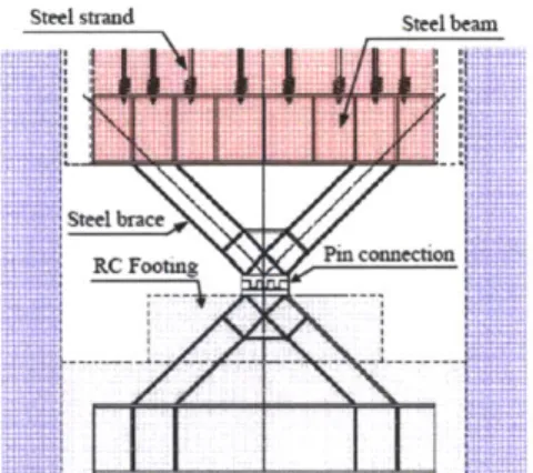
building be reconstructed, since further seismic performance cannot be predicted.5 _{An open pin}

design, fabricated from cast iron, at the base of the rocking wall would prevent severe damage to

the wall toes during rocking, as shown infigure 2.1.2.16

Steel strand Steel beam

3

RC Footmg Pmcneto

Figure 2.1.2. A rocking wall may be hinged at the base to prevent toe damage (foundations not shown)

2.2. Lateral Load Bearing Capacity

For a flat-based rocking wall on a rigid surface, and which is otherwise unsupported, it is readily

seen from statics that the lateral load that can be supported is:

W

Vax = (b - h) (2.1)

Heff(21

where W, is the weight of the wall, Heff is the point of application of the lateral load, b is half the

width of the wall, h is half the height of the wall, and 0 is the small angle through which the wall

has moved, as in figure 2.1.1.

13 Percassi (2000)

" Kishiki and Wada (2009), p1

' Wada et aL. (2009), p1

Further load-bearing capacity that may be derived is provided by the moment capacity of

floor-wall connections, and frame bracing. Example formulae providing the loading-bearing capacity

offered by floor-wall connections and supportive tendons are derived by Ajrab et al."

Of course in the case of a retrofit application of rocking walls, it will usually be reasonable to

assume that the existing structure has sufficient lateral load bearing capacity, except for seismic

loading, which is addressed as a special case by dynamic structures. All known applications of

rocking walls to date have been retrofit applications.

2.3. Damping of Rocking Wall Systems

The four sources of damping in a rocking wall-supported structure are inherent damping, which is typically taken to be 5% for concrete structures, radiation damping due to the impact of a

flat-based rocking wall with the ground, hysteretic damping due to plastic behavior within the frame, and supplemental damping such as dampers attached to the system. Formulae to illustrate

radiation damping and hysteretic damping are given by Ajrab et al.18

Various types of additional damping devices have been proposed, such as the fuse elements in

series with tendons proposed by Ajrab et al., and externally-mounted mild steel material dampers

proposed by Marriott et al.19 and implemented by Wada et al.2 0 _{Such devices may be installed}

with the intent that they be replaced after a seismic event.2 1

7 Ajrab et al. (2006), p2 1 Ajrab et al. (2006), _p3 1 Mariott et al. (2008), p2 20 _{Wada et al. (2009)} 2] _{Wada et al. (2009), p2}

2.4. _{Ensuring Maximum Energy Dissipation with Linear Deformations}

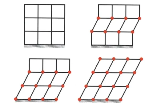
The introduction of rocking wall system to a frame building may be motivated by showing the benefit of a global failure mode with low rotations as opposed to a local failure mode with high rotations. Consider for example the simple frame with the three failure modes shown in figure 2.4.1.

Figure 2.4.1. (a) A schematic 3 story frame, (b), (c) its two non-ideal pushover failure modes, (d) its ideal pushover failure mode

It is readily seen that as the number of plastic hinges increases in the failure mode, so does the ability of the structure to dissipate energy. The first two failure modes shown have low energy dissipation, and so the rotations induced will be large, with high potential for loss of life and severe structural damage. However the final failure mode uses all possible plastic hinges, and thus has the maximum energy dissipation per unit rotation. Thus in this mode the rotations will be smaller, and the probability of saving life and further structural serviceability is maximized.

Hence the focus for seismic retrofit need not be strengthening the individual members which

would deform excessively under seismic loading, but rather the control of the global behaviour

of the structure to prevent damage from weak modes.

Additionally, it may be noted that the non-ideal failure modes are more likely to occur under

higher-mode excitation, since those forms are more congruent with the higher mode shapes, as

illustrated infigure 1.2.2.

Hence, if a rocking wall is designed to be rigid enough to resist the partial failure modes, the

frame will tend to fail in the preferable global failure mode. A rocking wall thus suppresses

higher mode vibrations,2 4 _{by moving the natural frequencies away from the peak energy range of}

earthquakes, as seen infigure 1.2.3.

2.5. Case Study: Retrofit of the G3 Building

To further understand the principles involved in the retrofit of a rocking wall, the retrofit of the

G3 Building at the Tokyo Institute of Technology, as discussed by Wada et al.,5 _{will be}

considered. The case study building was found to be inadequate for modem seismic codes, and

appropriate for retrofit. The design criteria for the retrofit project was a peak story drift angle of

1/250 radian (0.4%, 0.230), to prevent the shear failure of the reinforced concrete frame.26

23 _{Wada et al. (2009), p6}

24 _{Wada et al. (2009), pl0} 21 _{Wada et al. (2009)}

Figure 2.5.1. (a) The case study building in the Suzukakedai Campus of the Tokyo Institute of Technologyz,(aapted), (b) A 3D model of the retrofitted case study building, where yellow represents new structure to be retrofitted".

As is seen from figures 2.5.1(b) and 2.5.2, the design proposed by Wada et al. consists of wide

and shallow rocking walls (14.4ft by 2ft in plan) which rock in the longitudinal direction of the building. The rocking walls represent an additional 56% of the existing steel reinforced concrete

frame area, in plan. The wall is prestressed to allow for the large vertical tensile forces which

will result from inertial motion, and is designed to remain elastic during severe seismic motion.29

As is seen fromfigure 2.5.2, this retrofit only stiffens the response at six approximately evenly-distributed locations. The existing floor diaphragm stiffness between the rocking walls is

21 Wada (2010)(2)

intended to ensure that the response throughout the structure is close to the response at the

rocking walls themselves. The cross section-of a rocking wall is seen infigure 2.5.3.

Transverse Static Shear Wall

Rocking Wall _{Rocking Wall}

x

Figure 2.5.2. A plan view of the retrofitted case study building. Red represents rocking walls.30(adapied)

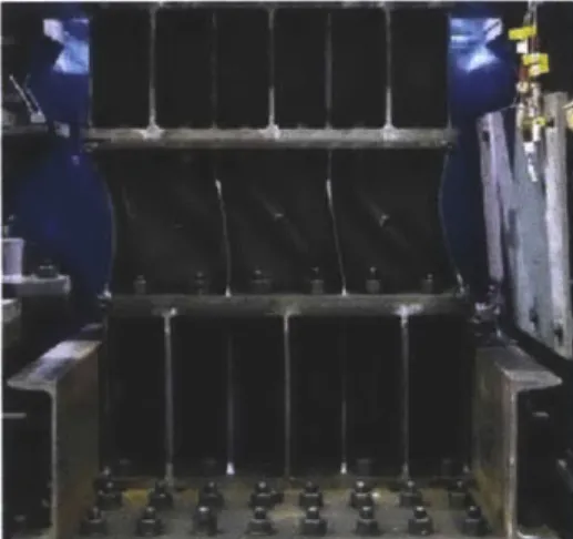
As shown infigure 2.5.3, the motion of the rocking walls in the case study building is damped by

the use of steel dampers (type LY22631_{), such as those shown in figure 2.5.4. These dampers}

reduce the story drift further than with the rocking walls alone. As discussed previously, the peak

story drift is already reduced by the rocking wall without any damping by equalizing the drift

burden throughout the structure.

Existing RC column Steel damper Rocking wall Steel strand -f P. .1 T, 7 374 T, i;1 M I 4 H a t 0 1

Figure 2.5.3. Cross-section of a rocking Wall. 32,adapledl

28 _{Wada et aL. (2009)}

21 _{Wada et al. (2009), p6-7}

Professor Wada's report on the case study retrofit concludes by discussing that the upper-bound

theorem is not easily applicable for a seismically controlled structure, which makes determining

the ultimate strength and seismic performance of the structure highly difficult.3 3

Figure 2.5.4. Testing of the steel dampers used in the case study retrofit project. 3 4

2.5.1. Response of the Case Study Building to Seismic Loading in the Transverse Direction

The report on the retrofit of the case study building indicates that both directions of the building

were below a seismic capacity of 0.7, and so were both required to be retrofitted. However the report does not directly mention the effects of the rocking wall retrofit on the response of the

building in the transverse y-direction, and only explicitly discusses the modeling of seismic

performance evaluation in the longitudinal x-direction 36. However, in a lecture, Professor Wada

3' Wada (2010), p7 32 _{Wada et al. (2009), p}7 3 Wada et al. (2009), p1 1 34 Qu and Wada (2011) 3s Wada et al. (2009), p5 36 _{Wada et al. (2009), p}8

mentioned the additional static shear walls which were added to the transverse direction3 7_{, and}

which are seen infigure 2.5.1. When a student asked about this issue, Professor Wada remarked

that the retrofitted building is adequately stiff in the transverse direction to resist severe damage,

and that the project is designed for 225% of the code requirements.38

3 Wada (2010)(2), p7 38 Wada _(2010)(1)

3. Rocking Wall Design

3.1. Problem Statement

Currently, each rocking wall design project requires an entirely new analysis from first

principles, with expert-level oversight. Such high design requirements are prohibitive in the

application of any new system. To aid in future maturation and acceptance of this structural

system, it is required to provide tools that systematize the selection of rocking wall properties,

based on the known parameters of the building to be retrofitted, to reduce the time required for

the analysis phase, and provide a framework for design. This will allow engineers to better

understand the structural system and aid discussion in this area of dynamic structures.

The most critical information to determine is the size of rocking wall that is required for a given

building. Secondly, it is required to determine the lateral loads that the rocking wall applies to

the building under code-determined seismic loading.

3.2. Method

In this work, the process of producing the tools alluded to in the problem statement is started

with the development of a number of analytical models of the rocking wall system, in sections

3.3 - 3.7 and 3.10.

A method is developed which may generate benchmark discretized buildings of any number of

stories, including story stiffnesses and story masses, such that the analytical model of the

Seismic loads are applied to the analytical model, and the responses of the model to those loads

are analyzed, as discussed in sections 3.8 - 3.9.

Example software is developed which implements those models programmatically, and returns

the required information, as discussed in sections 3.12 - 3.13.

3.3. Introduction to Analytical Model

For low- to medium-rise structures, which are the primary focus of retrofitting rocking walls,

buildings tend to deform approximately like a shear beam, under environmental loads. If the

building deformation were exactly linear, as shown in figure 3.3.1, then clearly a rocking wall

would add no stiffness to that particular deformation, only mass. In general this is close to the

truth for fundamental mode deformations. Although for all buildings with stiffness profiles that are not parabolic, there will be some non-linearity in the deformation under seismic loading.39

Figure 3.3.1. Low- to medium-rise buildings tend to deform like a shear beam

The principle of tributary areas can be used to model a low-rise building with an attached

rocking wall as shown infigure 3.3.2.

M2 u,,M2 -+- U2

k2 h k, h

MJ

{MJ

, U

j,--O-U

k1 h ki h

Figure 3.3.2. Schematic of a tributary two-story building model with rocking wall (a) without supplemental damping, (b) with supplemental damping

Initially, the rocking wall will be modeled as rigid. In subsequent models, the wall will be

modeled as having finite rigidity, with the intent that an optimum rigidity will be found that

maintains purely elastic deformation in the structure.

Initially, Lagrange's equation will be solved without taking the ground motion into account.

Assuming deflections are small, a condition which the rocking wall is intended to enforce, changes in gravitational potential energy may be neglected, and the stiffness of the columns may

be assumed to remain linear.

Three models of the rocking wall-building system are presented, of increasing complexity. First

a model with a rigid wall is presented, then a model with a flexible wall, and finally the complete

3.4. Solving an Analytical Model without Rocking Wall

Before the model including the effect of the rocking wall is solved, the model without the

rocking wall attached must be solved, so that the outputs of the two models can later be

compared and contrasted, and so the benefit that the rocking wall has introduced can be clearly

shown.

k, h

ki h

Figure 3.4.1. Lumped model of two-story building without rocking wall attached.

This system is of course trivial to solve,40 _{with a characteristic equation and fundamental}

frequency of:

[ 1

O1

[0 m 2 ji_2 [ - k2 k2 ju 2j

Col2= kI +k2 (.1b

=mi (3.b)

3.5. Solving an Analytical Model with Rigid Rocking Wall

The objective model is a model with ground motion, and flexible wall. But as a first model, the

ground motion, damping, and the flexibility of the wall can be ignored. The kinetic and potential

energies of the structure are thus:

K = %Amiu| + %1m2U

2

+ Y2MZI+ %J (3.2)

V = %k2u 2 + ki(u2

-

However, since the rocking wall is initially being modeled as rigid, and small rotations are

assumed, the geometric conditions exist:

u2= 2ui

=

and so without damping:

(3.4)

(3.5)

K = %Am ₁

u

+

V = %k2u, + % kul =(k, + k2)u = (mi + 4m2 + M+ -l l 0 -(ki + k2)ui Jv2 hI,)| J (3.6) (3.7) (3.8) (3.9) (3.10)

Thus from Lagrange's equation, the unforced equation of motion and natural frequency of the

structure are shown to be:

J

(mi + 4m2 + M+ )iI + (k, + k2)ui = 0 (3.11)

(3.12)

m, +4m2 + M + 2

h

Thus, assuming an approximately linear mode both with and without the rocking wall, the

rocking wall decreases the fundamental frequency by an amount equal to 1

M+

3.6 Solving an Analytical Model with Flexible Wall, Assumed Modes

This model is somewhat more realistic, but significantly more complex. In addition to a rigid

mode, an appropriate non-rigid mode shall be superposed. It is noted that the first non-rigid

mode and frequency of an ideal pin-ended beam free at the other end are:41

OD1 = (N) (3.17)

Q AL2

1sinh cxx ZRt 1 = sin c - asinh (L ere a= 4L

which, asfigure 3.6.1 shows, may be approximated as:

VI ~~-sin x

(3.18)

(3.19)

C1 CD sin

Figure 3.6. 1. The non-rigid trial mode (a) y,=sin ox - Isinh ox (b) Vi sin atc

Clearly, the rigid body mode is:

x

YO =T

Thus, if the following deformation form is assumed:

u = yloqo(t) + yiuqi(t)

(3.20)

(3.21)

Lagrange's equation may be applied to this problem, using the assumed modes method.

M2 -+- u' ,,mUp2,

kh h h

M, J m-u;'pA,L mI PI & P2. are

M, EI0 Pi ,, restorative forces

k h h from the building.

-+ ug ug

Figure 3.6.1. Further simplified rocking wall model

A model for the system may be presented as shown infigure 3.6.1. The building may be replaced by external restorative loads on the wall, which may be found by solving:

p=Kiu (3.22)

where Kb is the stiffness matrix of the building.

The method used to solve the above system is extensive, though programmatically relatively

straightforward. The MA TLAB code that was used to solve the above system using Lagrange's equations may be found in Appendix C.

3.7. Solving an Analytical Model with Flexible Wall, Assumed Modes, Full Analysis

A third method to apply the seismic action is to solve the continuous system problem using the

assumed modes method. This method requires a number of modes to be assumed, and increases in accuracy as the number of assumed modes is increased. This method is not subsequently used

in the final formulation presented in this work, but is included for completeness. This method is

similar to that presented in section 3.6, but does not simplify the problem by modelling the

In this formulation, two modes are considered: a linear mode /o, and a chosen mode y, for

which a good choice would be either of the modes shown in figure 3.6.1. In the following

derivation, u represents the absolute displacement and v the relative displacement to the ground.

Consider the general problem as shown infigure 3.7.1:

Akx k xa =aL m u x:t k X= cpL Ug _(t)

Figure 3.7.1. The rocking wall problem generalized

Fromfigure 3.7.1, it is observed that:

u(x,t)=v(x,t )+ug , i, ( =u(x,,,t)= u(aL,t), (3.23)

u, (t) = u(x,,t ) =u(8L,t) (3.24)

Now define:

K (aL) yj, , ,8L )= V1,,, (3.25)

then:

K -ILl2 k ₂ pAdx + _m'1d _2JuP1wTma +_jm Zd

2m16 13

{ (Q+d,)2

pAdx+m, (9,, + dg) + m,(9, +d, )2

(3.26)

=pA (L 4 +± , ++ , &)dx+m aaa4 + .4,+dg]mI 8[840 + Y,4, +d,

=PA x2dx + IIxdx+ fxdx +a2m+2m,) 4o (3.27)

+(ama + pm,y ₁0 ) 4 +(maa + mp)ii

= pA

(4

=pA x ₁ dx+ j dx+dL I Idx] + (aV,,ma + PIm)4 0 (3.28) +/2 Ma + iy1m, )4, +(VIama + yIflmf dg

Hence differentiate these to find:

d BK ( pAL+a2ma _+/2mp)ijo

dt 84 ₀ 3

(3.29)

+ jpA yxdx+a may,,a + /my₁, ij, + ({ pAL + maa + m,,p)fig

[±pA xy1dx+ayIma +fym, (

+[pA. dx+y2ma +V 2 mf 4 + pA, dx+yima+ym fig

Also:

V ={ Ev"2 d+k. (va -v_

_v2+

EI (vf) dx + ( -)2 ++ _(3.31) =

j

=k a a- 8)(a - )q O+

(

aqO (3.32)

av q

(3.33)

= [(a - -, V/)(yi y/i, )ka + PytIk, Iq0 + [EI N(yidx+(VIa _- Y, ₎2_{k, + Y2 k q,}

Finally, applying Lagrange's equations:

M + Kq = -muig

where:

=

ma +/J2

m

{±pA fx y1, dx +a Iama + 6VI,,,m,

IpA Vy,xdx+amaylia pA y / dx + y/ m, + Y/2 M +I#myiyf

J

(a -p8)(y/l -YI11)ka +py/,,pk,

Sp AL+maa+mp

M= , q= {qO (3.36)

pA yK, dx + y!,my/lfm, _qJ

Thus using the above formulation, the ground acceleration "g may be set to be the maximum ground acceleration Sa _{for a certain considered earthquake, and the system solved for that case.}

(a - p)r- yV 13) ka +8 Vy!,6k,

3.8. Applying Seismic Action to the Analytical Model

Applying seismic action to a model can be achieved a number of ways. To solve discrete

systems, the mass and stiffness matrices of the whole system M & K may be found, and the

system solved for an earthquake ground acceleration flg:4 2

MV+ Cv + Kv = -Meig (3.37)

where e is the unit constant rigid body vector, and v is the relative displacement:

v = u- eug (3.38)

However, in order to model the rocking wall, a continuous element, another approach must be

taken. One option is to discretize the rocking wall into lumped masses, and solve the problem as

a discrete dynamic system. The other is to solve the flexible wall problem fully analytically as in

section 3.7.

The quasi-static approach to applying seismic action is to apply forces, which are proportional to

the square of the height, to the masses of the building. The values of these forces may be found analytically, and guides to aid their calculation are found in building codes. To solve the rocking

wall as a statics problem, these loads may be applied to the analytical model, and find the

resultant displacements.

To achieve either of the above methods of applying the seismic action, the stiffness matrix for

the rocking wall-building system must be determined. This may be found empirically, for

example using a finite element approach for a specific system under consideration.43 _{However, it}

42 _{Chopra (2006)}

would be far more valuable to determine the general analytical stiffness matrix of this system, for any given system parameters. That stiffness matrix is derived in Section 3.10.

3.9. Applying Static Equivalent Seismic Action

There are various methods of force-based design and analysis, such as equivalent lateral force

method, response spectrum method, nonlinear static analysis, and nonlinear time-history

analysis. The equivalent lateral force method is valid for modeling linear systems in 2D and

considers the fundamental mode. This is particularly appropriate for the rocking wall-building

system, since the system is intentionally constrained to primarily fundamental mode action.

The equivalent lateral force method involves representing the seismic activity as forces applied

at each story by the equation:

Vh 2

Fj - = (3.39)

Y

where V is the base shearj, i are the floor number starting from the first floor above ground, h is

the height of the floor from ground, and m is the mass of the floor.

The procedure for determining the equivalent lateral forces follows.4 4

The seismic base shear V, is determined by:

V = CW _(3.4045)

where C, is the seismic response coefficient, and W is the effective seismic weight.

44

The effective seismic weight of the building W, is defined by the code.46_{Cs is given by:}

SW CS = SDS

(R)

47

where SDs is the design spectral response acceleration at short period, R is the response

modification factor, and I is the occupancy importance factor.

The design earthquake spectral response acceleration parameter at short period, SDS, is given by:

SDS MS

3 (3.42 48)

where SMs, the Maximum Considered Earthquake (MCE) spectral response acceleration for short

periods, is given by:

SMS = F.S, (3.4349)

Here, S, is the mapped MCE spectral response acceleration at short periods and Fa is a site

coefficient. Fa is dependent on the Site Class and Ss. Ss is determined from the 0.2s spectral

response accelerations as shown by a contour map of the Unites States given in a specified figure.

The code states that "Where the soil properties are not known in sufficient detail to determine the site class, Site Class D shall be used.".5 In that case, Fa is found to be 1.6.

4 sASCE (2006), Eqn. 12.8-1 4 6 ASCE (2006), Section 12.7.2 4 7 ASCE (2006), Eqn. 12.8-2 4 8 ASCE (2006), Eqn. 11.4-3 * ASCE (2006), Eqn. 11.4-1 5 0 ASCE (2006), Figure 22-1 si _{ASCE (2006), Section 20.1}

Assuming an Occupancy Category of j,53 the importance factor, I, is determined to be 1.25.

The response modification factor R is determined to be 4, assuming an ordinary reinforced

concrete shear wall.

The value of Cs must not exceed:

C, = SD1 TR) T C, = SDTL T 2(R I) for T !TL (3.4 5) for T >TL (3. 46'7)

Additionally, Cs must not be less than 0.01.58

For structures located where S, > 0.6g, C, must not be less than:

0.5S

C=C IJ (3.4 759)

(R)

In the above formulae, SDI, TL, T, and Si are to be evaluated.

SDI _{is the design earthquake spectral response acceleration parameter at Is period, and it is} determined by:

5

2 ASCE (2006), Table 11.4-1 5 3

ASCE (2006), Table 1-I

54 ASCE (2006), Table 11.5-1 "5 ASCE (2006), Table 12.2-1 5 6 ASCE (2006), Eqn. 12.8-3 5 7 ASCE (2006), Eqn. 12.8-4 5 8_{ASCE (2006), Eqn. 12.8-5} * ASCE (2006), Eqn. 12.8-6

SDI = 2S

3

SMI, the MCE spectral response acceleration at Is period, is determined by:

S, = F SI

(3.4860)

(3.4961) Si, the mapped MCE spectral response acceleration at a period of Is, is determined from a specified figure,62 _{and F,, a site coefficient, is determined from a specified table.}63

T is the fundamental period of the structure. The approximate period Ta

T, = C,h'n

where h, is the height in feet above the base to the highest level

coefficients C, and x are determined from a specified table.65

is found by the formula:

(3.5064)

of the structure and the

3.10. Solving an Analytical Model with Flexible Wall, with Full Stiffness Matrix

The full analytical model of the rocking wall-discretized building system, concluding with the definition of the general stiffness matrix for this system, is first derived in this section.

6 0 ASCE (2006), Eqn. 11.4-4 " ASCE (2006), Eqn. 11.4-2 62 ASCE (2006), Figure 22-2 63 ASCE (2006), Table 11.4-2 1 _{ASCE (2006), Eqn. 12.8-7}

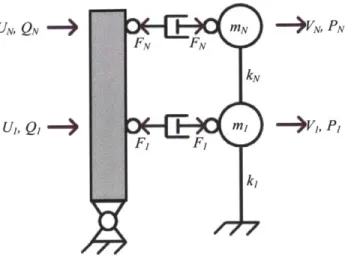
Figure 3.10.1. The statically condensed rocking wall-building system to be modeled.

The rocking wall-structure system is illustrated in figure 3.10.1, in which k, and m; represent the

stiffness and tributary mass respectively of the ith story. The development of the model begins by

representing the rocking wall as a hinged beam, as shown infigure 3.10.2, in which F; represent

any loading on the beam that is constrained to static equilibrium.

L

F₁ F2 FN

Figure 3.10.2. Model of the free rocking wall.

Computing moments about the pin, assuming constant inter-story height for simplicity, and

setting the lowermost force to be a function of the others, an expression to describe the link

forces Fi is obtained,

Fi = -2F2 - 3F3 ...- NFN (3.51)

6 5

These forces may be applied to the beam model in balanced pairs. First FN at node N with a

reaction of -NFN at position 1, illustrated in figure 3.10.3, followed by FN-1 at node N-1 with a

reaction of -(N-1)FN-1 at position 1, and so on.

NFN

h Ah FN

Figure 3.10.3. Loads applied to the mechanism in pairs, maintaining static equilibrium

It is shown readily that the order N-1 pseudo-flexibility matrix Ewaji consists of elements:

{Fwai = 3-x + 3a) (ij; 1 i,j N-1; i.e. xsa) (3.52) l~al)i=3NEf ± + 3a

aL a2

{Fwaiiaii = 3NEf ± (3X - a) (i>j; I :sij!N-1; i.e. x>a) (3.53)

which consist of a rotational term and a cantilever term, and where x and a are distance to point

of measurement and distance to point of application of load from the pin respectively, and

obtained as:

i-2

x = NL (3.54)

a = L (3.55)

Thus rather than providing the displacements, Fwall provides the relative shape,

W = F 11 F, of the wall, under the statically-balanced loading F, where the zero reference line

is projected from the pin, through the lowest load-position on the beam, as illustrated in figure

N

(W

(II

Figure 3.10.4. The model beam under an arbitrary loading and dejormation. The reference line, shown dashed, coincides with the lowest beam reference position, requiring that the relative displacement W1=0. yV is the small

angle through which the reference line is displaced.

A vector of displacements relative to the reference line may be defined as W. The total

displacement of the wall is given by _E, _{plus a rigid body rotation. For now, let W be of size N-1,}

omitting the lowest relative displacement W = 0. The analysis may be continued by recognizing that since the beam is a mechanism, it may be rotated to any arbitrary small angle V under an

arbitrary balanced loading, such that the absolute positions of the beam are a rigid body rotation

displacement j, plus the deviations from that line, _W. Additional information is required to fix the beam in space. Consider the model in figure 3.10.5, where U, V, P,

Q,

UN, QN -)

U, Q; -M -- V, P,

F, F,

Figure 3.10.5. The rocking wall-building system model with forces and displacements required to complete the analysis

From the previous discussion, a matrix Fwalu that uniquely maps the upper N-i net forces to the

relative displacements of the wall W is determined. Since this mapping is clearly unique, Fwau1 may be inverted to Kwan. Thus the order of Kwau may be incremented to N, by temporarily adding

a leftmost zero column and topmost zero row. Thus Kwau now uniquely maps all N relative

displacements _W, including the lowest relative displacement W, which is always zero, to the

upper N-I forces

E&'

Ew' = KwauW (3.56)

The vector

E'

the lowest position on the wall as zero. That force may be determined by applying moments at

the pin. A matrix M0 may be formulated which enforces the principle of moments, such that:

F,, 0 Ew- . -MaF' (3.57) 0 where: --)N, PN

0 (N -1) - N

MO =

-0 ... ... 0 _

Thus, the complete net force on the wall is found to be:

, = F,' + MoFw' = (Mo + I)F ,'= (Mo + I)KauW (3.59)

Since the total forces on the wall and on the building are defined as:

_F =Q-F Fb= P + F

(3.60) (3.61) These may be rearranged to:

F = Q -F, = Q - (Mo + I)KwaW (3.62)

(3.63)

F=Eb- P = KbIdg_ - P

Applying Newton's third axiom, the above two formulae may be equated and rearranged:

KbIdgU + (Mo + I)KwaiW = P +

Q

As discussed, the absolute displacement of the wall is given as:

V= g+ W (3.65)

where _ is the arbitrary rigid body rotation vector, and W is the relative displacement of each

point about that rigid body rotation. If V is the scalar angle of rotation, then:

h 2h

Nh]

(3.66)

And since the lowest position lies on the line by definition:

Vy

Thus equation 3.65 becomes:

V=

V12l

-N_ or:

LV (3.69)

where L1 is a linear matrix that acts on the 1st term of a vector:

1 0 ... 0~

L,=2 (3.70)

_N 0 ... 0_

Substituting equation 3.69 into equation 3.65, it is found that:

WE= V-LV=(I-L 1)_ (3.71)

which may be substituted into equation 3.64 to yield:

KbldgU + (Mo + I)Kwaii(I - L,)V = P +

Q

If damping is to be added between the wall and the building, U and V must be considered

independent. However, damping is outside of the scope of this work, where only quasi-static

loading is considered. Without damping, it may be assumed that the links are rigid, and thus that

the building displacements U are equal to the wall displacements V. Thus the stiffness matrix of the undamped system is finally shown:

where P +

Q

Using the displacements U found with equation 3.73, equation 3.61 may be rearranged to find F,

the forces in the links:

F=Eb- P = KbidgP (3.74)

If a structure makes use of supplemental damping systems, and the seismic loads are to be

applied in a quasi-static fashion, this measure of the link forces should be considered as an upper

bound, since that method of applying seismic loads implicitly discounts any supplemental damping that may be added to a system.

This general model matches a good linear finite element analysis exactly, as illustrated infigure

U1 =-.1087 U2- 0 U3= 0 R1 = 0 R2 = -.00315 R3= 0 U=[ 0.135317, % storeydrift(1) = 0.008104 0.127212; % storeydrilt(2) = 0.008741 0.118471; % storeydrif(3) = 0.009737 % storeydrmt(4) = 0.010852 0.097883; % storey,_drl(5) = 0.011935 0.085947; % storeydrifI(6) = 0.012900 0.073048; % storeydrift(7) = 0.013702 0.059346; % storeydrift(8) = 0.014325 0.045021: % storev driff(g) 0.014773

Figure 3.10.6 (a) & (b) A linear finite element model shown matching the analytical model derived above to every significant figure returned. In this case the structure is loaded under seismic equivalent loading.

3.11. Benchmark Buildings

In order to illustrate some of the ways in which the methods presented in this work may be

applied, it was required to develop a set of benchmark buildings, which could reasonably

represent buildings that might be found in practice. The benchmark buildings were to consist of

stiffness profiles, mass profiles, and varying numbers of stories.

This requirement is a common one for structural research, and yet to the best of my knowledge, no qualified set of benchmark buildings, or method for producing a qualified benchmark

building, is readily available to students and researchers.

As a significant sub-project of this work, a fully comprehensive method was developed, using

define benchmark buildings. Using that method, 56 benchmark buildings were developed,

ranging from 2 to 15 stories in height. These benchmark buildings were tested with 116 different

rocking wall configurations, and the rocking wall design graph, as shown in sections 4.4 - 4.6,

for each benchmark building was found.

The method of creating benchmark buildings, the data for the benchmark buildings generated,

and the associated rocking wall design graphs, may be found in Appendix B.

The intent of the tables in Appendix B is that an engineer implementing a rocking wall project

would be able to find a close approximation of the building under consideration, and in a matter

of minutes determine the approximate size and number of rocking' walls that would be

appropriate, and whether rocking wall retrofit would be appropriate at all.

It is seen from the tables, for example, that for the benchmark (and thus intended to be

representative) buildings of only two stories, there is no possible rocking wall configuration that will reduce the maximum story drift. And many other similarly interesting conclusions may also

be drawn from the tables.