Design and optimization of imaging systems by engineering the pupil function

Design and Optimization of Imaging Systems by

Engineering the Pupil Function

by

Saeed Bagheri

Submitted to the Department of Mechanical Engineering

in partial fulfillment of the requirements for the degree of

Doctor of Philosophy in Mechanical Engineering

at the

MASSACHUSETTS INSTITUTE OF TECHNOLOGY

@

Massachusetts Institute

May 2007

of Technology 2007. All rights reserved.

Author ...

Department of Mechanical Engineering

May 3, 2007

Certified by...

Daniela Pucci de Farias

Assistant Professor, Mechanical Engineering

Thesis Supervisor

A

... (..•;..

A 11

Accepted by...

...

."

"•allit

and

S·ait

Anand

Chairman, Department Committee on Graduate Students

MASSACHUSETTS INSTITUTE OF TECHNOLOGY

JUL 1

8

2007

-Design and Optimization of Imaging Systems by Engineering the Pupil

Function

by

Saeed Bagheri

Submitted to the Department of Mechanical Engineering on May 3, 2007, in partial fulfillment of the

requirements for the degree of

Doctor of Philosophy in Mechanical Engineering

Abstract

It is expected that the ability to accurately and efficiently design an imaging system for a specific application will be of increasing importance in the coming decades. Applications of imaging systems range from simple photography to advanced lithography machines. Perhaps the most important way to make an imaging system meet a particular purpose is to engineer the pupil function of the imaging system. This includes designing a pupil surface and often involves the simultaneous design of a post-processing algorithm. Currently these design processes are performed mostly by using numerical optimization methods. Numerical methods in general have many drawbacks including long processing time and no guarantee that one has reached the global optimum. We have developed analytical approaches in designing imaging systems by engineering the pupil function.

Two of the most important merit functions that are used for the analysis of imaging systems are the modulation transfer function (MTF) and the point spread function (PSF). These two functions are standard measures for evaluating the performance of an imaging system. Usually during the design process one finds the PSF or MTF for all the possible degrees of freedom and chooses the combination of parameters which best satisfies his/her goals in terms of PSF and MTF. In practice, however, evaluating these functions is computationally expensive; this makes the design and opti-mization problem hard. In particular, it is often impossible to guarantee that one has reached the global optimum.

In this PhD thesis, we have developed approximate analytical expressions for MTF and PSF of an imaging system. We have derived rigorous bounds on the accuracy of these expressions and established their fast convergence. We have also shown that these approximations not only reduce the calculation burden by several orders of magnitude, but also make the analytic optimization of imaging systems possible. We have studied the detailed properties of our approximations. For instance we have shown that the PSF approximation has a complexity which is independent of certain system parameters such as defocus. Our results also help in better understanding the behavior of imaging systems. In particular, using our results we have answered a fundamental question regarding the limit of extension of the depth of field in imaging systems by pupil function engineering. We have derived a theoretic bound and we have established that this bound does not change with change of phase of pupil function. We have also introduced the concept of conservation of spectral signal-to-noise ratio and discussed its implications in imaging systems.

Thesis Supervisor: Daniela Pucci de Farias Title: Assistant Professor, Mechanical Engineering

Acknowledgments

First, I would like to thank my adviser, Prof. Daniela Pucci de Farias. This work would not have been possible without her enthusiasm, guidance and generosity in allowing me to pursue my own ideas and research directions. I will forever be grateful to her for giving me increasing levels of responsibility as my graduate experience progressed. I would also like to thank my informal adviser, Prof. George Barbastathis. I am deeply indebted to him for being an enthusiastic and genius supervisor. His comments and insights were invaluable sources of support for me. I am also grateful to the other member of my thesis committee, Prof. Peter So for his insightful recommendations.

The research presented in this dissertation is a result of close collaboration with Prof. Mark A. Neifeld and Drs. Paulo E. X. Silveira, Ramkumar Narayanswamy and Edward Dowski. I would like to thank them all for their valuable comments and suggestions. Special thank goes to Paulo for his continuous support and encouragement and many hours of helpful discussion. I am also grateful to researchers in CDM Optics for two great summers in the research industry. Furthermore, I would like to thank Drs. Michael D. Stenner, Kehan Tian and Wenyang Sun for insightful discussions and exchange of ideas.

My education at MIT was enriched by interaction with fellow students and friends. I am es-pecially grateful to Angelina Aessopos, Mohammad-Reza Alam, Husain A. Al-Mohssen, Mohsen Bahramgiri, Lowell L. Baker, Reza Karimi, Hemanth Prakash, Judy Su, Dimitrios Tzeranis and Yunqing Ye for making the courses and research as well as life in MIT much more fruitful. I would like to also thank my other friends, namely Salman Abolfathe Beikidezfuli, Mohammad Araghchini, Mohammad Azmoon, Hoda Bidkhori, Megan Cooper, Eaman Eftekhary, Shaya Famini, Ali Fara-hanchi, Ghassan Fayad, Julia Greiner, MohammadTaghi Hajiaghayi, Fardad Hashemi, Ali Hosseini, Asadollah Kalantarian, Ali Khakifirooz, Danial Lashkari, Hamed Mamani, Vahab Mirrokni, Ali Parandehgheibi, Mohsen Razavi, Saeed Saremi, Ali Tabaei, Hadi Tavakoli Nia, Luke Waggoner and many others for creating a joyful and unforgettable three years for me. I am also grateful to the staff of Mechanical Engineering Department, specially Leslie Regan, Joan Kravit and Laura E. Kampas for providing a nice academic environment.

I would like to use this opportunity to thank my undergraduate advisers, Prof. Ali Amirfazli, Prof. Mikio Horie and Dr. Daiki Kamiya for shaping my career path. Also I am grateful to Seid Hossein Sadat, Hamidreza Alemohammad and Reza Hajiaghaee Khiabani for many helpful discussions.

I thank my family for their unconditional support throughout these years. They provided every-thing I needed to succeed. My parents' everlasting love and prayer has always been and will remain a primary source of support for me and I am forever indebted to them for that. I am grateful to my brother, Vahid for being out there for me and to my sister, Maryam for her love. Last but not least, I thank my wife, Mariam for her understanding, inspiration and endless love. This thesis is dedicated to my family.

Contents

1 Introduction and Overview 17

1.1 Pupil Function Engineering ... 17

1.2 Motivation ... 18

1.2.1 Computation Time Versus Accuracy ... .... 19

1.2.2 Analytical Optimizations ... 19 1.2.3 Physical Understanding ... 20 1.3 Background .... .... ... . .. . .... .. .. .. .. ... .. ... ... . 21 1.3.1 Numerical Results ... 21 1.3.2 Analytical Results ... 22 1.3.3 Depth of Field ... ... .. 22 1.4 Contribution ... .. 23

2 Modulation Transfer Function 25 2.1 Introduction ... ... .. 25

2.2 Analytic M TF ... 27

2.3 Optimization for Uniform Image Quality ... ... 33

2.3.1 Statement of the Problem ... 33

2.3.2 Optimization ... ... .. 35

2.3.3 Results ... ... . 38

2.4 Optimization for Task-based Imaging ... ... 41

2.4.1 Statement of the Problem ... ... 41

2.4.2 Optim ization ... ... .. 43

2.4.3 Results . . . 48

2.5 D iscussion . . . 54

3 Point Spread Function 59 3.1 Introduction .. . . ... . ... . .. . ... . ... .... .... ... .. .. .. 59

3.2 The Optical Point Spread Function ... 62

3.2.1 Schwarzschild's Aberration Coefficients ... ... 64

3.3 The PSF Expansion for Arbitrary Wavefront Errors and Defocus . ... 66

3.4 Exam ples . . . . 69

3.5 Complexity Analysis ... ... .. 72

3.6 Discussions ... ... .. 77

4 Depth of Field 81 4.1 Introduction ... ... 81

4.2 The Spectral Signal-to-Noise Ratio ... 83

4.3 The Ambiguity Function and the Modulation Transfer Function . ... 85

4.4 Conservation of the Spectral Signal-to-Noise Ratio . ... 87

4.5 D iscussion . . . . 90

4.5.1 Limit of Extension of Depth of Field ... .... 91

4.5.2 The Brightness Conservation Theorem ... ... 93

5 Conclusions 97

A Derivation of Eq. (2.1) 101

B The MTFal Approximation 105

D The Solution of Equation (2.12)

E MTF Approximation Properties

F Derivation of the Expansion for the Point Spread Function

G Derivation of the Sm nkN (3) in Equation (3.19) H Complexity Proofs 117 121 127 133 137

List of Figures

2-1 Schematic view of optical system under consideration. . ... 29 2-2 Plot of e (&, 4, u) as a function of & and u (Note that all variables are dimensionless). 31 2-3 Plot of IMTFa2 - MTFal as a function of & and u when W20 = 4 (Note that all

variables are dimensionless) ... 32

2-4 Photos of a non-planer object with (a) traditional imaging system and (b) imaging system with pupil function engineering. Part (a) does not have a uniform image quality. Quality is good at best focus in the center of the photo and image gets blurry out of focus. Part (b) has a uniform image quality; i.e. the image quality is the same both in and out of focus. Here by uniform image quality we mean the uniform transfer function of the imaging system at the spatial frequencies of interest over the depth of field . . . .. . . . . . . .. .. .... . . . .. . 34 2-5 MTFe(u, 0) of the system with and without pupil function engineering (Uniform

image quality imaging problem; optical system specifications are from Tables 2.1 and 2.2). Note how image quality (the transfer function of the imaging system at the spatial frequencies of interest) is uniform over the depth of field. (a) Traditional system (far field, _• = -5). (b) Traditional system (in focus, -w= -= 0). (c) Traditional system (near field, -W= = +7). (d) Optimized system (far field, -W- =

-6). (e) Optimized system (in focus, - = = 0). (f) Optimized system (near field,

2-6 Defocus of the (a) traditional imaging system and (b) Optimized imaging system in uniform quality imaging problem (Optical system specifications are from Tables 2.1 and 2.2). Note that in the optimized imaging system the best focus has been moved toward the lens to reduce the maximum absolute defocus from 7A to 5.5A. ... . 40

2-7 Optimum cubic phase coefficient (a*) for the uniform image quality problem. Us-ing given problem specifications one can find the correspondUs-ing Umax and W20 (Eq.

(2.15)), and then a* can be directly read from this figure [Eq. (2.14)]. . ... 41

2-8 Iris recognition images as an example of task-based imaging. (a) Far field image (do = 800mm). (b) Near field image (do = 200mm). Although part (a) appears to be

a higher quality image, parts (a) and (b) both have equal usable information of iris. 42

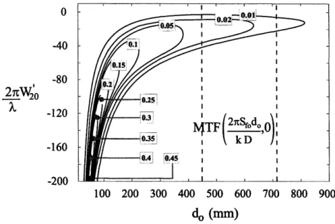
2-9 Behavior of the MTFe with respect to partial defocus (W20) and depth of field (do). The region between the dashed lines represents the depth of field of interest. The goal is to have maximum MTFe(uma(do), 0) = MTFe 2kD f,0 in this region. To do so we find the W20 for which MTFa2 (2DSfd,

O)

of this region of interest [see Eq. (2.22)]. This is justified by assuming that MTFa2 has a parabolic behavior with respect to W20. In this figure we have used ka = 10, kD2/8 = 104mm and 21rSfo/(kD) = 10-3mm- 1. . . .. . 46

2-10 MTFe(u, 0) of the system with and without pupil function engineering (Task-based imaging problem; optical system specifications are from Tables 2.3 and 2.4). The region between dashed lines represents the range of spatial frequencies of interest for that particular depth of field. Note how this range of spatial frequencies of interest gets smaller as the object gets closer to imaging system. (a) Traditional imaging system (far field, -- =a = -5), (b) Traditional imaging system (in focus, - = 0), (c) Traditional imaging system (near field, -- = +7), (d) Optimized imaging system (far field, !-W= = -4), (e) Optimized imaging system (in focus, E- = 0), (f) Optimized

2-11 The MTFe as a function of partial defocus and depth of field for the optimum sys-tem (task-based imaging problem; optical syssys-tem specifications are from Tables 2.3 and 2.4). The region between the dashed lines represents the depth of field of in-terest. The horizontal solid line represents the optimum value of W20. As it can be seen the goal of maximizing the MTF is achieved. Note how MTFe (27rSodo,l

MTFe (27f do2 ,o0 as it is expected from Eq. (2.22). . ... 52

2-12 Defocus of the (a) traditional imaging system and (b) imaging system with optimized pupil function engineering (Task-based imaging problem; optical system specifications are from Tables 2.3 and 2.4). Note how in the optimized imaging system the best focus is moved far from the imaging system to balance the modulation at the highest spatial frequency of interest over the entire depth of field. . ... 52

2-13 The minimum value of MTFe in the range of spatial frequencies of interest [namely MTFe(umax(do), O) = MTF(e (kD,0 O ] v.s. depth of field. The solid line rep-resents the optimized task-based imaging system and the dashed line reprep-resents the optimized uniform quality imaging system. This figure shows how the optimized uni-form quality imaging system is not efficient for task specific imaging. Note how the sub-optimization of Eq. (2.22) has increased MTFe (2 •Sfd , 0) over the depth of field of interest as shown by the solid-line graph. Optical system specifications are

from Tables 2.2 and 2.4. ... 53

2-14 Optimum cubic phase coefficient (a*) for task-based imaging. Using the range of interest for object (dol and do2), one can find the a* from this figure [Eq. (2.30)]. In this figure we have used A = 0.55 x 10-3mm, D = 8mm and Sfo = 14 line-pair . . 54

2-15 Optimum image-plane and exit pupil distance (d!) for task-based imaging. Using the range of interest for object (do₁ and do2), one can find the d' from this figure (Eq. (2.30)). In this figure we have used A = 0.55 x 10-3mm, D = 8mm, f = 50mm and

2-16 Graphical representation of the optimum cubic coefficient (uniform quality imaging problem). This figure is plotted using the optical system specifications provided Table 2.1. It shows how numerical optimization is in accordance with our analytical opti-mization. The optimum a from the figure is 4.65A whereas analytical optimization has shown a* = 4.60A. This difference is the result of the approximations performed

in Appendices B, C and D. ... ... 57

3-1 Schematic view of the optical system under consideration. . ... 62 3-2 Contour plot of the modulus of PSF, Ihj, in the presence of aberrations and defocus

(normalized to 100). ... . 71

3-3 Variation of the partial number of terms necessary with /3L,M for e = 0.001 and R* = 20. 76 3-4 Radial variation of the modulus of PSF with and without Distortion (normalized to

27r). . . . .. . . . .. . .. 77 3-5 Time required for evaluating PSF at 400 different points v.s. defocus (E = 0.1%). . 78 3-6 Time required for evaluating PSF v.s. resolution (e = 10%) ... . 79

4-1 Schematic view of the imaging system under consideration. O is the center of aperture, 00 is the center of the object plane and 01 is the center of the image plane. .,obj is the power leaving the object plane and .Ji is the power arriving at the image plane. Finally, D is the width of the aperture ... 84 4-2 Plot of spectral SNR as a function of defocus. . ... ... 93

B-1 Comparison of the imaginary error function and its approximation. . ... 108

C-1 Plot of exact (MTFe) and approximated MTF(u, 0) (MTFa2). Note how the exact

MTF has many oscillations whereas the approximated MTF does not. Also note that as a/A gets bigger, the accuracy of approximation gets better. (a) = 5,

W

List of Tables

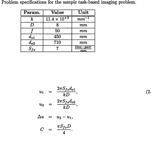
2.1 Problem specifications for the sample uniform image quality imaging problem ... 39 2.2 Optimized designed parameters for uniform image quality imaging problem ... 39 2.3 Problem specifications for the sample task-based imaging problem. . ... 49 2.4 Optimized designed parameters for the sample task-based imaging problem ... 50

Chapter 1

Introduction and Overview

One of the most important and perhaps first applications of the field of optics is imaging. Imaging systems have developed and got more and more complicated throughout the history. Each of these added complications has enhanced the performance of imaging systems in some way. These range from inventing new devices for recording the image to increasing the resolution of imaging systems to image ultra-small structures like atomic-level roughness of surfaces. In this thesis we focus on

one of such added complications: pupil function engineering.

1.1

Pupil Function Engineering

Pupil function engineering involves modification of the wavefront so that the imaging system meets a particular purpose. This modification often happens in the pupil plane, hence the name pupil function engineering. The pupil function can be considered as a complex function which is to be multiplied by the original wavefront at the pupil plane. This function has maximum amplitude of unity; in this thesis we only consider pupil functions which preserve the light collected by the imaging system; i.e. pupil functions that have amplitude of exactly equal to unity. This ensures that there is no absorption in the pupil plane.

Based on the above discussion, pupil function engineering in our context, consists of designing the phase function only. Note that pupil function is a function of pupil plane coordinates. So,

strictly speaking, one can think of our final designed pupil function as a physical object. This object (compare with contact lens that you wear everyday) modifies the phase of the incoming light and preserves the amplitude. It is clear that choices for pupil function is endless and that is precisely what makes the problem of pupil function engineering interesting. It should be added that pupil function engineering is often accompanied with a proper post-processing algorithm to get the final image. Although we do not cover the details of designing post-processing algorithms we do take into consideration the fact that post-processing algorithms exist. In fact, the final designed pupil function has to satisfy specific requirements to allow the use of post processing algorithms.

The ability to accurately and efficiently design an imaging system for a specific purpose is of increasing importance in the coming decades. Applications of imaging systems that have used pupil function engineering for this goal range from simple photography to advanced lithography machines. To mention some of the current application fields for pupil function engineering, we can name adaptive optics, phase retrieval, aberration correction, photography, general microscopy, optical lithography, integral imaging and computational tomography among others.

In this thesis, we study pupil function engineering, its tools, applications and limits from an analytic point of view. In Section 1.2 we motivate our approach by reviewing some the current problems in pupil function engineering and some of the potential benefits of our approach. In Section 1.3 we present the recent results in the literature related to this thesis and re-introduce our work in this context. Finally, in Section 1.4 we briefly mention our contributions in this thesis.

1.2

Motivation

The process of pupil function engineering, like any other design method has two main phases: (i) stating the imaging system requirements in the proper language, and (ii) finding the design parameters so that the imaging system meets those requirements. The challenge, however, seats in the transition from first phase to the second phase.

1.2.1

Computation Time Versus Accuracy

In imaging system design, there are a few different ways to mathematically state the imaging system requirements. Usually this is done by translating the system requirements to the language of either impulse response or frequency response of imaging systems. Two of the most important functions that are used for the analysis of imaging systems are the modulation transfer function (MTF) as a measure of frequency response and the point spread function (PSF) as a measure of the impulse response.

The process of transition from the MTF or the PSF to the final designed pupil function involves many instances of calculating PSF and/or MTF. In particular, depending on the number of possible degrees of freedom in final imaging system, the number of MTF and/or PSF calculation grows exponentially. As it is discussed in Chapters 2 and 3, based on a given pupil function, the calculation of MTF or PSF, each involves solving a double integral. This hints the process of pupil function engineering is very computationally expensive.

As it was mentioned in the previous Section, in pupil function engineering we are trying to design a phase value as a function of pupil coordinate and thus the complexity of final designed imaging system can be arbitrarily large. This increases the potential computational burden of the pupil function engineering even further.

This computational expense motivates us to look for a better way to relate the MTF and the PSF to the pupil function. In particular we are interested to find a relationship that allows us to move from pupil function to MTF and PSF fast and accurately. We view this as a major tool in pupil function engineering. In this thesis we have developed an approximate analytical relation between the MTF and the pupil function and the PSF and the pupil function.

1.2.2

Analytical Optimizations

In each iteration of pupil function engineering, the MTF or the PSF are calculated based on a given pupil function. This pupil function is, in turn, a result of a set of chosen design parameters. During the process of pupil function engineering the above iteration is repeated for many different design

parameters and in the end, a set of designed parameters is chosen as the optimal set. This set of design parameters is optimal in the sense that the MTF or the PSF resulted from the corresponding pupil function matches the stated MTF or PSF requirements the best.

An instant question that can be raises is what do we know about optimality of the final pupil function. For instance we would like to know if our result is the global optimum or not. In fact, in finite iterations of the above algorithm we cannot guarantee anything about global optimality.

An alternative to the above approach is to use analytic optimization algorithms; however to do so we need to have a closed form expression relating the MTF and the PSF to the pupil function. It is well-known that such a relation does not exist except in the integral form and thus this motivates us to develop analytic approximate expressions relating the MTF and the PSF to the pupil function.

1.2.3

Physical Understanding

Due to the high complexity of pupil function engineering, usually the optimization process and result

carry no or little intuition about the physics of the problem. In particular, there are many classes of problems that pupil function engineering is known to be well-suited for; nevertheless the physical limits of pupil function engineering for most of these problems has not been studied and is not known.

For instance, consider the problem of extension of depth of field. It is known that pupil function engineering can extend the depth of field. There has been many instances of successful imaging system designs that have used this. Yet, there are some unanswered fundamental questions in this regard. One of the fundamental questions in this regard is: to what extent one can extend the depth of field of an imaging system using design and optimization of the pupil function? Questions of this nature, motivate us to study the pupil function engineering analytically. Also, during the optimization process itself, having an analytic expression for the problem can help the designer a lot as to what are the important parameters, what are the sensitive parameters, etc.

1.3

Background

In this section we perform a quick review of results related to pupil function engineering. In par-ticular, we present results related to both numerical and analytical approaches in pupil function engineering. Finally, we consider the depth of filed and results related to extension of depth of field.

1.3.1

Numerical Results

Traditionally calculation of MTF and PSF using a specific pupil function has been done numerically. One way of doing this is to directly calculate the finite Riemann sum as an approximation to the final integral. It is a common practice to use fast Fourier transform (FFT) rather than direct integration to enhance the speed of calculation. However, the FFT method also fails to perform well as the resolution of interest or the accuracy of interest increases. In what follows we review the performance of FFT for calculation of PSF using a given pupil function. Note that MTF and PSF are related using Fourier optics and thus the same discussion applies to MTF as well.

Here we quickly review the trade off between accuracy and computational expense in the FFT method [1, 2]. In imaging systems we are usually interested in two-dimensional FFTs. The number of calculations necessary for a two-dimensional FFT of an A' x ~ array is 2.Y'2 _{log 1Y2. Thus the}

time necessary is proportional to this expression too. In computational imaging systems we take the FFT of the pupil function to get PSF. Accuracy of FFT highly depends on the complexity of the pupil function. This is because as this complexity increases the fixed number of sample points fail to capture the complexity of pupil function well.

This has serious drawbacks in optimization algorithms. First, during each iteration the com-plexity of pupil function changes and thus to keep accuracy fixed we need to change the FFT size appropriatly. This makes the optimization algorithm more complicated.

Secondly, as it was shown above the number of sample point and thus the calculation burden grows very fast with the complexity of pupil function. In particular, this limits our design abilities to incorporate more complicate pupil functions in imaging systems.

1.3.2

Analytical Results

There has been many efforts to analytically approximate important functions in imaging systems. For the same reason as last Section, we only consider PSF and methods to analytically approximate this function. The original Nijboer-Zernike method that can be applied to very simple pupil function has very limited application. [3] Recently, extensions of the original Nijboer-Zernike method have been developed in order to make it applicable to more complicated pupil functions. These expansions lead to a representation of the PSF whose complexity increases at least linearly with defocus [4, 5, 6, 7]. This means given a class of pupil functions, as the value of some of the parameters increases, the complexity of the calculation increases too.

1.3.3

Depth of Field

A common problem encountered in the design of imaging systems consists of finding the right balance between the light gathering ability and the depth of field (DOF) of the system. Having high signal-to-noise ratio (SNR) at the detector of an imaging system over a large range of depths of field has

been the utmost goal in many imaging system designs [8, 9, 10].

Traditionally, most of the attention in the literature has been focused on increasing the depth of field for special problems of interest. This typically includes cases of successfully designed imaging systems that work in an extended depth of field. Usually in these systems SNR is shown to be within acceptable limits depending on the particular goal. There are however cases in which a subclass of design problems (for instance, cubic-phase pupil function) are studied analytically where the limits of extension of depth of field in terms of generic acceptable SNR is discussed more rigorously [11, 12, 9, 13, 14].

Traditionally (as we have all experienced with our professional cameras) one can extend the depth of field by controlling the aperture stop size. Albeit very simple, this method has serious drawbacks such as significantly reducing the optical power available and the highest spatial frequency [15]. This limits the practical use of this method to very short ranges of depth of field [16]. Pupil function engineering combines aspheric optical elements and digital signal processing to extend the depth

of field of imaging systems. [17, 18, 19, 20]. Although numerous important industrial problems are solved using pupil function engineering, there is no concrete statement about the extent pupil function engineering can improve SNR over the depth of field of interest.

1.4 Contribution

In this thesis, we study pupil function engineering, its tools, applications and limits from an analytic point of view. In particular, we derive approximate analytic expressions for the MTF and the PSF. Using our expressions one can save a lot of computational power at a practically negligible accuracy expense. We solve some optimization problems using our expressions. We also answer the fundamental question regarding the extension of depth of field in imaging system.

In Chapter 2, we derive an approximate analytical expression for the MTF of an imaging system possessing a shifted cubic phase pupil function. We derive the error bounds of our approximation and establish its high accuracy (see Theorem 2.2.1). Using the approximate representation of the MTF we solve the problem of extension of depth of field analytically for two cases of interest:

uniform quality imaging and task-based imaging. We also show how the analytical solutions given

in this Chapter can be used as a convenient design tool as opposed to previous lengthy numerical optimizations.

In Chapter 3, we introduce a new method for analyzing the diffraction integral for evaluating the PSF. Our approach is applicable when we are considering a finite, arbitrary number of aberrations and arbitrarily large defocus simultaneously. We present an upper bound for the complexity and the convergence rate of this method (see Theorem 3.5.1). We also compare the cost and accuracy of this method to traditional ones and show the efficiency of our method through these comparisons. This has applications in several fields that use pupil function engineering such as biological microscopy, lithography and multi-domain optimization in optical systems.

In Chapter 4, we discuss the limit of depth of field extension for an imaging system using pupil function engineering. In particular we consider a general imaging system in the sense that it has arbitrary pupil-function phase and we present the trade-off between the depth of field of the system

and the spectral SNR over an extended depth of field. Using this, we rigorously derive the expression for the tightest upper bound for the minimum spectral SNR, i.e. the limit of spectral SNR improve-ment (see Theorem 4.4.1). We also draw the relation between our result and the conservation of brightness theorem and establish that our result is the spectral version of the brightness conservation theorem. Finally, we conclude in Chapter 5.

Chapter 2

Modulation Transfer Function

In this Chapter we derive an approximate analytical expression for the modulation transfer function (MTF) of an imaging system possessing a shifted cubic phase pupil function. This expression is based on an approximation using Arctan function. Using the approximate representation of the MTF we solve the problem of extension of depth of field analytically for two cases of interest:

uniform quality imaging and task-based imaging. We derive the optimal result in each case as a

function of the problem specification. We also compare the two different imaging cases and discuss the advantages of using our different optimization approach for each case. We also show how the analytical solutions given in this Chapter can be used as a convenient design tool as opposed to previous lengthy numerical optimizations.

2.1 Introduction

Pupil function engineering is a computational imaging technique used to greatly increase imaging performance while reducing the size, weight, and cost of imaging systems [18]. It consists of the combined use of optical elements with digital signal processing in order to better perform a required imaging task. For example, pupil function engineering can be used to extend the depth of field of an imaging system [17, 21]. In traditional (without pupil function engineering) imaging systems, such an extension of the depth of field is usually obtained by reducing the aperture stop, consequently

reducing the resolution and light gathering capacity of the imaging system. Because pupil func-tion engineering elements typically are non-absorbing phase elements, they allow the exposure and illumination to be maintained while producing the depth depth of field of a slower system [18, 20].

A challenging process in designing systems with extended depth of field is choosing the right phase element. The design goal is to make the point spread function (PSF) of the optical system defocus-invariant; i.e. to make the PSF of the optical system shape-invariant as the object moves along the desired depth of field. Having a defocus-invariant PSF facilitates the image reconstruction using a simple deconvolution filter. Simultaneously, one tries to keep the MTF as high as possible as the object moves along the desired depth of field. This is done, in order to transfer the most information possible from the object to the optical sensor. Here, by the most information possible we refer to the space bandwidth product of the imaging system or in other words the maximum number of resolvable spots [22, 23, 24].

One of the phase elements that is most often used in practice is described by a cubic phase,

#(i,

9),

4D(,

_{=a [(I + 6)}

_{+ (ý + j)3].}

where a is the cubic phase coefficient, 6 is the cubic phase shift and (^, ý) are the normalized

Cartesian coordinates at the pupil plane.

This phase surface has some interesting properties; among which is the fact that the PSF of the optical system which is equipped with this phase element is defocus-invariant. This property makes this phase element an excellent choice for the problem of extension of the depth of field. Having chosen this type of phase element the design usually consists of numerically maximizing the MTF of the optical system. The optimization parameters are phase element parameters (e.g. a) and optical system parameters (e.g. distance between the image plane and the exit pupil) [24].

This process of numerical design and optimization is lengthy and time consuming, for one needs to numerically evaluate the MTF for every variation of design parameter values, and a large number

of parameter values have to be visited. Furthermore this process needs to be redone for every and each specific problem. On top of all this, there is no theoretical guaranty that one is actually reaching the global optimum design within a limited time of numerical optimization [25, 26].

In this Chapter we offer an alternative to numerical optimization by modeling and solving the design problem analytically. This is mainly a result of our developed approximation to MTF. We derive the expression for a generalized MTF with cubic phase element in pupil plane. In this model we assume a diffraction-limited lens, an incoherent illumination and a cubic-phase element. We perform an accuracy analysis and show that the developed approximation has a very good accuracy (97% on average) in the regions of interest in imaging design.

This model provides us with the MTF as a function of defocus. This generalized MTF is then used to optimize the imaging system. We analytically solve the cubic phase element design and optimization problem for two general imaging problems. These two problems are: (i) to extend the depth of field for uniform image quality imaging systems (e.g. normal photography, cellphone cameras, etc. ) and (ii) to extend the depth of field for task-based imaging systems (e.g. bar code reader, iris recognition, etc.).

In the next Section we derive the analytic MTF representation, which will be used as a basis for our optimization in the rest of the Chapter. In Section 2.3 we solve the problem of extending the depth of field for the case of imaging with uniform image quality. We go over the optimality criteria and we solve the optimization problem analytically. We present an example and show how our results apply in solving a practical problem. In Section 2.4, we solve the problem of extending the depth of field for task-based imaging. In Section 2.5 we compare both results from Sections 2.3 and 2.4 a nd discuss their relative benefits. We also go over some of the general results that could be deduced from the optimal solution graphs and their applications to design problems.

2.2

Analytic MTF

In this Section we derive an analytic approximation for the MTF of an imaging system with a cubic phase element installed in its aperture. We assume an imaging system with circular aperture being

illuminated with incoherent light. Figure 2-1 shows a schematic view of our optical system. Using simple Fourier optics one can get the expression for MTF of such optical system. Note that the ultimate goal of this chapter is to maximize MTF. However there is a fundamental limit to that due to the conservation of ambiguity function. It has been observed that generally the most efficient way of managing this limit is to maximize MTF only on two orthogonal axis, thus keeping the used portion of this fixed area as small as possible [27, 28, 29]. Please see Appendix A or Chapter 4 for more detailed discussion. Due to the symmetry of problem, it suffices to analyze MTF in any of these two orthogonal directions. Thus, we can continue with the revised version of the MTF equation as below

MTFe(u,O)= 1 1•• eki(4W2ou) ~+(6au) i2] did d , (2.1)

where MTFe is the exact value of MTF, ^ and ý are normalized Cartesian coordinates of the pupil,

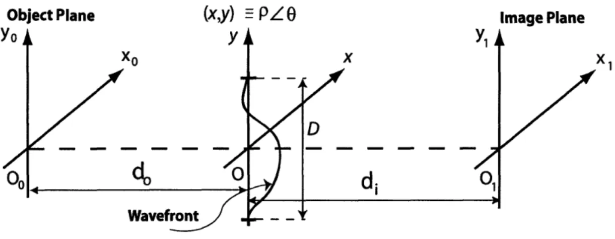
u and v are normalized spatial frequencies in : and ý directions respectively, W20 = (D2/8) (1/di +l/do - 1/f) is the defocus coefficient and a is the cubic-phase coefficient; k = 2rn/A, f, di, do

and D are the wave number, imaging system focal length, distance from the image plane to the exit pupil, distance from the object plane to the entrance pupil and aperture diameter respectively. The last three parameter definitions are illustrated in Fig. 2-1. Note that W20 has the dimension of length. Finally, xm and y, are defined as

Xm =

V/-

Ym = -- U2 .

The details of derivation of Eq. (2.2) is given in Appendix A. At this point we have two integrals which cannot be analytically evaluated in a closed form. In particular, for any set of imaging system parameters calculating the value of MTF requires numerical calculation of a double integral. This is

Object Plane

(x,y) H PZ o

di

Image Plane

Figure 2-1: Schematic view of optical system under consideration.

often very expensive during a design process which requires many instances of MTF calculation. To overcome both of these problems (lack of closed form solution and computational cost), we introduce an approximation for MTF. Our results are based on the following novel approximation:

x _exp(it2_{)dt - Arctan}

_(v'

o0V2

(2.3)

Based on Eq. (2.3) we have deriven two different approximations for MTF. The first approx-imation, MTFal is suitable for numerical calculation and the second approxapprox-imation, MTFa2_{, is} suitable for analytic manipulations. The detailed derivation of these two approximations can be found in Appendices B and C, respectively. In the subsequent Sections we use MTFa2 _{as our MTF} approximation. The expression for MTFal is too lengthy and thus is skipped. The expression for

MTFa2is shown below

MTFa2(u,) 2 -Arcsin(u) + ru x (2.4)

Arctan

2r

[W2o + 3a(1

-

u)]

-Arctan

_V7r

ku

[W20

+ 3(-+

Equation (2.4) above is the approximate analytic expression for the MTF. Note that u in this equation is the normalized spatial frequency (when u = 1, the system is at the diffraction limit). This expression for the MTF makes the analytic solution of an optical design problems that involves MTF mathematically tractable.

Before using any of these two approximations, we need to investigate their accuracy. The accuracy of MTFal and MTFa2 are studied in Appendices B and C, respectively. Here we present some of the results in this regard.

Theorem 2.2.1. Let e be the approximation accuracy and C be the sub-space of interest in design parameters space, such that

IMTFe(u, O) - MTFal(u, )I 20E(&, 20, u),

and

C {0.2 < u < 1} x {2 < & < 10} x 0 < W20 < 8}.

Then, we have

max

• e(,

20,U} < 0.1,

if

I

E(&,

'20,

u)

d&

dlV20o

du

0.03,

0.1

E ( ,4,

u)0.09

I

X

10

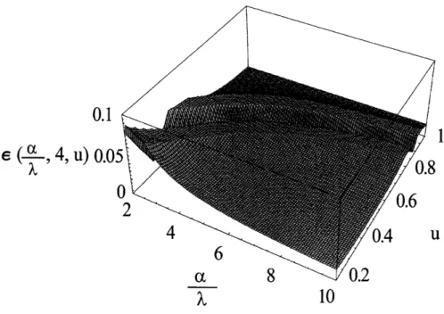
Figure 2-2: Plot of e (&, 4, u) as a function of & and u (Note that all variables are dimensionless).

and

IMTFa

_-

_{MTFalI <}

_0.1.

In Theorem 2.2.1, & = a/A and W₂₀ = W20/A are normalized cubic phase coefficient and nor-malized defocus coefficient, respectively. The function E(&, W20, u) is a bound of our approximation error. The immediate interpretation of these results would be the high accuracy of MTF"

_a.

shown in Theorem 2.2.1 the difference between MTFa2

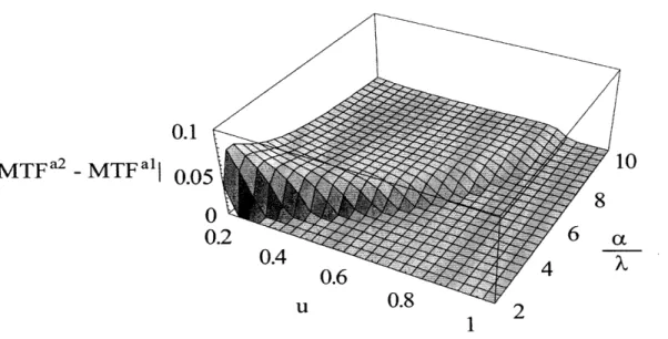
and MTFal is bounded. Figure 2-3 shows the plot of jMTFa2 - MTFal as & and u varies while W20 = 4.

It should be noted that most of the results in Theorem 2.2.1 are representing the worst-case scenario. The real power of these approximation is in their average accuracy [for instance see Eq. (B.26)]. This is because during optimization process the average behavior of the approximation over the parameters of interest matters the most. It should be also noted that the only advantage of

0.1

IMTFa

_-

_{MTFall 0.05}

(

(

0

Figure 2-3: Plot of MTFa2 - MTFal as a function of & and u when 720 = 4 (Note that all variables are dimensionless).

optimization, then MTFal is the approximation expression to be chosen. This is because it has a good accuracy and a closed form expression and hence much easier to compute compared to MTFe which involves the calculation of a double integral.

Finally it is worth mentioning that although these MTF expressions only consider defocus and cubic phase shift, one can employ the same approach to incorporate other aberrations into the approximate MTF expressions. The key is to capture the mean behavior of the integrand and then do the integral. This way, one first keeps the accuracy high and second makes the job of evaluating the integral simple. To expand these MTF expressions to other aberrations is one of the possible future work directions.

In the next two Sections we show how by using this expression we can solve two classes of design problems that illustrate well the use of the cubic phase pupil function to extend the depth of field of an imaging system. In the first problem we discuss the uniform image quality imaging and in the second problem we discuss the task-based imaging.

2.3

Optimization for Uniform Image Quality

2.3.1

Statement of the Problem

A well-known challenge in imaging systems is how to maintain a uniform image quality as the object

moves along the depth of field of interest [21, 18]. The term image quality is clearly very broad and, in general, the image quality not only depends on the imaging system but also on the object spectrum. In this Chapter, by image quality of an imaging system, we precisely mean two factors: (i) the range of spatial frequencies that can be transfered from the object to the image plane and (ii) the transfer function of the imaging system for this range of spatial frequencies. Thus a uniform

image quality imaging system has (i) a fixed range of transferable spatial frequencies as the object

moves through the desired range of depth of field and (ii) a uniform transfer function for that range of spatial frequencies as the object moves through the desired range of depth of field.

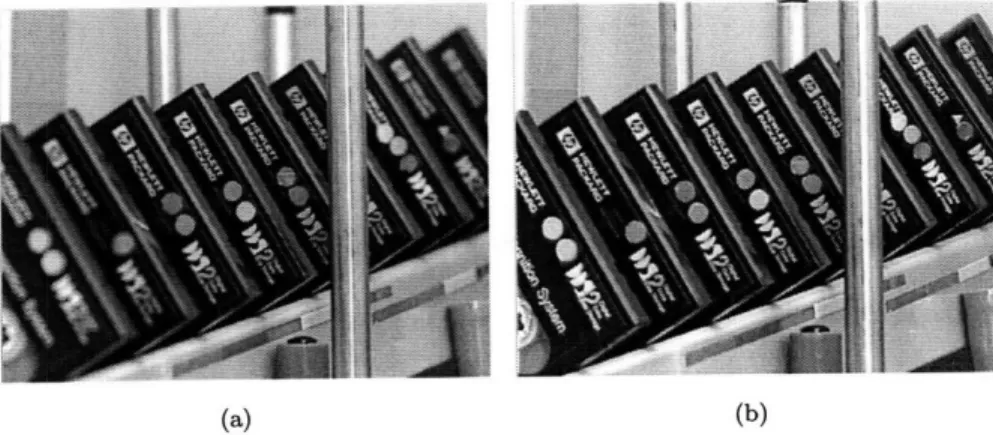
The design goal in this Section is to increase this uniform image quality. We assume that the range of the spatial frequencies of interest is given as a design specification and we try to maximize the transfer function of the imaging system for that range of spatial frequencies as the object moves through the desired range of depth of field. This is what we mostly encounter in typical photography. In this type of imaging systems, one is interested in getting a high quality image for some desired range of depths of field. Another example in typical photography is when we focus on a particular object and we would like to have a uniform quality over all parts of the image; i.e. not only the part we have focused on, but also in all other parts of the picture. This means we want to have a uniform image quality as we are moving through some depths of field of interest [30]. This is further clarified in Fig. 2-4. This figure shows two pictures taken from a non-planar object. The object is a stack of printer cartridges. They are positioned so that the leftmost is closest to the imaging system and the rightmost is furthest from the imaging system. Part (a) is the picture taken by a traditional imaging system. As it can be seen the image quality is not uniform in this picture. Part (b) is the picture taken by an imaging system which uses pupil function engineering. As it can be seen, this picture has a uniform quality over the range of depth of field of interest. In other words,

(a) (b)

Figure 2-4: Photos of a non-planer object with (a) traditional imaging system and (b) imaging system with pupil function engineering. Part (a) does not have a uniform image quality. Quality is good at best focus in the center of the photo and image gets blurry out of focus. Part (b) has a uniform image quality; i.e. the image quality is the same both in and out of focus. Here by uniform image quality we mean the uniform transfer function of the imaging system at the spatial frequencies of interest over the depth of field.

in part (b) the transfer function for the range of spatial frequencies of interest is uniform over the depth of field of interest, and thus the image quality is preserved in the depth of field of interest.

In this context the design goal can be stated as maximizing the entire MTF (which is a measure of the transfer function of the imaging system as a function of spatial frequencies) over the imaging volume. The optimization problem will be defined in a way to reach this goal.

Considering the preceding imaging design problem, the typical problem specifications are: range of object distances (range of do), focal length (f), aperture diameter (D), and maximum spatial frequency of interest for the image (Sfi). Using these fixed problem specifications and through the optimization process we find the design parameters: cubic phase coefficient (a) and image-plane to exit-pupil distance (di). Our goal is to find the design parameters that satisfy the following optimality criterion

max min { MTFa2_{(u, 0)} (2.5)}

a,di do,u

di Ei R

do E [dox, do2]

u

E [0,

Umax]

Equation (2.5) along with Eq. (2.4) are used as the basis of the optimization in Section 2.3.2. The analytic expression for design parameters (a and di) are found as a solution of the optimization problem.

2.3.2

Optimization

In this Section we solve the optimization problem stated in Eq. (2.5). We begin with a discussion about the highest normalized spatial frequency in the image plane, umax. Since our aim is to have

uniform image quality, umax is constant over the range of optimization parameters. Its value is

defined using the highest spatial frequency of interest for the image (Sfi) as below

Umax =

Si

2fo

where fo is the diffraction limited spatial frequency of the coherent imaging system. Thus we have

Umax rdSf (2.7)

kD

Now, considering Eq. (2.4) and using the fact that MTFa2_{(u, 0) is monotonically decreasing}

equivalent to setting u = Umax. Hence, we can rewrite Eq. (2.5) as

max min ( •MTFa2 i . (2.8)

av,di d\

kD

di E R

do E [dol,do2]

The next step is the minimization of the MTFa2 over do and the maximization of the MTFa2 over di. In fact these two steps are coupled, for they both have a direct effect on W20, and thus on the system's defocus, as it is explicitly shown in Eq. (A.6). In this step, we use the fact that increasing the absolute defocus (W20) reduces MTFa2 and vice versa (see Appendix E for details). Since increasing the absolute defocus reduces MTFa2 and vice versa, one can define a sub-optimization problem for these two parameters as shown below

min

m{ax {,W

} }.

di c R

d

E [do,,

Recall that W20 is given by Eq. (A.6). Using elementary calculus, one can solve the problem above to find

2fdoldo2

d _2dold 2fdodo2 (2.10)

o2 - f(do + do 2)'

Thus we can rewrite Eq. (2.8) as

max {MTFa2 (Umax, 0)}, (2.11)

where umax is defined through Eqs. (2.7) and (2.10) and W20 is defined through Eqs. (A.6) and (2.10). Note that neither Umax nor W20 is a function of a and thus one can easily deal with this optimization problem without worrying about the complicated formulas for umax and W2 0 (As we

will see, this is not the case in Section 2.4).

To solve Eq. (2.11) we find the maximum value of the MTFa2 by setting its first derivative

equal to zero

BMTFa2(o)_{MFa = 0.}

(2.12)

aa

Note that this approach is only feasible because we are using an approximation to the exact MTF. In fact, the exact MTF is a highly oscillating function, and such an approach for finding the optimal cubic phase coefficient (a*) is of little use. Strictly speaking, in case of the exact MTF, Eq. (2.12) does not have a unique solution in the regions of interest in imaging design. However, our approximation (MTFa2) which represents the average value of this oscillating function (MTFe ) results in a unique optimal value for the cubic phase coefficient (a*) which could be found through Eq. (2.12) (See Appendix E for more details about the properties of our approximation). This fact allows solving Eq. (2.12) for the optimal cubic phase coefficient (a*). An approximate solution to Eq. (2.12) is found in Appendix D. The result is as follows

a* 1 + 8umax (1 -Umax) + 1 + 16umax (1 - Umax)

SX

V

(2.13)

,

_(2.13)

where umax is defined through Eqs. (2.7) and (2.10) and W20 is defined through Eqs. (A.6) and (2.10). In Section 2.3.3 we will discuss the optimization results obtained in this Section.

2.3.3

Results

In this Section we discuss the results of the optimization which was done in the last Section. We use a sample problem to clarify the benefit of using this method. We also present the graphs of the general results along with a method of how to use these graphs in a practical optical design problem. We begin with presenting the final results of optimization in Eqs. (2.14). As it could be seen through these equations, all the design parameters are expressed in terms of the problem

specifica-tions; i.e. f, D, k, do1, do2 and Sfi.

a*

1

a

=

A(2.14)

A

(2.14)

S = 2

fdold

where Umax and W20 are

Uma = 21rdSf (2.15)

kD W20 = 2 (-di

8

di

f/

In order to illustrate the results of the optimization, we use a sample imaging design problem, whose specifications are shown in Table 2.1. The wave number, k = 2rxn/A, is chosen to be the

average value for visible light propagating in air. The aperture diameter, D, and the focal length, f are chosen so that we have a practically feasible f# at a reasonable cost. The required depth of field, i.e. dol and do2, which should be chosen according to the goal for the range of functioning of imaging

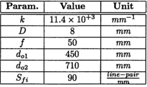
Table 2.1: Problem specifications for the sample uniform image quality imaging problem.

Param. Value Unit

k 11.4 x 10+ 3 _mm -D 8 mm f 50 mm do1 450 mm do2 710 mm

Sf

90

Table 2.2: Optimized designed parameters for uniform image quality imaging problem. Param. Value Unit

4.60

-dr 55 mm Umax 0.34

-= 6

-system, is chosen to be in accordance with its corresponding value in the sample task-based problem so that one could compare results obtained for each method. The maximum spatial frequency of interest in the image plane, Sfi, is chosen with the same goal in mind.

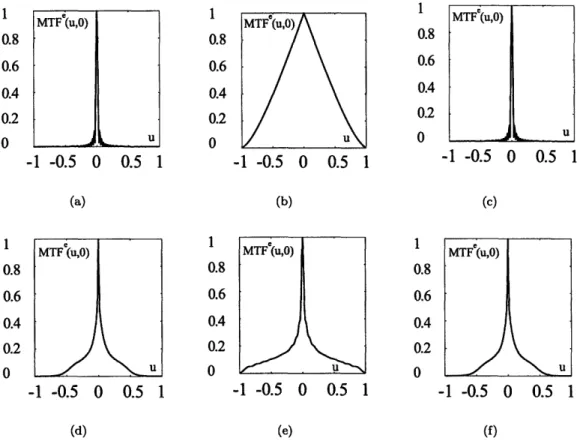
Using the problem specification values presented in Table 2.1, one can get the optimized design variables using Eqs. (2.14) and (2.15). These values are shown in Table 2.2. To compare the performance of the optimized imaging system with that of the traditional system (without pupil function engineering: di = 54.7mm and a = 0), we have shown the plot of the MTFe

at three different depths of field for these two systems in Fig. 2-5. Using this figure, one can see how the

MTFe has been distributed over the entire field rather than just at the in-focus plane. One can also see that the worst-case MTF (minimum MTFe in the union of the range of interest of all variables) is 0.10. Also, the graph of defocus, W20, versus depth of field is shown in Fig. 2-6. This graph shows that we have actually minimized the maximum absolute value of defocus along the desired depth of field; i.e. we have reduced W₂₀ from 7A to 6A. Note that, in the optimized system, the best focus has moved from the middle of depth of field toward the lens. In particular do for best focus is reduced from 0.58 m to 0.55 m. This is due to nonlinear relationship between W20 and d,.

specifi-MTFe(u,O)

u

-1

-0.5

0

0.5

1

(a)

-1

-0.5

0

0.5

1

(d)

-1

-0.5

0

0.5

1

(b)

-1

-0.5

0

0.5

1

(e)

f

-1

-0.5

0

0.5

1

(c)

-1

-0.5

0

0.5

1

Figure 2-5: MTFe(u, 0) of the system with and without pupil function engineering (Uniform image quality imaging problem; optical system specifications are from Tables 2.1 and 2.2). Note how image quality (the transfer function of the imaging system at the spatial frequencies of interest) is uniform over the depth of field. (a) Traditional system (far field, -- = -5). (b) Traditional system (in focus, -W- = 0). (c) Traditional system (near field, -- = +7). (d) Optimized system (far field,

W2& = -6). (e) Optimized system (in focus, -W- = 0). (f) Optimized system (near field, - = +6).

20 o

4

do(mm)

m)

Figure 2-6: Defocus of the (a) traditional imaging system and (b) Optimized imaging system in uniform quality imaging problem (Optical system specifications are from Tables 2.1 and 2.2). Note that in the optimized imaging system the best focus has been moved toward the lens to reduce the maximum absolute defocus from 7A to 5.5A.

k--

U

--15 C* 10

x

5

0

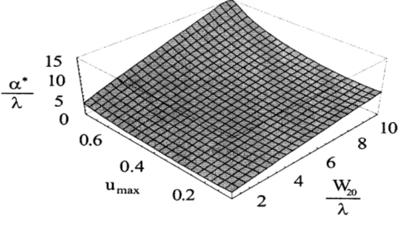
10

Figure 2-7: Optimum cubic phase coefficient (a*) for the uniform image quality problem. Using given problem specifications one can find the corresponding umax and W20 (Eq. (2.15)), and then a* can be directly read from this figure [Eq. (2.14)].

cations and evaluate W20 and Umax through Eqs. (2.15) and then use these values for evaluating d* and a* through Eqs. (2.14). Figure 2-7 shows the optimal value of the cubic phase coefficient versus defocus and image quality (maximum spatial frequency of interest in the image plane).

2.4

_{Optimization for Task-based Imaging}

2.4.1

Statement of the Problem

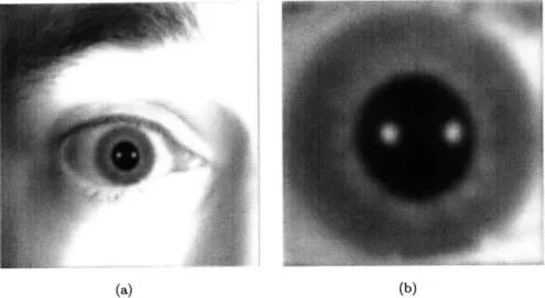
Task-based imaging systems have played an important role in the development of industrial appli-cations and in the improvement of living standards in recent years. These roles range from simple bar code reading in a supermarket to complicated identification systems in high-security facilities (for instance, biometric iris recognition [20]). A critical challenge in this field is to have a sufficiently good image in a certain depth of field, in the sense that this image must be usable for the specific task. Particularly, for task-based imaging it is immaterial whether the picture looks good or not. Rather, the amount of usable information that is transfered from the target object to our detective device is of utmost importance. In general, this means we need more resolution when the image is smaller and less when the image is bigger. This is clarified further in Fig. 2-8, which shows two photos are taken by an iris recognition system. As it can be expected, the system is only concerned

(a) (b)

Figure 2-8: Iris recognition images as an example of task-based imaging. (a) Far field image (do = 800mm). (b) Near field image (do = 200mm). Although part (a) appears to be a higher quality

image, parts (a) and (b) both have equal usable information of iris.

about the amount of information that it captures from the iris. Thus, as the person gets closer to the device, the required resolution decreases so that the amount of information from the iris remains constant. Although part (a) may be considered a good picture and part (b) a poor one from the photography point of view, they are both equally good from a task-based point of view.

In the design process of a task-based imaging system, it is crucial to take the above point into account. It is often the case that we want to capture a constant amount of usable information from the object as the object is moving along a desired depth of field. This instantly calls for the use of pupil function engineering. However, in this case the optimal design criterion would be different

from the one we discussed in the last Section.

In an imaging problem like this, the classic problem specifications are depth of field of interest, i.e. the range along which the object can move (range of do), focal length (f), aperture diameter (D), and maximum spatial frequency of interest for the object, i.e. the maximum amount of detail from the object that we need to capture for our specific task (Sf,). Using these problem specifications and through the optimization process we find the design parameters, which are the cubic phase coefficient (a) and the image-plane to exit-pupil distance (di). Our goal is to find design parameters that satisfy the optimality criterion. This is expressed in Eq. (2.16):