Design and modeling of a high flux cooling device based on thin film evaporation from thin nanoporous membranes

DESIGN AND MODELING OF A HIGH FLUX COOLING

DEVICE BASED ON THIN FILM EVAPORATION FROM

THIN NANOPOROUS MEMBRANES

|M

MASSACHUSETTS INWTr

by OF TECHNOLOGY

Zhengmao Lu O

B.S., Tsinghua University (2012)

LIBRARIES

Partial Fulfillment of the Requirements for the Degree of Master of Science in Mechanical Engineering

at the Massachusetts Institute of Technology September 2014

C 2014 Massachusetts Institute of Technology

All rights reserved

Signature of Author:

Signature

redacted

Department of Mechanical Engineering August 27, 2014

Certified

by:

SignatUre

redacted

Evelyn N. Wang Associate Professor of Mechanical Engineering

Signature redacted

Accepted by:...

David E. Hardt Chairman, Department Committee on Graduate Theses

DESIGN AND MODELING OF A HIGH FLUX COOLING DEVICE

BASED ON THIN FILM EVAPORATION FROM THIN

NANOPOROUS MEMBRANES

by

Zhengmao Lu

Submitted to the Department of Mechanical Engineering on August 27t, 2014 in Partial Fulfillment of the Requirements for the Degree of Master of Science

Abstract

Heat dissipation is a limiting factor in the performance of integrated circuits, power electronics and laser diodes. State-of-the-art solutions typically use air-cooled heat sinks, which have limited performance owing to the use of air. One of the promising approaches to address these thermal management needs is liquid vapor phase-change.

In this thesis, we present a study into the design and modeling of a cooling device based on thin film evaporation from a nanoporous membrane supported on microchannels. The concept utilizes the capillary pressure generated by the small pores to drive the liquid flow and largely reduces the viscous loss due to the thinness of the membrane. The interfacial transport has been reinvestigated where we use the moment method to solve the Boltzmann Transport Equation. The pore-level transport has been modeled coupling liquid transport, vapor transport and the interfacial balance. The interfacial transport inside the pore also serves as a boundary condition for the device-level model. The heat transfer and pressure drop performance have been modeled and design guidelines are provided for the membrane-based cooling system. The optimized cooling device is able to dissipate 1 kW/cm2 _{heat flux with a temperature rise less than 30 K from the vapor side. Future}

work will focus on more fundamental understanding of the mass and energy accommodation at the liquid vapor interface.

Thesis Supervisor: Evelyn N. Wang

Acknowledgement

I would like to express my gratitude to my advisor, Professor Evelyn Wang, for her careful guidance over the past two years. This work could not have been possible without the help and support from her.

I would also like to thank all the students, postdocs and alumni in the Device Research Laboratory

for all the thoughtful discussions. I would like to especially thank Dr. Shankar Narayanan, Dr. Rong Xiao, and Kevin Bagnall for their insightful advice and I also gratefully acknowledge the

funding support from Defense Advanced Research Projects Agency (DARPA).

I am grateful that I have met David Bierman, Dan Preston, Kyle Wilke and Daniel Hanks, who make my life much easier and more exciting as an international student at MIT.

Finally, I would like say thank you to my girlfriend, Jie Zhou, and my family for their unwavering love and support.

Table of Contents

1. INTRODUCTION . ...

1.1 MOTIVATION...11

1.2 BACKGROUND...12

1.3 THESIS OBJECTIVES AND OUTLINE...14

2. _{MODEL FRAMEWORK ...---...---.---... 15}

2.1 PRESSURE DROP ...---... ₁₅

2.2 HEAT TRANSFER...16

3. _{INTERPHASE MASS TRANSFER... ... ... 17}

3.1 PROBLEM FORMULATION.... ... ... ... 17

3.2 _{PREVIOUS APPROACH ... 18}

3.3 CURRENT APPROACH ... ₁₈

3.4 SU M M A R Y ... ₂₁

4. PORE-LEVEL TRANSPORT...--.---...22

4.1 PROBLEM FORM ULATION ... ₂₃

4.2 MODEL DESCRIPTION...26

4.4 SU M M A R Y ... .. ... ... 34

5. DEVICE PERFORMANCE MODEL ... 35

5.2 PARAM ETRIC SW EEP ... 37

5.3 SUM M ARY...- -... -41

6. CONCLUSIONS AND ONGOING WORK ... 42

7. BIBLIOGRAPHY ...--.----.--- 44

APPENDIX...----.---.7

LIST OF FIGURES

FIGURE 1 HIGH POWER ELECTRONICS THAT CAN GENERATE INTENSIVE EXCESSIVE HEAT FLUXES: (A) RF POWER AMPLIFIER [5] (B) LASER

DIODE ARRAYS [6). ... 11

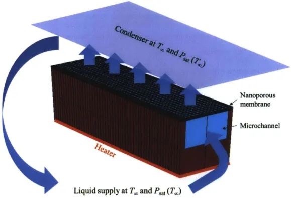
FIGURE 2 A THIN NANOPOROUS MEMBRANE-BASED COOLING DESIGN: LiQUID IS DRIVEN INTO THE NANOPORES VIA THE

MICROCHANNELS WITH THE HELP OF THE HIGH CAPILLARY PRESSURE GENERATED BY THE NANOPORES. HEAT CONDUCTS THROUGH

THE CHANNEL WALLS, SPREADS THROUGH THE MEMBRANE AND THEN ARRIVES AT THE LIQUID VAPOR INTERFACE WHERE

EVAPORATION TAKES PLACE. ... 13 FIGURE 3 ONE WORKING UNIT OF THE COOLING DEVICE: PERIODIC BOUNDARY CONDITIONS ARE APPLIED TO THE LATERAL WALLS, A

CONSTANT HEAT FLUX IS APPLIED TO THE BOTTOM OF THE DEVICE AND THE EVAPORATIVE FLUX NEEDS TO BE ADAPTER FROM THE

PORE-LEVEL TRANSPORT... 16

FIGURE 4 FORMULATION OF THE ONE-DIMENSIONAL STEADY STATE EVAPORATION FROM HALF-SPACE PROBLEM: THE VAPOR FLOW IS

FIRST OF VERY HIGH NON-EQUILIBRIUM AND THEN RELAX ITSELF TO REACH EULER EQUILIBRIUM ... 17 FIGURE 5 INTERFACIAL HEAT FLUX AS A FUNCTION OF THE TEMPERATURE RATIO BETWEEN THE EVAPORATING SURFACE AND THE FAR

FIELD VAPOR FOR THREE DIFFERENT FLUIDS (OCTANE, WATER AND PENTANE)... 20

FIGURE 6 PREVIOUS APPROACHES THAT MODEL EVAPORATION FROM A PORE: THE HEAT TRANSFER AND FLUID MECHANICS ARE SOLVED IN THE LIQUID PHASE ASSUMING THAT THE MENISCUS IS FULLY EXTENDED (DR/DZ = 0) AT THE JOINT OF THE ADSORPTION LAYER AND EVAPORATIVE MENISCUS) AND THE INTERFACIAL FLUX CAN BE CALCULATED BY EQUATION 8 ... 22

FIGURE 7 A NANOPORE IS EXPOSED TO A VAPOR AMBIENT ON ONE SIDE AND ON THE SIDE IN CONTACT WITH THE LIQUID PHASE THAT

WETS THE PORE WALL. THE PORE SYSTEM FALLS INTO DIFFERENT WORKING REGIMES UNDER DIFFERENT OPERATING CONDITIONS: (A)

MENISCUS PINNED AT THE TOP OF THE PORE AND (B) MENISCUS THAT RECEDES INSIDE THE PORE. ... 23 FIGURE 8 SCHEMATIC OF EACH DOMAIN, SHOWING THE MODEL INPUTS AND THE CYUNDRICAL COORDINATE SYSTEM; THE PRESSURE AND

TEMPERATURE AT THE CONDENSER (P.. AND T..), AND THE PORE GEOMETRIES (RADIUS AND LENGTH) ARE PREDEFINED

PARAM ETERS. ... 25 FIGURE 9 VAPOR TRANSPORT IN THE PORE SYSTEM: (A) EMITTED MOLECULES FIRST REACH PLANE 1 WITH A PROBABILITY E1 AND THE

TRANSMISSION PROBABILITY FROM PLANE 1 TO THE PORE OUTLET IS H; (B) VAPOR TRANSPORT OUTSIDE THE PORE WITH THE FAR

FIELD VAPOR IN EULER EQUILIBRIUM AND THE NEAR INTERFACE VAPOR VELOCITY DISTRIBUTION... 27

FIGURE 10 BOUNDARY CONDITIONS FOR (A) LIQUID-VAPOR INTERFACIAL PRESSURE BALANCE AND (B) LIQUID TRANSPORT INSIDE A PORE 28

FIGURE 11 COMPUTATIONAL FLOW CHART TO SOLVE FOR THE FLUX ACROSS THE PORE SYSTEM: (A) TEST IF THE SYSTEM GOES BEYOND

THE PINNING REGIME AND ITERATE AROUND LIQUID AND VAPOR PRESSURE AT THE INTERFACE, PLI AND PVI (B) ITERATE AROUND THE

FIGURE 12 (A) PORE-LEVEL HEAT FLUX NORMALIZED OVER THE PORE CROSS-SECTION AREA AS A FUNCTION OF THE ENTRANCE

PRESSURE FOR SELECTED SUPERHEATS AND ACCOMMODATION COEFFICIENTS. (B) THE SHAPE OF MENISCUS FOR SELECTED ENTRANCE

PRESSURES AT 20 K SUPERHEAT WITH ACCOMMODATION COEFFICIENT OF 0.1 ... 32 FIGURE 13 PORE-LEVEL HEAT FLUX AS A FUNCTION OF SUPERHEATS FOR SELECTED ACCOMMODATION COEFFICIENT ... 33

FIGURE 14 GEOMETRIC PARAMETERS IN THE COOLING DEVICE THAT WE SWEEP IN THE OPTIMIZATION PROCESS INCLUDING THE MEMBRANE GEOMETRIES (POROSITY, PORE RADIUS, THICKNESS) AND MICROCHANNEL PARAMETERS (HEIGHT, WALL WIDTH AND

SPACING) ... . ---.. ----. ----...---... 35 FIGURE 15 TEMPERATURE PROFILE FROM COMSOL MODEL OF THE REFERENCE CASE WITH THE APPLIED HEAT FLUX Q= 2 KW/CM2.

HEAT IS CONDUCTED FROM THE SUBSTRATE, THROUGH THE RIDGE, AND TO THE MEMBRANE PORES WHERE LIQUID EVAPORATES.

THE HEAT CONDUCTION AND CONVECTION IN THE UQUID IS INSIGNIFICANT COMPARED TO CONDUCTION IN THE RIDGE. ... 36

FIGURE 16 TEMPERATURE DROP AND PRESSURE DROP AS FUNCTIONS OF MEMBRANE THICKNESS AND POROSITY. THE RIDGE HEIGHT

AND SPACING ARE 2 pM WHILE THE MICROCHANNEL WIDTH IS 0.4 pM... ... 38 FIGURE 17 TEMPERATURE AND PRESSURE DROP AS A FUNCTION OF RIDGE CHANNEL WIDTH AND RIDGE THICKNESS. THE MEMBRANE

POROSITY IS FIXED AT POROSITY = 0.272 WHILE THE MEMBRANE THICKNESS IS FIXED AT 200 NM ... 38

FIGURE 18 SUMMARY OF TEMPERATURE (AT) AND EXCESS PRESSURE DROP (AP, -AP.) FOR ALL RIDGE AND MEMBRANE GEOMETRIES. ONLY SOLUTIONS WITH A POSITIVE EXCESS PRESSURE AND TEMPERATURE DROP LESS THAN 30 K (HIGHLIGHTED

QUADRANT) ARE FEASIBLE. ... -- -- --- - -- --- -- - -- --... 39 FIGURE 19 TEMPERATURE RISE IN SUBSTRATE VS. POROSITY FOR HOTSPOT HEAT FLUX OF 5 KW/CM2 (GRAY CURVE), INTERMEDIATE

HEAT FLUX OF 2_KW/CM2 (ORANGE CURVE) AND BACKGROUND HEAT FLUX OF 1_KW/CM2 (BLUE CURVE). IF A MEMBRANE

POROSITY OF 0=0.5 IS USED OVER THE HOT SPOT AND 0 =0.1 OVER THE BACKGROUND, THE HEATED REGIONS EXPERIENCE A TEMPERATURE RISE OF LESS THAN 30 K FROM AMBIENT VAPOR WHILE THE DIFFERENCE BETWEEN THEM IS LESS THAN 10 K

1.

INTRODUCTION

1.1 MOTIVATION

Heat dissipation is a severe limiting factor in the performance of integrated circuits, power electronics and laser diodes. Higher processer densities and performance inevitably lead to a rise in the heat flux generated by these electronic devices. With the advent of multi-core processors, thermal management challenges in integrated circuits have been mitigated to some extent in recent years, but not all the computing tasks can be coded into parallel processes where the multi-core approach is applicable [1]. Therefore, development of efficient cooling strategies is still of great importance for the thermal management of CPU chips. Besides the microprocessors, the power electronics, for example gallium nitride (GaN) power amplifiers (Figure 1(a)), is also faced with great thermal management challenges. The hotspot heat flux has been demonstrated to exceed 5

kW/cm2 with background heat fluxes in excess of 1 kW/cm2 over a planar area of 5 to 10 mm2 [2].

A similar heat dissipation requirement has also been found in laser diodes (Figure 1(b)) with heat

fluxes that exceed 5 kW/cm2 [3]. Traditional cooling systems rely on conduction through thermal

stacks and/or the natural or forced convection of air, and are generally limited by size, weight, and power [4] and hence cannot meet the heat flux demands these high power devices. Consequently, we need to develop a new cooling technique to achieve more efficient heat removal.

(a) (b)

Figure 1 High power electronics that can generate intensive excessive heat fluxes: (a) RF power amplifier [5] (b) laser diode arrays [6].

1.2 BACKGROUND

Many approaches have been pursued to reach high heat dissipation, including pool boiling, flow boiling and thin film evaporation, all of which involve two phases (liquid and vapor) and take advantage of the latent heat of the fluid as opposed to single phase cooling.

Pool boiling systems, which do not require power input can reach heat fluxes over 100 W/cm2 [7]. However, the heat removal rate is limited by the critical heat flux, which is the transition point between nucleate boiling and film boiling. Beyond that point, the interfacial thermal resistance will increase considerably. A lot of work has been done to enhance the CHF, including modifying the boiling surface by adding microstructures [8], changing the wettability [7], or depositing nanoparticles [9]. The mechanism under these enhancements is still on an early investigation stage, but it is generally explained by the delay of dry-out and increase of nucleation sites due the micro-structures.

Instead of passively cooling the heated surface as pool boiling, flow boiling relies on active pumping of the liquid. In particular, flow boiling in microchannels has proved promising for efficient cooling due to its high surface volume ratio, where heat dissipation of- 300 W/cm2 has been achieved with a heat transfer coefficient ~ 10 W/cm2-K [10]. However, the performance of

flow boiling cooling techniques is fundamentally limited by instabilities [11]. There have been studies on controlling the instability with flow restrictors, but they lead to excessive pressure drops across the microchannel and consequently require a much larger pumping power which significantly reduces the coefficient of performance (COP) of the whole cooling system [12]. In these microchannel flow boiling devices, the best heat transfer performance is achieved in the annular regime where thermal resistance in the liquid film is relatively low due to its thinness. It is natural to reason that since heat has to conduct through the liquid film (a thermal resistance) before it reaches the interface, the total heat dissipation will be more efficient if the phase change process occurs at the interface of thin liquid films. One way to reach thin film phase change is to do jet impingement cooling, where liquid jets of high speed impinge on the hot surface and form a very thin layer. The evaporation of this thin film can remove heat very efficiently. (A 500 W/cm2 heat flux has been demonstrated with water spray combining evaporative cooling and liquid sub-cooling [13].) However, the pumping power to create the high speed liquid flow significantly decreases the coefficient ofperformance of such systems, which limits their application. This gives

rise to the idea of thin film evaporation with nano/micro wicks. Some recent studies have utilized micro/nano-structured wicks, including sintered copper mesh coated with carbon nanotubes, titanium nanopillars and oxidized copper microposts to draw the liquid using the capillary pressure and form the thin film to facilitate evaporation [14-16]. Heat fluxes as high as ~ 550 W/cm2 have been achieved with the heat transfer coefficient - 15 W/cm2-K in a mixed evaporation and boiling mode where instabilities can still occur. However, since the liquid is supplied to a very thin region, viscous loss along the flow path becomes another challenge [17]. Therefore, the thin evaporation approaches above are fundamentally limited by the coupling of viscous loss and capillary pressure when it comes to small sizes. When the size becomes smaller, the capillary pressure goes up as well as the viscous loss.

Nanoporous membrane Microchanel

Liquid supply at T. and Ps (T.)

Figure 2 A thin nanoporous membrane-based cooling design: Liquid is driven into the nanopores

via the microchannels with the help of the high capillary pressure generated by the nanopores. Heat conducts through the channel walls, spreads through the membrane and then arrives at the liquid vapor interface where evaporation takes place.

Based on those fundamental challenges, a membrane-based cooling design was proposed by Xiao,

et. al. [18], utilizing a thin nanoporous membrane supported by microchannels. The heat and flow

path can be found in Figure 2. Liquid is driven into the nanopores via the microchannels with the help of the high capillary pressure generated by the nanopores. Heat conducts through the channel

walls, spreads through the membrane and then arrives at the liquid vapor interface where evaporation takes place. The liquid inside the small pore is of the diameter ~ 100 nm which corresponds to very small thermal resistance and the major contribution to the viscous loss is due to the flow in the microchannel. Hence, the viscous loss in the system/device is decoupled from the capillary pressure generated by the pore due to the thinness of the membrane.

1.3 THESIS OBJECTIVES AND OUTLINE

The objective of this thesis is to establish a model framework and offer design guidelines for such membrane based cooling devices. This thesis investigates this design in terms of both pressure drop and heat transfer. The structure of this thesis is outlined below:

In Chapter 1, the motivation and background of developing a new cooling strategy has been discussed. The overall design of a membrane-based cooling device has been given.

In Chapter 2, we describe the overall model framework for this cooling device and discuss the boundary conditions that we need.

In Chapter 3, we investigate the general problem of evaporation from a half-space liquid phase to a half-space vapor phase with a planar liquid-vapor interface.

In Chapter 4, we develop a pore-level model to capture the interfacial transport in a pore, which we can apply as a boundary condition to the whole device.

In Chapter 5, we incorporate the pore-level model into the device model to predict the heat transfer performance of the device and offer guidelines of the overall design.

2.

MODEL FRAMEWORK

The cooling device proposed in [18] relies on the evaporation from a thin nanoporous membrane supported on microchannels. The heat conducts through the channel walls, spreads through the membrane and then arrives at the evaporation site. The liquid is supplied into the nanopores via microchannels. There are two major aspects that we would like to evaluate for a certain design of this cooling device: the heat transfer performance and the pressure drop performance. In terms of heat transfer, we are interested in the temperature rise on the bottom of the device for a given heat flux input. Despite the decoupling of the capillarity from the viscous losses in this novel device configuration, we would also like to know its performance limits (the capillary pressure generated

by the pore is large enough to passively drive the flow) and if added pumping power must be input

into the cooling system to maintain its high heat dissipation capability. 2.1 PRESSURE DROP

For the purpose of this analysis, we assume that the system depends only on passive pumping. Hence the capillary pressure dictates the total flux that can be dissipated in the concept. Consequently, the total pressure drop in the device needs to be smaller than the capillary pressure generated by the membrane pores. The liquid is supplied via microchannel and then wicks in to nanopores due to the capillarity. The pressure drop contains two part: the pressure drop along the microchannel and the pressure drop inside the pore. For the first part, we can model the fluid flow using Hagen-Poiseuille equation modified for rectangular channels (Equation 1):

dP uv [1 64 c t(rb'fl1

dx c2 3tab 2

where x is the length along the flow path, p is the liquid viscosity, and c and b are the length of the two sides of the channel cross-section. For the second part, we need another boundary condition for the pressure drop calculation and we rely on the pore-level interfacial transport which we will elaborate on in Chapter 4.

2.2 HEAT TRANSFER

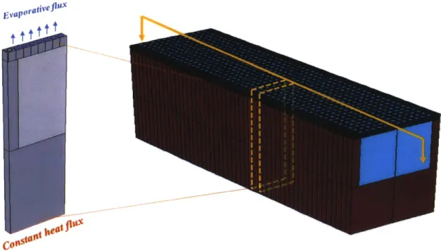
We already know that heat conducts through the channel walls, spreads through the membrane and goes across the liquid to liquid-vapor interface where evaporation occurs. Considering the periodic feature of the structure in this device (Figure 3), we can take one slice of the device as a unit working cell. We include part of the substrate in our thermal model to take into account the constriction resistance. A uniform heat flux is applied to the bottom. The lateral boundaries are assumed to be adiabatic. Still, we need more information about the evaporative flux on top. Similar to the pressure drop problem, we need to first solve for the pore-level transport which can serve as a non-linear boundary condition for the device-level model. In this way, we can bridge the gap between different scales. However, before that, the more general problem, the one-dimensional steady state evaporation problem, needs to be re-investigated

Evaperativef"

Figure 3 One working unit of the cooling device: periodic boundary conditions are applied to the lateral walls, a constant heat flux is applied to the bottom of the device and the evaporative flux needs to be adapter from the pore-level transport

3.

INTERPHASE MASS TRANSFER

A more general problem of evaporation is the steady state evaporation from half-space liquid into

half-space vapor at a steady state, which serves as a boundary condition of the pore-level transport. 3.1 PROBLEM FORMULATION

Vapor f f+

Gas dynamic region

uz

U0

Evaporation

Knudsen layer I &f~ 9f+ t

Liquid v Interfice

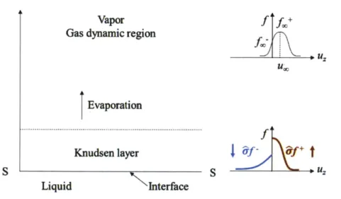
Figure 4 Formulation of the one-dimensional steady state evaporation from half-space problem: the vapor flow is first of very high non-equilibrium and then relax itself to reach Euler equilibrium

Figure 4 describes the vapor flow structure near the evaporating surface (S). To simplify the problem, we assume ideal gas behavior in the vapor phase. The temperature of the condensed phase surface is assumed to be T while the far field vapor temperature is assumed to be T.. We denote P as the pressure of vapor that is in equilibrium with the liquid phase. Very close to the liquid-vapor interface, within the so-called Knudsen layer [19], the vapor flow is highly non-equilibrium and the velocity distribution function (/) differs much from the non-equilibrium case. At a certain point in the evaporation space, the vapor molecules relax themselves to reach Euler equilibrium where the velocity distribution can be described using the Maxwellian distribution with a drift of the bulk vapor velocity u.:

ex

_ x d[UX 2+ U, +(UZ _U..)2 1

2

djo 2R T

f---(2

P. (21rRT )3/2

where p. is the vapor density in the far field, and ux, uy and uz are the molecular velocity in x, y and z directions respectively. At this time, we first denote the vapor velocity distribution function at the interface as

f

3.2 PREVIOUS APPROACH

The most commonly used assumption can be traced back to Schrage's work in 1953 [20]. Schrage assumed that the vapor molecules that are directed back to the liquid-vapor interface follow the velocity distribution of the negative part of the velocity distribution in the far field, i.e.,

f

Then by conserving mass flux between the far field and the evaporating surface, the interfacial flux is derived as a function of the pressure and temperature both in the far field and at the evaporating surface (four parameters). However, recent studies [19, 21, 22] have shown that in this derivation, only mass conservation has been considered while momentum and energy

conservation are not allowed, which makes the approach inconsistent. On the other hand, numerical studies [23] of the Boltzmann Transport Equation (BTE) which governs this transport problem have shown that the evaporative flux is a function of only three of the four parameters of the system (the pressure, and the temperature both in the far field and at the evaporating surface). In other words, Schrage's approach over-constrained this one-dimensional steady state evaporation problem.

3.3 CURRENT APPROACH

The main aspect that Schrage did not take into account is the highly non-equilibrium state of the vapor near the interface which consists of two opposite flows of molecules. We denote 6 as the accommodation coefficient which denotes the portion of incident vapor molecules that will condense into the liquid phase. We assume that the portion of excited liquid molecules that will

leave the interface is also a^ and for the purpose of this analysis, we take 6 as a constant. Therefore the velocity distribution of emitted molecules is then:

1X (U2 + Y2 2 NZ u, +U, +Z,2 expL " z f =dP- 3n for u, >0 (3) Peq (21rRT)12

where pq is the equilibrium vapor density that can be determined from Pq and T. As to the vapor molecules directed back to the interface, we approximate the distribution function using the same approach as in [19]:

ux

U.2 + u,2 + {U,- U00)2

d p 2R7T0

= = m - for u < 0 (4)

pf.- (2yrRT. )3/2 f

where p. has the units of density and is an unknown. By conserving mass, momentum and energy respectively while taking into account the evaporation and condensation coefficient, we have:

o a Co Co Co Co

duz du pfouzdu = Jdu, fdu, fipfUzduy

- .0- -.0 _~

_O _0 (5)

0 CO CO(5

+ Jdu~ du~ J6p~fudu,

-Ca

a o o -o

J du, fdu, Jp~foU,2du, = du, Jdu, fp.,fuz2duy

o00

+ Jdu~ du~ Jdpfu2du,(6

C C

0 2+ 2+ 2 002 2+ 2

Jdu, Jdu, fp~of~ouZ X Z du, = du du, J fu X '

2 ~

fX

- -0 - 0 -CO -22 (7)

0 00 Go2 2 2

+ f duf du+ +fuU du

-- Go -. 00 -. 00 2-C0 --G o - C o eq2Y 7

From the three equations above, we can solve for the three unknowns (uo., poo and p.) which complete our knowledge about the vapor phase. This moment method of solving non-equilibrium flow shows satisfactory agreement with numerical solutions of the BTE [21].

Figure 5 plots the interfacial flux as a function ofthe temperature ratio from the evaporating surface to the far field for three different fluids (octane, water and pentane evaporating into its own vapor at 300 K). The heat flux increases sharply with the interface temperature as the molecule emission

intensity increases. One might think water is certainly the best fluid in terms of heat dissipation because of its large latent heat value and this explains why water has a higher heat flux than octane. However, what is more important than latent heat in this case is the energy density or the product of latent heat and vapor density. Water vapor has a very low saturation pressure which corresponds to a very low density compared pentane vapor which has a very high saturation pressure. This explains why pentane has a larger interfacial heat flux than water. In the following analysis, we continue to use water as an example fluid to illustrate how the overall model framework works.

45 LL 40- Octane --- Water 5 --- Pentane 35- 30- E25-Cr15 - 10-1 1.02 1.04 1.06 1.08 1.1 1.12 1.14 1.16 1.18 1.2 T/T 3000

Figure 5 Interfacial heat flux as a function of the temperature ratio between the evaporating surface and the far field vapor for three different fluids (octane, water and pentane)

Besides the working fluid, another parameter that might influence the interfacial transpo rt is the

accommodation coefficient. For water, most experimental studies indicate that the accommodation coefficient is much less than I (~ 0. 1 or 0.0 1), which means the molecular exchange at the interface is not of high intensity. This contrasts with molecular dynamics studies which give results that are

close to unity. We will elaborate further on this effect of the accommodation coefficient in the pore-level transport chapter.

3.4 SUMMARY

We have investigated a one-dimensional steady state evaporation problem. Inconsistencies in the previous mass conservation based derivation have been addressed and an alternative solution method has been suggested to mitigate the irregularities of past work. The moment method of solving BTE has been adapted to relax the over-constraints of previous derivations and shows very good agreement with numerical studies. The interfacial heat flux has been shown to be a function of the interface temperature and the effect of the fluid properties are very important to the resultant heat flux. More importantly, the power density in the vapor phase rather than the latent heat of the fluid has been proposed as a critical criteria when choosing the best fluid for heat dissipation.

4.

PORE-LEVEL TRANSPORT

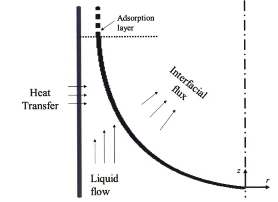
Evaporation from nanostructures is of fundamental interest since sub-continuum transport and intermolecular interactions become relevant at such scale. Previous studies [24-28] that model evaporation from a pore generally follow the framework developed in [28]. The augmented Young-Laplace equation [27] on the liquid-vapor interface was solved together with the fluid mechanics and heat transfer inside the liquid domain. In Figure 6, heat flux go through the pore wall, across the liquid and then arrives at the liquid-vapor interface where it is taken away by the vapor and the fluid flows through the pore to reach the evaporation site.

Heat

Transfer

Liquid

flow

Figure 6 Previous approaches that model evaporation from a pore: the heat transfer and fluid mechanics are solved in the liquid phase assuming that the meniscus is fully extended (dr/dz = 0) at the joint of the adsorption layer and evaporative meniscus) and the interfacial flux can be calculated by

Equation 8.

Note that there are two assumptions built in this kind of approach. First, the meniscus is parallel

is not necessarily the case when the meniscus is pinned at the top of the pore. Second, the mass flux on the liquid-vapor interface can be calculated by Equation 8 [20].

2

1

r 2 =

Ji-i*

2-^ 4 2 rR RT J; r RT

where the evaporation coefficient and the condensation coefficient are assumed to be equal (to 6), Peq is the pressure of vapor in equilibrium with the liquid, T is the temperature of the evaporating surface, P. and T. are the pressure and temperature in the far field respectively, and R is the gas constant of the vapor. Equation 8 (or even its more general form which has a bulk vapor velocity correction factor [20]), however, considers only mass conservation and does not allow momentum and energy balance. It diverges considerably with numerical solutions of Boltzmann Transport Equation [21]. Moreover, this expression fails to include the sub-continuum feature ofthe transport when the pore size comes down to hundreds of nanometers.

4.1 PROBLEM FORMULATION

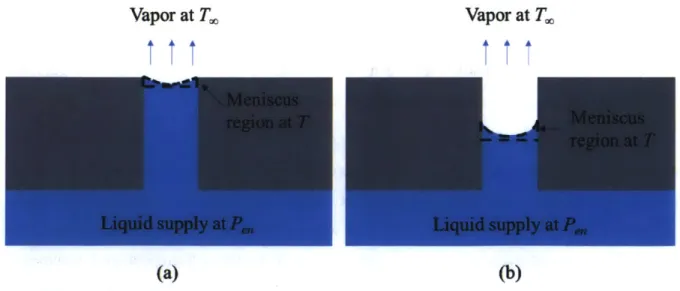
In the present study, a new model framework has been developed to address the above issues. We model a cylindrical pore in contact with a liquid supply on the bottom and exposed to the vapor phase on top as shown in Figure 7 (a) and (b).

Vapor at T,,, Vapor at T.

(a) (b)

Figure 7 A nanopore is exposed to a vapor ambient on one side and on the side in contact with the

liquid phase that wets the pore wall. The pore system falls into different working regimes under different operating conditions: (a) meniscus pinned at the top of the pore and (b) meniscus that recedes inside the pore.

We consider the case that the liquid wets the pore of which the diameter is on the order of 10

-100 nm. Assume that the far field vapor temperature is given as T.. Without losing generality, we

prescribe the liquid entrance pressure Pen at the pore inlet and the average temperature T of the meniscus region which we defined as the liquid above the horizontal plane cutting through the center ofthe meniscus (the dash region in Figure 7 (a) and (b)). Those parameters mark the working condition of this microscopic system. They are in reality often coupled and can be iterated with the macroscopic fluid mechanics and heat transfer. In the present work, we are interested in the steady state evaporative flux over the pore area as a function the prescribed parameters for a given pore geometry.

As the operating condition varies, this pore system may work in different regimes. We shall consider only the case that the liquid pressure is less than the vapor pressure on the interface, otherwise the liquid may flood the top surface of the pore. When the pressure difference across the interface is relatively small, the meniscus tends to be pinned at the top as shown in Figure 2 (a). In the pinning regime, the meniscus responds to different working conditions by changing the interface shape. When it is fully extended (which past work assume to always be the case), the meniscus holds the maximum interfacial pressure difference. If we further reduce the liquid entrance pressure or increase the working temperature that point, the meniscus will recede into the pore as shown in Figure 2 (b). In the receding regime, the interface keeps the same shape while moving up and down inside the pore. In this way, it changes the viscous loss in the liquid phase to maintain the pressure difference across the interface. If the interfacial pressure difference is still too large for the meniscus to hold even when the meniscus recedes to the bottom of the pore, the vapor will expand into the liquid supply and the pore system will dry out.

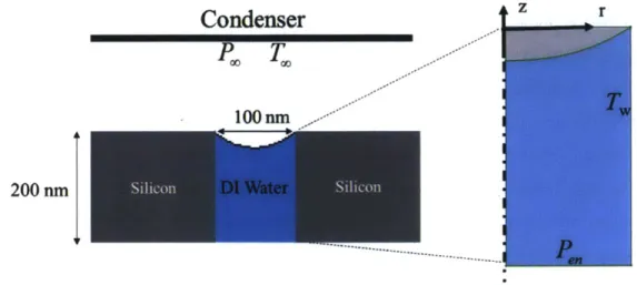
For our analysis, a heat flux (q") on the order of 1 kW/cm2 is considered since this work is a benchmark case. In Figure 8 we chose a fixed pore diameter of 100 nm and a pore length of 200 nm in this study, which can result in a high capillary pressure (- 2 MPa for water) while minimizing the viscous loss. Deionized water is considered as the working fluid and the pore wall is assumed to be silicon, which has a relatively high thermal conductivity such that the wall temperature is assumed to be uniform (Tw). We set the condenser temperature and pressure to be fixed parameters based on the desired operating conditions. Specifically, in this study T. = 300 K and P. is the saturation pressure

are two local variables which determine the interfacial transport. We sweep the parametric space

of Pen and Tw to understand the dependence of the interfacial heat flux and heat transfer coefficient

on these two governing parameters.

Condenser

P

T

100

nm

200 am

...

Figure 8 Schematic of each domain, showing the model inputs and the cylindrical coordinate system; the pressure and temperature at the condenser (P. and T.), and the pore geometries (radius and length) are predefined parameters.

In the pinning or receding regime, we evaluate the effects of temperature and pressure variance inside the meniscus region by plugging in properties of liquid water and taking heat flux as " = 1 kW/cm2, pore radius as rpore = 50 nm, the reference temperature as T = 300 K. Then relative temperature variance within the meniscus region can be estimated as q"rpore/kiT « 1. Hence, the interfacial transport will not be significantly influenced if we neglect this temperature variance.

The pressure variance APL in the meniscus region can be approximated as pirh/2r3ore. This results in a change in the equilibrium vapor pressure APeq/Peq = exp[AP1/(pjRT)] - 1 « 1.

Additionally, this pressure variance contributes very little to the interfacial pressure difference, APu1/APn < 1 which implies that the meniscus shape is not sensitive to the viscous

loss in the meniscus region. Therefore, the variance of pressure inside the meniscus region does not have much impact on either the intensity of molecule emission on the interface or the apparent evaporation or condensation coefficient.

4.2 MODEL DESCRIPTION

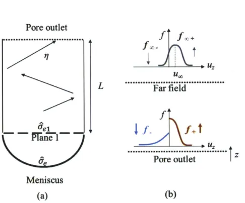
In order to model the interfacial transport inside a pore, we need to couple the vapor transport, liquid transport and the interfacial balance. Outside the pore, we can well model the molecular transport using the moment method. For the transport process inside the pore, we assume that the vapor is in the free molecular regime since the characteristic length (- 100 nm) is less than 10%

of the mean free path in the vapor phase (- 1.1 gm). We shall first investigate the probability of a

liquid molecule being emitted from the interface and escaping the pore as well as the probability of a vapor molecule condensing onto the interface after reaching the pore outlet. We follow a similar approach developed in [29] assuming free molecular vapor flow inside the pore. In Figure 9, we imagine a virtual horizontal plane (Plane 1) right on top of the meniscus. Considering the evaporation case, the probability of a liquid molecule at the interface to go across Plane 1

(Uei)

61iA, Am

where A, is the cross-section area of the pore and Am is the surface area of the meniscus. On the other hand, the transmission probability of a molecule through a pore has been calculated in [30] under the free molecular flow assumption:

[2 (2 4*272+4+L73-16]2

S17 + -CL+ ( 7 (10)

4 4 _L+472+4

7 2 f42+4- 2 88 nL ( 2

where the reduced pore length L* is defmed as the dimensional pore length over the radius. Note that a molecule can be directed back to the interface from the pore wall and then reflected, but it has to go across Plane 1 an odd number times for it to eventually escape the pore. Let's define E, as the probability of a liquid molecule at the interface to reach the pore outlet after going across

Plane 1 2n - 1 times (n = 1, 2, 3 ... ). Then En+1 can be related to En as:

Pore outlet ... f f OC. L

Far field

Figure 9 Vapor transport in the pore system: (a) emitted molecules first reach Plane I with a probability 6

e1 and the transmission probability from Plane I to the pore outlet is 11; (b) vapor transport

outside the pore with the far field vapor in Euler equilibrium and the near interface vapor velocity distribution.

It is obvious that El = 6 i7 and {E,} is a geometric sequence. Then the apparent evaporation

coefficient from the pore outlet or the overall probability of a liquid molecule being emitted from the interface and escaping the pore can be calculated as:

E qA

=2E,, - 1 - (12)

n= _

1-(1-_)(1-&,) 7(1-_)A, +A(,

Note that the interfacial transport takes a great hit as the meniscus recedes inside. Therefore we would like to keep the meniscus pinned at the top (I = 1).

In order to determine the overall cooling performance, the shape of the evaporating interface is first investigated. We use a cylindrical coordinate system with the origin set at the center of the meniscus, as shown in Figure 8, to derive the governing equations at the interface.

Due to the small pore, the vapor pressure on the interface (Pri) is expected to be uniform. The

where usat is

gas constant

Psat+ RT In = Psai + (p '

Ja) (13)

Psat P, /M

the chemical potential corresponding to the saturation state. R denotes the universal and M is the molar mass.

t

Evaporative

flow

No-slip

Entrance

pressure

Figure 10 _{Boundary conditions for (a) liquid-vapor interfacial pressure balance and (b) liquid} transport inside a pore

The variation of liquid pressure on the interface is then also negligible according to Equation 13. Meanwhile, we consider the normal stress balance at the interface as follows:

P, - P1 = 2o7c+]Fd (14)

The interfacial pressure difference consists of two parts in Equation 14: the first term arises from

the curvature of the interface (K), signifying the surface tension effect. The second term, the

disjoining pressure Lid is given in [25, 26] as

fl~r> 0 (,rkBT) -A

21 ( = + 3 (15)

2(r,,re -r )K Ze 6 (r,, -r)

where E is the dielectric constant, EO is the vacuum permittivity, kB is the Boltzmann constant, Z is the number of charge per ion and e is the elementary charge. The first term in Equation 15

in traditional models [28, 31-33] and the second term is the van der Waals interaction which is evaluated with a non-retarded Hamaker constant A [34] between the solid (Medium 1) and the vapor (Medium 3) across the liquid (Medium 2).

3 = -__, 3hV, (2 )( n2 n22

A =-kBT _{+ (16)}

4 s+6, 8 n, +n n +n n + + +

This expression of disjoining pressure will encounter a singularity at the pore wall and the existence of an adsorption layer eliminates this singularity. The thickness of the adsorption layer can be approximated by setting the local evaporation rate as zero. The calculated adsorption layer thickness is less than 1 nm following Equation 17.

Pr - ,pRTIn I+P = +(

Pt ) rpr -6 6)r 3

where the LHS is the pressure difference between the vapor and the liquid in equilibrium with it (from Equation 13). When the interfacial pressure difference is relatively small, Equation 14 can be integrated from r = 0 to r = rp - 5. The maximum pressure difference that the meniscus can

hold can be evaluated by adding another constraint (dr/dz = 0 at r = rp- 8). Since the system is

not at equilibrium, Pi does not equal to the equilibrium vapor pressure but can be iterated with the vapor transport. Right at Plane 1 in Figure 9(a), the number density in the vapor phase is

00 00 GO0000

p1= du, fdu,, Ja-,pfdu,+(1+I-& ) du dux pfdu, (18)

0 -.0 -c - --W -c

The RHS includes the molecules being emitted, directed back and being reflected, all evaluated at Plane 1. Then we can balance the mass and momentum flux between Plane 1 and the far field:

Go C0 00

plu = fdu- Jdux f p fwuzduy (19)

-.00 -- 0 -.00

00 00 00

p +P = du dux fpfudu (20)

--00 -00 -00

where ui is the bulk vapor velocity at Plane 1.

In the liquid domain, we assume a steady, incompressible and axisymmetric flow. The bulk liquid

velocity (Vi) is approximated by energy conservation: V~ q"/ (hfgpi), where hfg is the enthalpy of vaporization of water, and pi is the density of liquid. Therefore, the Reynolds number in the liquid phase can be expressed as:

Re, = VD 10-3 (21)

P,

where D is the pore diameter. Due to the low Reynolds number, the liquid flow inside the pore is in the laminar regime. The governing equation for the balance of linear momentum is then given as:

pu-Vu=-VP+pV 2u (22)

where the unsteady term and body forces are neglected. The pore inlet pressure is set as the boundary condition, Pen. While the liquid is transported to the interface and evaporates, the temperature gradient along the interface can potentially induce Marangoni convection. Buffone and Sefiane [35, 36] reported that Marangoni convection can play an important part when evaporation occurs inside a micro-scale capillary tube. For the dimensions of interest in this study, we can estimate the temperature difference inside the liquid domain considering the heat conduction: AT - (q "/ ki )L, where ki denotes the thermal conductivity of the liquid and L is the characteristic length of the problem domain. The Marangoni number is then calculated as

dcaLAT

Ma = - (23)

dT p,a

where a denotes the surface tension, pi is the liquid dynamic viscosity and a is the thermal diffusivity of the liquid. The calculated Marangoni number (- 5) is less than 80, which suggests that the Benard-Marangoni instability is not likely to occur.

At the liquid-vapor interface, mass conservation results in the following equation which equates the liquid mass flow rate to the interfacial vapor mass flow rate in Equation 19 (a). Liquid flow is also coupled with the overall heat transfer through the convective term in the energy conservation equation:

p,cpu -VT =V -(kVT) (24) In order to determine the boundary conditions for heat transfer, the liquid inlet is assumed to be adiabatic and the pore wall is assumed to be maintained at a constant temperature (T.). At the interface, the evaporative heat flux is equated to the heat flux due to heat conduction in the liquid.

nguivedn Receding YesM No p Yes ()tree interReceding balanoe ? transpo.No No

Gie an a cYes ph _dmene

Receding L

o e ad conv er tw

No

L

(b)

Figure If Computational flow chart to solve for the flux across the pore system: (a) test if the system goes beyond the pinning regime and iterate around liquid and vapor pressure at the interface, Pli and Pvi (b) iterate around the reduced length L if the system is in the receding regime.

Given an operating condition ofthis por weEqution are then able to determine the working regime

and calculate the flux across it. We initialize the computation by setting Pli the same as P,., and P,, the same as Pt (T.). As shown in Figure I l(a), we first test if Equation 14 on the interface is

convergent around the adsorption layer to determine whether the meniscus will recede. If the pressure difference is more than what the interface-can hold, then we reach the receding regime. If not, we still stay in the pinning regime and an interface shape can be calculated. Then with the help of vapor transport analysis, we can recalculate Pyi. If it converges to the previous value, then we can plug the mass flow rate into the Equation 20 to recalculate Pii If this also converges, then

the transport problem in the system is solved in the pinning regime. If the convergence is not reached, we keep iterating around Pi and P1. In the receding regime (Figure 7(b)), since the

meniscus is fully extended, the interfacial pressure difference and the meniscus shape are both known. Then for a given receding length (L), the interfacial transport is determined and Pu can be calculated from the vapor side. Also, PJi is related to L via the liquid transport. Therefore, we can iterate around L to solve for the interfacial transport in the pinning regime as shown Figure 7(b). The relative tolerance and convergence criterion during the computation is set as 1 x 10-4

10 1 110 T-T.,, =20K,6= 1 T - T = 10 K,8 = 1 10 0 (kW/cm2) z (nm) -20 10 10'T - T. =20 K, =0. 1 -30 10 -2 T -T,, =_107 = 0.1t--- -40--4 -1 0 0 10 20 30 40 50 P. (MPa) r (nm) (a) (b)

Figure 12 (a) Pore-level heat flux normalized over the pore cross-section area as a function of the entrance pressure for selected superheats and accommodation coefficients. (b) The shape of meniscus for selected entrance pressures at 20 K superheat with accommodation coefficient of 0.1

Using this computational strategy, we able to solve for the pore-level transport. Figure 12 (a) plots the pore-level heat flux normalized over the cross-section area of the pore as a function the entrance pressure for some selected superheats and accommodation coefficients.

Since the liquid is supplied to the pore passively via capillarity, we expect negative pressure under the pore, i.e., at its entrance. When the entrance pressure is too negative, the meniscus cannot hold the pressure difference across the interface and the interface recedes into the pore and the system dries out. Before the dry-out, the interfacial heat flux is enhanced for a higher value of superheat or for a higher accommodation coefficient as we expected. In addition, when the accommodation coefficient equals one, the heat flux remains unchanged as the entrance pressure decreases. However, when the accommodation coefficient is 0.1, as the entrance pressure decreases the heat

flux gradually increases which can be explained by the meniscus shape change. Figure 12 (b) plots the interface shape for some selected entrance pressures. The meniscus extends itself to generate more capillary pressure as the entrance pressure decreases. This extension of the interface gives rise to more surface area for evaporation and thus enhancing the interfacial transport. To understand this, consider a radiation analogy, where for a gray body, the more surface area, the higher apparent emissivity (the accommodation coefficient less than 1), however when it comes to a black body (the accommodation coefficient equals 1), the surface area is not relevant.

8 =1 100 4" B 0.5 (kW/cm2 ) 10 8 0.1 T - T .(K)

Figure 13 Pore-level heat flux as a function of superheats for selected accommodation coefficient In reality to maintain a stable operating mode, we would like to operate a cooling system designed around this pore model where the heat flux is insensitive to the entrance pressure or in Figure 12 (a) where entrance pressure is greater than -1 MIPa. In this regime, the pore-level heat flux is only a function of temperature as shown in Figure 13.

It is also indicated in Figure 13 that the pore heat flux is highly dependent on the value of the accommodation coefficient. The understanding of this parameter is still at an early stage [37] and it will be our future work to do theoretical modeling and experimental characterization of this parameter.

4.4 SUMMARY

A more consistent model has been developed for the heat and mass transfer near a meniscus inside

a nanopore. A more accurate description for vapor transport has been adapted to calculate the interfacial flux and recondensation inside the pore has been considered. The laminar flow, heat transfer and vapor transport problem were all solved in terms of the local temperature and the liquid supply pressure. The interfacial heat flux constantly increases with the local pore wall temperature and is also highly dependent on the pressure at the pore entrance when it is relatively low. The current pore-level model relates the nano-scale transport to macro parameters and can serve as a non-linear boundary condition to the device model which is discussed in the following chapter.

5.

DEVICE PERFORMANCE MODEL

For electronic cooling applications, the dependence of temperature drop on can be used to manage the temperature at hot spots independently from background heating zones. Without a heat spreader, large maximum lateral temperature change will be expected. Only with an embedded thermal management approach that can be customized to cool hot spots independently from background regions can the traditional thermal stack of heat spreaders and thermal interface materials be eliminated, thereby significantly improving thermal dissipation in advanced electronic devices.

Now that we have modeled the interfacial transport, we have enough boundary conditions for the cooling device which can mitigate this spreading problem. For a given design, we can calculate the pressure drop in the microchannel and make sure that the heat flux does not fluctuate much with the entrance pressure. To model the heat transfer performance, we applied the function graphically described in Figure 13 as a non-linear boundary condition for the evaporative flux in Figure 3.

5.1 CASE STUDY

We fix the flow length in the micro channel to be 100 gm, which makes this concept ready to scale up. We can vary the channel width, channel height, as well as the membrane parameters (pore radius, porosity and membrane thickness) as shown in Figure 14.

Membrane (porosity, pore radius)

Figure 14 Geometric parameters in the cooling device that we sweep in the optimization process including the membrane geometries (porosity, pore radius, thickness) and microchannel parameters (height, wall width and spacing)

As a reference case, we first study the parametric set where rpore = 50 nm, porosity = 0.27, tmem =

200 nm, h = sp = 2 pm, and w = _{400 nm. We set the vapor temperature in the far field at 323.15 K} and set the heat flux as 1 kW/cm2

based on our application of cooling electronics [38]. Since we would like to keep the meniscus pinned at the top and relatively flat to have less fluctuation with regard to the pressure under the membrane, the pressure drop inside the pore can be calculated using the Hagen-Poiseuille equation and the pore-level transport can be equivalently modeled as an evaporating flat interface. This allows us to study pentane as the working fluid which has the best heat transfer performance. It is important to note that for a much extended meniscus, the pentane vapor inside the pore is in the transitional regime which is between the continuum regime and the free molecular regime and very complicated to model. To verify the accuracy of using this model for the given case study with pentane, we calculate the total pressure drop using Equation 1 to be 0.45 MPa. Since the total capillary budget is ~ 0.72 MPa for a semi-spherical interface, this indicates that the meniscus will be pinned at the top and almost flat, which is consistent with the assumption that we have made and hence validates the use of the model with pentane. In terms the

heat transfer, the temperature rise of the substrate with uniform heat flux was modeled using

COMSOL Multiphysics TM _{finite element analysis.}

Temperature ('C) S80.374 so 78 76 74 72 70 68 66 F 63.78

Figure 15 _{Temperature profile from COMSOL model of the reference case with the applied heat flux} q = 2 kW/cm2_{. Heat is conducted from the substrate, through the ridge, and to the membrane pores where}

liquid evaporates. The heat conduction and convection in the liquid is insignificant compared to conduction in the ridge.

The solution was found to be independent of the grid size above 379 elements. Due to the symmetry of the structure, the problem can be reduced to a control volume which contains the ridge, ridge channel and membrane as shown in Figure 14. From the thermal model, the heat convection and conduction in the liquid is insignificant compared to conduction in the ridge. Therefore, any cross section has the same temperature profile and it can be assumed that the front and back faces are adiabatic. The left and right faces are adiabatic to represent mirrored conditions while the front and back faces are adiabatic to represent repeating boundary conditions. The liquid interface in the pores is assumed to be flat in the thermal model and evaporation from the pore surfaces is approximated by the pore-level transport part. Thermal conductivity values of Si were assumed equal to bulk values (k=130W/m-K) except in the ridge and membrane where values of

k=63 W/m-K and k=60 W/m-K were applied, respectively, to reflect non-continuum heat transfer

in microstructures. An example temperature contour plot of the model domain is plotted in Figure

15, where there are significant temperature gradients both vertically in the microchannel walls,

laterally in the membrane and within the liquid in the membrane pores indicating that all of these geometries are important in determining the overall thermal resistance of the evaporator. Additionally, there is a significant temperature change associated with phase change (13.78 K). The liquid evaporates from the pores into a pure vapor environment; therefore, there is assumed to be no temperature change associated with convection of vapor. After evaporating from the pore surface, the vapor flows as a pure substance to an external condenser maintained at a desired temperature. The thermal resistance of the condenser is not considered here.

5.2 PARAMETRIC SWEEP

To better understand the influence of the membrane and ridge geometries on temperature drop, we conducted a parametric sweep of the membrane thickness (tmm), membrane porosity (p), ridge thickness (w), and ridge channel width (sp) and then studied their influence on the total temperature and pressure drop. The ridge channel width is coupled to the height (h=sp) and the heat flux is fixed at 1 kW/cm2

. The results are shown in Figure 16 and Figure 17 with the temperature

+=0.108 ---. =0.272 0.09 25- ..-.----....-- +=0.46 -0.08 20--0.07 0- 15-- 0.06 1900 1M . O M M 5

Msmranre ttickness (run)

Figure 16 Temperature drop and pressure drop as functions of membrane thickness and porosity. The ridge height and spacing are 2 pm while the microchannel width is 0.4 pm.

40 0.3 tr=0.2 pm --- t=0.4 pm ... tr=0.8 pm 35 0.2 30 0.1 20 r r r r r 0 0.5 1 1.5 2 2.5 3 3.5 4 4.5 Ridge Width (pm)

Figure 17 Temperature and pressure drop as a function of ridge channel width and ridge thickness. The membrane porosity is fixed at porosity = 0.272 while the membrane thickness is fixed at 200 nm. The trends in Figure 16 indicate that a more porous membrane is always desirable to minimize both temperature and pressure drop in the device. Additionally, a thin membrane is better for

pressure drop and has only a small influence on temperature. In Figure 17, there is an optimum value for the ridge channel width with respect to temperature drop while the pressure drop increases dramatically when the ridge channel is reduced below 2 pm. Although these plots are helpful in revealing trends for various device geometries, a more useful plot for identifying a global optimum set of values is shown in Figure 18 where the total temperature drop is plotted with the excess pressure drop, i.e. the difference in capillary pressure and viscous pressure drop. The only relevant solutions in the plot for a passively pumped evaporation device are in the upper left quadrant where the temperature drop is less than 30 K and the excess pressure drop is positive. Among these solutions, we choose one set of geometries with the highest excess pressure and lowest total temperature drop:

5-0 -15- I -2

-2

Figure 18 Summary of temperature (AT) and excess pressure drop (APp - AP,) for all ridge and

membrane geometries. Only solutions with a positive excess pressure and temperature drop less than 30 K (highlighted quadrant) are feasible.

The model results for temperature rise using the optimized values and variable membrane porosity for three different values of heat flux are plotted in Figure 19. As the porosity increases, more surface area is available for evaporation, therefore the interfacial resistance decreases. The waviness in the data is a result of discretization of the number of pores that fit into the domain of the model. The current design of membrane and ridge geometries is predicted to dissipate 5

Although thermal resistance continues to decrease with increasing porosity, the improvement diminishes at higher porosity because of the reduced thermal conductivity of the porous membrane and fixed thermal resistance of the ridge structure. Additionally, limits in fabrication will eventually be reached as the mechanical integrity of the membrane deteriorates with an increase in porosity. 70 A A * q kW/cm 2 60 A A A q 2 kW/cm2 A _{A g =q5kW/cm}2 50-A 40 * A AAA A AA 1 0-0.1 0.2 0.3 0.4 0.:5 Porosity,

#

Figure 19 Temperature rise in substrate vs. porosity for hotspot heat flux of 5 kW/cm2 (gray curve), intermediate heat flux of 2_-kW/cm2 (orange curve) and background heat flux of I _kW/cm2 (blue curve).

If a membrane porosity of =0.5 is used over the hot spot and =0.1 over the background, the heated

regions experience a temperature rise of less than 30 K from ambient vapor while the difference between them is less than 10 K (highlighted area).

For electronic cooling applications, the dependence of temperature drop on can be used to manage

the temperature at hot spots independently from background heating zones. An example is shown

in Figure 19 in which a low porosity (# =0.1) membrane is applied to the background

(q=1 kW/cm2) while a high porosity (0 =0.5) membrane is applied to the hot spot (q=5 kW/cm 2). In this way, the temperature rise in the hot spot and background are kept below 30 K while the lateral temperature difference is less than 10 K, ensuring reliable operation of the semiconductor

junctions.

approach that can be customized to cool hot spots independently from background regions can the traditional thermal stack of heat spreaders and thermal interface materials be eliminated, thereby

significantly improving thermal dissipation in advanced electronic devices. 5.3 SUvMARY

A membrane based heat dissipation device was designed considering the pressure drop associated

with its microfluidic supply channels and thermal resistance of the membrane and support structure. A finite element conduction and evaporation model was developed to estimate the results temperature drop across the device while an analytic model was used to estimate the pressure drop.

A parametric sweep of critical geometries in the membrane and ridge demonstrate the sensitivity

of performance to each metric. The analysis demonstrates an upper bound for high heat fluxes that can be dissipated by a silicon device with supported membrane and with a substrate-to-ambient temperature difference of less than 30 K.