New Brunswick hydrometric network analysis and rationalization.

New Brunswick Hydrometric Network Analysis and Rationalization

Alida Nadège Thiombiano4 8

1. Department of Civil Engineering, Université de Moncton, Moncton, N.B., Canada. 9

2. Department of Mathematics and Statistics, Université de Moncton, Moncton, N.B., Canada. 10

3. Fisheries and Oceans Canada, Moncton, N.B., Canada. 11

4. Centre Eau–Terre-Environnement, Institut National de la Recherche Scientifique, Quebec Canada 12

13 14 15

*Corresponding author: Nassir El-Jabi, Department of Civil Engineering, Université de Moncton, 16

Moncton, N.B., E1A 3E9, Canada, 17

Telephone: (506) 858-4296; Fax: (506) 858-4082; E-mail: Nassir.el-jabi@umoncton.ca 18

19

Word Count : 8397 20

Abstract

The availability of hydrometric data, as well as its spatial distribution, is important for water

22

resources management. An overly dense network or an under developed network can cause

23

inaccurate hydrological regional estimates. This study's objective is to propose a methodology

24

for rationalizing a network, specifically the New Brunswick Hydrometric Network. A

25

hierarchical clustering analysis allowed dividing the province into two regions (North and

26

South), based on latitude and high flow timing. These groups were subsequently split separately

27

into three homogeneous subgroups, based on the generalized extreme value (GEV) distribution

28

shape parameter of each station for annual maximum flow series. An entropy method was then

29

applied to compute the amount of information shared between stations, ranking each station's

30

importance. A station with a lot of shared information is redundant (less important), whereas one

31

with little shared information is unique (very important). The entropy method appears to be a

32

useful decisional tool in a network rationalization.

33

Keywords : hydrometric network; GEV; clustering analysis; entropy ranking; New Brunswick

34

Résumé

La disponibilité des données hydrométriques ainsi que la distribution spatiale des stations

36

hydrométriques sont d'une grande importance pour la gestion des ressources en eau. La

37

couverture spatiale est souvent très faible, ce qui peut causer des simulations hydrologiques

38

inexactes. L'objectif de cette étude est de proposer une méthodologie pour la rationalisation du

39

réseau hydrométrique du Nouveau-Brunswick. L’approche proposée combine une méthode de

40

classification basée sur le comportement des extrêmes hydrologiques et une mesure de

41

l’information conjointe produite par l’ensemble des stations disponibles dans le réseau. Une

42

approche de classification hiérarchique a permis de diviser la province en deux secteurs dits

43

homogènes (Nord et Sud) en fonction de la latitude et de l’occurrence des débits maxima

44

annuels. Chacun de ces groupes a été divisé en trois sous-groupes homogènes, selon la valeur du

45

paramètre de forme de la distribution GEV des débits maxima annuels de chaque station. Une

46

méthode basée sur l'entropie a permis le classement des stations en fonction de leur importance

47

dans leur groupe respectif (Nord ou Sud), en calculant la quantité d'information conjointe entre

48

les stations. Ainsi, une station qui comporte beaucoup d’information commune avec d’autres

49

stations est considérée redondante, et donc moins importante. Une station avec très peu

50

d'information partagée est considérée unique, et donc très importante. Le classement des stations

51

par ordre d'importance peut être un outil décisionnel utile. Les stations ont été ordonnées selon

52

leur importance, et la méthode d'entropie se présente comme un outil décisionnel utile dans la

53

rationalisation du réseau.

54

55

1. Introduction

The importance of hydrometric gauging station networks for surface water monitoring is well

57

established, given the usefulness of collected hydrometric data for decision making related to

58

water resources management around the world (Hannah et al. 2011). However, the density of

59

these networks is still being impacted by the shift of social and economic priorities of

60

governments, like that observed in Canada (Burn 1997; Coulibaly et al. 2013; Mishra and

61

Coulibaly 2009). In fact, Pilon et al. (1996) showed that, through the 1990s, data collection from

62

Canadian National Hydrometric Network (CNHN) declined mainly due to financial pressure that

63

impacted the budget of relevant agencies. More recently, Coulibaly et al. (2013) noticed that

64

only 12% of the Canadian terrestrial area, the majority of which is in the southern portion of the

65

country, is covered by hydrometric networks that meet the minimum standards according to the

66

World Meteorological Organization (WMO) physiographic guidelines. Moreover, 49% of the

67

Canadian terrestrial area is gauged by a sparse network and the remaining 39% is ungauged

68

(Coulibaly et al. 2013). Although the negative implications of this may not be immediately

69

apparent, many water resource decisions, project designs and project management rely on

70

information gained by hydrometric gauging stations. In other words, short-comings in a gauging

71

network can lead to greater hydrological uncertainty, which can lead to inefficient project design

72

and resource management, which in turn can have diverse consequences. For example,

73

uncertainty can lead to over-designing, which adds unnecessary extra project costs. In addition,

74

under-designing is also a possibility, which could lead to project failure and extra costs as well.

75

Poor resource management can also impact the population as well as the environment. Although

76

reducing the amount of gauging stations within a network is not ideal according to WMO

77

guidelines, financial and budget restraints may make it necessary. Therefore it seems an

78

evaluation of the network must be undertaken in order to properly analyze options for station

79

reduction or displacement to minimize information loss, thus rationalizing the network. The

80

required assessment must define and integrate appropriate criteria for each region for the

81

network to be properly updated. It is in this context that the present study aims to propose a

82

rationalization of the hydrometric gauging network of New Brunswick (NB). This will be

83

accomplished using a hierarchical clustering analysis and the generalized extreme value (GEV)

84

distribution shape parameter analysis as preliminary evaluation tools of hydroclimatic behaviour

85

and homogeny between gauging stations, and subsequently, with the entropy concept to quantify

86

the importance of each station regarding information content. However, in order to have a more

87

complete rationalization process, data managers and users should be consulted for their input, as

88

other criteria (e.g., quality of rating curves, size of the drainage basin, etc.) may also be of

89

importance in a final decision.

90

Mishra and Coulibaly (2009) provided a review of common methodologies developed to address

91

hydrometric network design or redesign in response to growing management and financial

92

challenges for governments and data users. Using the entropy concept, Mishra and Coulibaly

93

(2010) provided an evaluation of hydrometric network density and the worth of each station, in

94

major watersheds across Ontario, Quebec, Alberta, New Brunswick and Northwest Territories.

95

Their study highlighted the generally deficient status of hydrometric networks, mainly over the

96

northern part of Ontario and Alberta, as well as in the Northwestern regions of Canada. The

97

entropy concept, derived from Shannon information theory (Shannon 1948), assesses the

98

information content of each gauging station of a given network in relation to all other stations of

99

that network. It was adapted to suit hydrological concerns by Hussain (1987; 1989). Its

100

applications showed its usefulness for optimal hydrometric network design in many studies (e.g.,

101

Alfonso et al. 2013; Li et al. 2012; Mishra and Coulibaly 2010; Singh 1997; Yeh et al. 2011).

102

Nevertheless, multivariate analysis methods such as clustering analysis also remain useful

103

statistical tools in the hydrometric network rationalization process. These methods are commonly

104

used to identify homogeny in a dataset, and potentially form groups of similar individuals (in this

105

case hydrometric gauging stations), which is an important step for network rationalization and

106

optimization (Daigle et al. 2011; Khalil and Ouarda 2009). For example, Khalil et al. (2011) used

107

clustering analysis to extract different sub-hydrological units in order to better perform their

108

assessment and redesign of the water quality monitoring network. In hydrology, three parameter

109

distributions are recommended, especially the Generalized Extreme Value (GEV) distribution.

110

Indeed, its statistical properties indicate how the flexibility of this three parameter class of

111

distributions can capture skew and fat tails (El Adlouni et al., 2010).

112

In studies characterizing natural flow regimes, environmental flows and floods in New

113

Brunswick (Aucoin et al. 2011; El-Jabi et al. 2015), it was found that the GEV distribution was

114

an appropriate distribution to model the annual maximum and minimum flows at most of the

115

gauging stations in New Brunswick. For instance, the Anderson-Darling test showed slightly

116

better performances for the GEV than for the 3 parameter lognormal distribution. Unlike the

117

normal distribution that arises from the use of the central limit theorem on sample averages, the

118

extreme value distribution arises from the theorem of Fisher and Tippet (1928) on extreme

119

values or maxima in sample data. The class of GEV distributions is very flexible and its shape

120

parameter controls the size of the tails corresponding to three special cases (Gumbel, Fréchet and

121

Weibull). Therefore, the GEV shape parameter (kappa) is a good indicator of the distribution of

122

the extreme high and low flow events, and thus could be useful in differentiating between

123

different hydrological regimes. Consequentially, it seems that the shape parameter fitted to the

124

annual maximum flow series (GEVkapMax) and the shape parameter fitted to the annual

125

minimum flow series (GEVkapMin) are good for characterising flows in the province. Since the

126

annual maximum flows were particularly well modeled by the GEV distribution, and the

127

maximum flows are generally of more interest, the GEVkapMax was deemed as an appropriate

128

metric to analyze and potentially be used for identifying homogenous groups of datasets.

129

Network optimization cannot be accomplished by solely using these purely statistical

130

approaches, as other factors must be taken into account. For example, a gauging station linked to

131

a hydroelectric facility may not be statistically important in a network, but would most likely be

132

important from a resources management perspective. Data user needs and perception must be

133

integrated in any analysis of a network. It has been recommended and integrated in previous

134

studies (e.g., Burn 1997; Coulibaly et al. 2013; Davar and Brimley 1990). Environment Canada

135

and New Brunswick Department of Municipal Affairs and Environment (1988) investigated

136

accuracy requirements identified by users in order to define a minimum and target networks.

137

They considered mean, low and high flows in this approach, which consisted of developing

138

regional equations for each of the three categories. They initially identified 16 homogenous

139

regions in the province, considering that there should be a small, medium, and large gauged

140

basin in each homogenous area. This implied that 48 stations, plus an additional 6 for larger

141

regions (total of 54 stations), was identified as a minimum network. They also identified a target

142

network, this time considering that 10 stations were necessary per region in order to properly

143

define regional regression equations. However, they also refined the initial 16 homogenous

144

regions into 7 regions. This implied that 70 stations (plus an additional 7 for variations in size)

145

were suggested as the target (total of 77 stations). They concluded that it was important to

146

coordinate hydrographic gauging with meteorological gauging, that more gauging was necessary

147

for smaller catchments, and that the central part of the province lacked gauging stations. They

148

also evaluated the hydrometric network using an audit approach, through which a ranked

149

prioritization of stations was provided based on the hydrometric, socio-economic and

150

environmental worth of each station according to data user perceptions. They also considered site

151

characteristics, economic activity, federal and provincial commitments, special needs, as well as

152

a station's regional and operational users in their audit approach. Davar and Brimley (1990) used

153

a similar approach to identifying a minimum and target network as Environment Canada and

154

New Brunswick Department of Municipal Affairs and Environment (1988), but their audit was

155

slightly different. The existing stations and proposed new stations were evaluated using an audit

156

approach, based on site characteristics, client needs (regional hydrology and operational), and

157

regional water resource importance. They created different scenarios that had different impacts

158

and values (based on audit points) in function of different costs (adding, removing, or

159

maintaining the amount of gauging stations in the network). Overall, their recommendations

160

included: reallocating resources to meet the minimum network; create a committee for ongoing

161

planning and analysis, as well as communication with the user community; emphasize the

162

importance of regional hydrology; coordinate with other related data gathering, such as water

163

quality and atmospheric data. The size of the New Brunswick Hydrometric Network has been

164

subject to change over the years. The network's major expansion occurred in the 1960's, with a

165

peak size of 75 stations achieved in 1978-1979. The network maintained a size of between 69

166

and 72 stations from 1980-1993. In 1994, the number of stations was reduced to 56, a reduction

167

of 22% in the number of stations. By the year 2000, only 46 stations were left active in New

168

Brunswick a further reduction of 14% (i.e., a reduction of 36% compared to the 1980-1993

169

period). This was contradictory to the studies done by Environment Canada and New Brunswick

170

Department of Municipal Affairs and Environment (1988) and Davar and Brimley (1990), which

171

advocated an increase in network size. However, financial pressure required the reduction in

172

gauging station numbers.

173

Due to the fact that network expansion and reduction was mostly done considering site specific

174

needs, as opposed to the network as a whole, rationalization of the network is still relevant in

175

New Brunswick. This study aims to provide a methodology for such a rationalization, and in the

176

case of further budget reductions, a supporting tool for management and decision making.

177

2. Methodology

It should be noted that for all the methods used in this study, the specific discharge (discharge

179

per unit area; m3/s per km2) was used. This was done to remove drainage area as an

180

overwhelmingly dominant variable when it comes to explaining flow rates. In other words, the

181

drainage area was removed as a variable in order to better compare larger basins with smaller

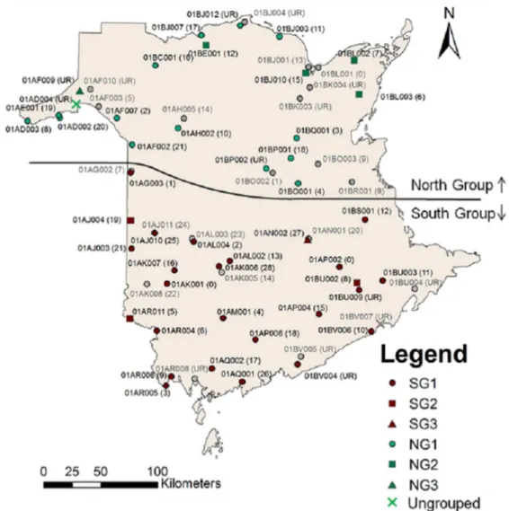
182

basins in terms of flow.

183

2.1 Hierarchical clustering analysis

184

The first approach used in this study was the hierarchical clustering analysis. The objective of

185

this analysis was to divide the province into similar hydrological groups. This was done using a

186

clustering analysis. Thereafter, the GEV analysis further refined these hydrological groupings,

187

and the entropy analysis was carried out in this framework for finer assessment. Rationalization

188

and optimization assessment of the network has been shown to be better conducted with the

189

division of a network into climatic regions (Burn and Goulter 1991; Khalil et al. 2011).

190

The attributes from which similarities will be defined need to be specified for clustering analysis

191

(Burn and Goulter 1991). Once this is done, clusters are formed by grouping similar observations

192

together in such a way that variance is minimized within a cluster and maximized between

193

clusters (Khalil and Ouarda 2009). The division of the complete network into clusters was done

194

using hierarchical agglomerative clustering (based on Euclidean distance), accomplished using R

195

software toolbox (R Core Team 2015). In this type of clustering, each individual station is

196

initially considered as being its own cluster. Afterwards, an iterative process is used in which

197

only the two most similar clusters (least Euclidean distance between two clusters of all possible

198

combinations) are joined together to form one new cluster per iteration. This is repeated until a

199

single cluster remains, containing all the individuals. In this study, two attributes were used for

200

the clustering analysis: latitude of each station, and high flow timing. The latter was computed as

201

the 30-day period with the highest mean flow (moving average). The two attributes (latitude and

202

timing) were chosen with the purpose of dividing the province based on climate. The high flow

203

timing is typically dependent on temperature, due to snowmelt. The northern part of the province

204

is typically cooler than the southern part. As such, using latitude and high flow timing, it is

205

expected that the province will be divided into clusters based on both geographical location and

206

hydro-climatological processes.

207

2.2 GEV shape parameter analysis

208

Following the clustering analysis, each group will be characterized by the GEV shape parameter,

209

fitted to the maximum annual data, of each station. The objective of this analysis is to further

210

subdivide the climatic regions into smaller homogenous groups of similar data. The GEV

211

probability density function is given by Equation 1.

212

(1) 1 1 1 1 ( ) [1 ( )] exp{ [1 ( )] } f x κ x u κ κ x u κ α α α − = − − − − −

where x is an observation of the random variable in this case the specific discharge, κ is the

213

shape parameter, α is the scale parameter, and u is a location parameter. In addition, the

214

following restriction applies: x < +u α κ _if κ >0; x > +u α κ _if κ <0. The shape

215

parameter, as suggested by its name, represents the shape of the right tail or the left tail of the

216

distribution. This means that depending on the parameter, the distribution can be symmetrical (

217

0

κ = ), skewed with a heavy left tail (κ >0), or skewed with a heavy right tail (κ <0). The

218

GEV shape parameter (kappa) has three statistically significant categories. These will be used to

219

further subdivide the groups classified by the clustering analysis into smaller subgroups. The first

220

category, where kappa is between ]-0.33; +0.33[, has a finite mean, variance and coefficient of

221

skewness. The second category, where kappa belongs to the interval ]-0.5; -0.33] or [+0.33;

222

+0.5[, has an infinite coefficient of skewness. The third category, where kappa is between ]∞;

-223

0.5] or [0.5; ∞[, is for datasets with an infinite variance as well as an infinite skewness

224

coefficient. It should be noted that a negative GEV shape parameter (kappa) value produces a

225

positive skewness (heavy right side of the distribution), which is most common for hydrological

226

maxima.

227

2.3 Entropy analysis

228

Once the hydrological similarity assessment based on the existing hydrometric network is carried

229

out using the clustering and GEV shape parameter analyses, the entropy method is used to

230

evaluate the worth of each station in the network. The objective of the entropy concept analysis

231

is to quantify the information contained in the random variable (specific discharge) measured at

232

the different gauging stations. This is important since it provides an objective criterion to

233

describe each station. However, it is actually the measure of trans-information that is of

234

particular interest in this study. The measure of trans-information, a function of marginal entropy

235

and joint entropy, indicates if the same information is measured by multiple stations

236

(redundancy), or if the information measured by a station is unique (optimal). This gives an idea

237

of the relative importance of each station, given the principles of information maximization

238

(Hussain 1987; 1989; Singh 1997; Mishra and Coulibaly 2010). This allows for better decision

239

making when it comes to choosing if a station should be removed, displaced, or continued. For

240

example, a station that provides similar information to the network as other stations is highly

241

redundant and can be removed without significant loss of information. In contrast, a station

242

whose information is unique is highly valuable to the network, and should not be removed. It

243

should be noted that a limitation of this method is the fact that the data from each stations has to

244

be in the same time period (of at least 20 years), and the whole period must be covered.

245

Therefore, the time period where the greatest amount of stations has concurrent

246

measurements/data is required.

247

A station malfunctioning for a few days or even months is not uncommon in a network.

248

Therefore, it is important before proceeding to the entropy calculations to deal with missing data.

249

To complete the data time series, a correlation matrix between stations with missing values and

250

stations without missing data can be constructed (Mishra and Coulibaly 2010), using a linear

251

regression analysis (Ouarda et al. 1996).

252

The trans-information (or mutual information) T X Y

(

)

253

Equation 2 as the information about a predicted variable transferred by the knowledge of a

254

predictor (Mishra and Coulibaly 2010) as follows:

255

(2) T X Y

(

)

( )

( )

(

)

where T X Y is the trans-information;

(

)

( )

( )

256

the continuous random variablesX and Y . H(X) was formulated by Shannon (1948) and later 257

updated by Hussain (1987; 1989) for use with hydrological time series data and given by:

258 (3)

( )

( )

( )

∑

H(Y) is given by the same equation as H(X), but substituting k for l. This information coefficient

259

only gives a measure of information from the concerned random variable; hence the importance

260

of joint entropy between the interested variables (flow time series), as described by Equation 3 as

261

(

)

H X Y for the bivariate case. This allows the measurement of the overall information retained

262

by random variables (Li et al. 2012). The logical extension can be made for the multivariate case.

263 264 (4)

(

)

(

)

(

)

∑∑

In the above equations, x is an outcome corresponding to _k k; p x is the probability of

( )

265

is based on the empirical frequency of the variable X; y_l is an outcome corresponding to l; p

( )

266

is the probability of y_land is based on the empirical frequency of the variable Y; p x

(

)

267

joint probability of an outcome corresponding to k for X and l for Y .K and L are the finite

268

number of class intervals (as divided by the points x_kandy_l) for the corresponding variables

269

with the general assumption that K = L; In the case where the entropy concept is being applied

270

to a hydrometric gauged network, the variable X becomes Z i ; the actual quantity of

( )

information contained at station i. The variable Y becomes ܼመ the quantity of information at 272

station i, but this time derived from the linear regression demonstrated in Equation 5.

273

(5) _Z^ _{=a i}

( )

( )

( )

In this equation, G i is a matrix of data from all other stations,

( )

( )

( )

274

parameters of the regression between station i and all other stations, assuming a linear relation 275

between stations is deemed appropriate. The trans-information becomes T(Z, ܼመ) (Burn 1997;

276

Mishra and Coulibaly 2010). The data used for all these computations is the annual series of

277

maximum monthly specific discharge.

278

Since the entropy analysis is performed over a 20 year window, each station has a data series of

279

20 points, each one representing the average specific discharge for the month with the highest

280

average specific discharge of that year.

281

Once the trans-information has been evaluated for each station, it can be used to rank station in

282

order of importance (Li et al. 2012; Yeh et al. 2011). Stations with smaller trans-information

283

values are the most important stations, since they contain little redundant information, and thus

284

get ranked the highest (1 being the most important).

285

3. Case Study: New Brunswick Hydrometric Network

The hydrometric gauging station network being analyzed by this study is the New Brunswick

287

Hydrometric Network (NBHN). There are also a few gauging stations located in Québec and in

288

Maine (U.S.) that can be considered relevant to New Brunswick, since the watersheds of some

289

rivers located in New Brunswick are partially located outside the province. The current network,

290

as identified by Environment Canada, contains 67 stations. Of these 67 stations, 46 are active and

291

21 are discontinued.

292

The first measurements taken in the province were in 1918. The major expansion of the network

293

occurred in the late 1960's, continuing in the early 1970's. This was caused by an increased

294

demand for data for water supply, fisheries, and flood forecasting (Davar et al. 1990). Many

295

stations were originally established to suit specific needs, often short-term. After their objectives

296

were completed, these stations were kept in service. This method of network expansion was

297

considered acceptable at the time (Davar et al. 1990). Although this method did in fact create an

298

expanded network, it is not necessarily the most effective method. Since new stations were added

299

in locations for a specific purpose (i.e. a single project), little consideration was given to the

300

network as a whole. This implies that new stations may have been placed in similar locations to

301

existing stations, causing redundancy in the information measured. An objective of the analysis

302

and optimization of the network carried out by this study is to identify this redundancy in

303

information.

304

305

4. Results and Discussion

4.1 Hierarchical clustering analysis

307

Two clusters were formed in the hierarchical clustering analysis, based on high flow timing. A

308

dendrogram was obtained using the hierarchical clustering technique (Figure 1) where station

309

number identifies each site. The two major groups formed by the clustering analysis can be seen

310

on this figure (identified in red). All 67 stations identified by Environment Canada were used in

311

this analysis.

312

Each horizontal bar connecting two stations (or groups) corresponds to the maximum difference

313

in timing of the stations within the two connected groups. For example, the stations 01AP004

314

and 01BU002 (3rd and 4th from the top), are connected by a horizontal line positioned at a value

315

close to 0, implying they have very similar high flow timing and latitude. Furthermore, station

316

01AR006 is connected to the previously mentioned group of two stations by a line positioned at

317

a value close to 1, indicating a difference in Euclidean distance (timing and latitude) between

318

01AR006 and the other two stations of close to 1, which is also a small distance. It should be

319

noted that the method used for clustering was the complete linkage method. This means that the

320

distance between clusters was calculated as the maximum possible Euclidean distance between a

321

pair of stations, one from each cluster. This is important when selecting which two clusters to

322

join together in an iteration, since other methods could use criterion such as the minimum

323

distance (single linkage), the average distance (mean linkage), or other criterion, possibly

324

yielding different results. The complete linkage method does not perform as well when there are

325

many outliers in the population being analyzed. Since all of the stations are in the same

326

geographic area, there should be few outliers in terms of latitude and high flow timing among the

327

stations analyzed. Therefore, the complete linkage method was deemed appropriate for this

328

study.

329

Since the groups are mostly positioned in a north-south fashion, the two groups were named

330

North Group (NG) and South Group (SG). These results are consistent with previous studies

331

where stations were divided in a north and south group, when dealing with mean annual flow

332

regimes, e.g.,Environment Canada and New Brunswick Department of Municipal Affairs and

333

Environment 1988. As such, in the present study the North Group (NG) and South Group (SG)

334

will be analyzed separately in the analyses that follow, the GEV shape parameter and entropy

335

analyses. It should be noted that the results of the clustering analysis were slightly modified for

336

the final classification into the two groups (NG and SG). Notably, stations 01BV007, 01BU004,

337

01AL003, and 01AL002 had flow timings similar to the North Group, despite being more

338

southern stations (Figure 2). These stations were analysed part of the South Group, as they were

339

a significant distance from the north, and typically surrounded by southern stations. Similar

340

reasoning was applied to station 01BO003, which was clustered in the south, but located in the

341

north (subsequently analyzed as part of the North Group). Stations 01AG002 and 01AG003

342

could have easily been part of the North or South Group, as they are very close to the perceived

343

divisional north-south line (see Figure 2); however, they were identified part the of South Group

344

in the analysis and kept within this group. Of the 67 stations used for the clustering, 31 were

345

placed in NG and 36 in SG. Table 1 contains the results of the clustering analysis (NG or SG) as

346

well as the results of the GEV shape parameter analysis (see section 4.2 below).

347

4.2 GEV shape parameter analysis

348

Applying the GEV shape parameter analysis allowed dividing the North Group and South Group

349

each into three respective subgroups. The first subgroups (NG1 and SG1), have kappa values

350

between ]0.33; +0.33[. The second category (NG2 and SG2), have kappa values between ]0.5;

-351

0.33] or [+0.33; +0.5[. The third category (NG3 and SG3), have kappa values between ]-∞; -0.5]

352

or [0.5; ∞[. Table 1 lists the six groups and the stations within each group. It should be noted that

353

of the 67 stations used in the clustering analysis, 01AD004 (NG) and 01BV007 (SG) were

354

removed from the GEV shape parameter analysis, given the poor quality of data (short record

355

length and interpolated data). Table 1 show that most stations behaved accordingly to the

356

category 1 (i.e., a finite mean, variance and coefficient of skewness) followed by category 2 (i.e.,

357

an infinite coefficient of skewness). This is interesting because the values of the GEV shape

358

parameter in these both categories are the most probable in hydrology and moreover they allow

359

avoiding unfeasible estimations (Martins and Stedinger 2000).The category 3 formed the least

360

amount of stations (i.e., an infinite variance as well as an infinite skewness coefficient) with only

361

5 stations in the North Group and 2 stations in the South Group.

362

4.3 Entropy analysis

363

The annual maximum specific discharge was used for the entropy analysis. The window chosen

364

for the analysis was 1976-1995. This is the period of time with the maximum amount of data

365

among stations, i.e., at least 20 years of record, no significant gaps in data and a concurrent time

366

period. Of the 65 stations used for the GEV shape parameter analysis, only 53 (23 in NG, 30 in

367

SG) respected the above conditions. As such, these remaining 53 stations were used in the

368

entropy analysis. For the stations with acceptable gaps in data (up to 25% missing data

369

accepted), the individual station with complete data that showed the maximum correlation with a

370

station having missing data was used to fill the data. This was done for 8 stations in the North

371

group, filling in anywhere from 1 to 5 years of data (average of 3 years). This was also done for

372

7 stations in the South group, all of which were for 2 years.

373

The results of the entropy computation are presented in Tables 2a and 2b for the North Group

374

and South Group, respectively. They are constituted by the marginal entropies H(Z) and H(G),

375

the joint entropy H(Z,G), the trans-information T(Z, ܼመ) and the rank R values. It is important to

376

remind that Z and G are respectively the quantity of information at individual station and that

377

from the matrix of all others stations excluded the one of interest. Additionally, ܼመ is the quantity

378

of information resulting from the linear regression between Z and G. The rank of the stations is

379

simply the order associated to the sorted values of T(Z, ܼመ), so that to the lowest values

380

correspond the smallest rank which are equivalent to the most important stations (Mishra and

381

Coulibaly 2010). It is important to note that stations 01BL001, 01AK001, and 01AP002 are

382

considered to be the most important stations, given that their values of H(G), H(Z,G) and T(Z, ܼመ)

383

are zero (Table 2a and 2b). This implies that the information measured by these stations is

384

unique, and consequently very important.

385

Table 3 show the ranking of the stations divided into their respective groups based on the GEV

386

parameter. It is important to remember that removing the majority or entirety of a group is not

387

advisable, since each group has some statistical importance. It would be preferable to remove a

388

few of the least important stations per group (especially within a large group), as opposed to

389

several from the same group, even if the stations from a single group are ranked lower by the

390

entropy analysis. Figure 2 shows the positions of all the stations of the network and their ranks

391

(in bracket), including information on if the station is current in operation or discontinued.

392

4.4 Stations excluded from the entropy analysis

393

Of the 67 stations initially identified as being part of the New Brunswick network of hydrometric

394

gauging stations, only 53 were analyzed by the entropy method. The remaining 14 stations must

395

also be dealt with by other means. These stations are listed in Table 4. Many of the stations

396

listed in Table 4 are already inactive (discontinued). No reasoning or analysis will be applied to

397

these stations, since it is assumed that they will not likely be reactivated. This leaves six stations

398

that need further consideration. Stations 01AD004 and 01BV004 have long record lengths (46

399

and 52 years respectively) and therefore should most likely remain part of the network, since

400

such a long record length is not common in the province. Station 01AF009 is part of NG3, which

401

is a small group, and is the only member of this group in the northwest of New Brunswick. It

402

may be wise to keep 01AF009, particularly if other stations of this group are already being

403

removed. Station 01BJ012, represents a small drainage basin within the North Group, has a

404

reasonably long record length (29 years), but is located near 01BJ003, 01BJ004 (inactive) and

405

01BJ007. Therefore one of these stations could potentially be removed (note that 01BJ007 has a

406

lower ranking than 01BJ003 within the NG1; Table 3). Station 01BP002 has a small drainage

407

area (28.7 km2) and a reasonably long record length (24 years). It is also close to the center of the

408

province; where there seems to be a lack of gauging stations (Figure 2). This station could be

409

either removed or kept from the network depending on the importance of this station in terms of

410

location, size and length of records. Whether or not nearby stations are being removed should

411

also be considered before deciding if 01BP002 should be kept or removed. Very similar

412

reasoning and conclusions can be applied to station 01BU009.

413

4.4 Other considerations

414

It is also important to take into account information about each station's worth using, for

415

example, expert knowledge in order to make advised choices of an optimal network design

416

(Hannah et al. 2011). For example, a statistically insignificant station according to the entropy

417

analysis could in fact be very important because of its use in conjunction with a hydroelectric

418

dam or a water supply. Similar elements to this example can be helpful through consultations

419

with data users and managers, in order to properly design a rationalized hydrometric network for

420

New Brunswick. A brief analysis was carried out on the groupings to determine if there were

421

patterns regarding drainage area, specific discharge, and record length of each station to see if,

422

for example, the majority of smaller basins or larger basins were contained in a single grouping.

423

No such patterns seemed to exist, and it seems that the groups each contain a broad range of

424

drainage areas, specific discharges, and record lengths. A more detailed analysis could be

425

undertaken for the sake of completeness.

426

Consideration should also be given to reactivating some of the more important stations that have

427

already been discontinued. This can be accomplished by removing a higher quantity of less

428

important stations than what is necessary, allowing some of those stations to be removed or

429

displaced to a better location, especially if the new station would contribute to a better network

430

and a better spatial coverage. As such, it would be recommended when choosing which stations

431

to removed or displaced that a separate evaluation be done using existing regional regression

432

equations. In fact, the question becomes, does the removal of a particular station of group of

433

station significantly impact the regional hydrological equations (mean annual flow, high and low

434

flows)? An analysis of these regression equations should be done to see how they would be

435

affected if a few selected stations were to be removed from the computation. This can give

436

additional insight as to whether or not a station should be removed or kept.

437 438

5. Conclusions

Water management requires an optimal hydrometric network, as shown by the growing interest

440

for hydrometric network evaluation and rationalization, in order to address challenges ahead in

441

monitoring and data collection network stations. The present study provides a contribution to

442

support decision makers, like data users and monitoring networks managers, in the process of

443

selecting optimal representative stations for New Brunswick hydrometric network. The proposed

444

methodology is flexible and can be applied to other case studies. The present study proceeded by

445

first dividing New Brunswick into two groups, using clustering analysis based on high flow

446

timing and latitude. This had the effect of creating a north-south division. However, this division

447

was not a perfect divide of north and south stations, where some northern stations had high flow

448

timings similar to southern stations, and vice-versa. The GEV shape parameter (maximum

449

annual flow series) was then used to split each group into three sub-groups based on specific

450

characteristics of the distribution (e.g., tail). The purpose of these divisions was to avoid

451

suggesting the complete or majority removal of stations from a single homogenous group, since

452

removing a few stations of each group would be preferable. Finally, an entropy analysis was

453

done to quantify the amount of information that was redundant at each station, thereby

454

quantifying the importance of each station, based on its measurement of unique information.

455

This allowed the ranking of stations in order of importance, which in turn allowed the

456

prioritization of stations. This prioritization can thereafter be used to determine the removal or

457

displacement of stations that would allow for a more optimal network. Some reasoning and

458

analysis was done regarding the stations that did not meet the criteria for entropy analysis to

459

better judge whether or not they were important.

460

461

6. Recommendations

The present study showed difference among stations within each group and subgroup. It is not

463

recommended to remove the majority or entirety of stations within a subgroup. This is

464

particularly the case for NG3 and SG3 as they are the subgroups with the least amount of

465

stations. It is instead preferable to remove some stations from each subgroup, as opposed to

466

many from one subgroup.

467

Reactivating some of the more important stations that have been deactivated should be

468

considered. These stations contributed unique information to the network, and so would be

469

useful to have active. An analysis of regression equations should also be undertaken as an

470

additional insight to how the network would react to certain stations being removed.

471

Acknowledgements

This study was funded by the New Brunswick Environmental Trust Fund. The authors remain

473

thankful to Mr. Darryl Pupek and Dr. Don Fox from the New Brunswick Department of

474

Environment and Local Government for their support.

475

476

References

Alfonso L., He, L., Lobbrecht, A., and Price, R. 2013. Information theory applied to evaluate the

478

discharge monitoring network of the Magdalena River. Journal of Hydroinformatics 15(1):

211-479

228. doi: 10.2166/hydro.2012.066

480

Aucoin, F., Caissie, D., El-Jabi, N., and Turkkan, N. 2011. Flood frequency analyses for New

481

Brunswick rivers. Can. Tech. Rep. Fish. Aquat. Sci. 2920: xi + 77p.

482

Burn, D.H. 1997. Hydrological information for sustainable development. Hydrological Sciences

483

Journal 42(4): 481-492. doi: 10.1080/02626669709492048

484

Burn, D.H., and Goulter, I.C. 1991. An approach to the rationalization of streamflow data

485

collection networks. Journal of Hydrology 122: 71-91.

486

Coulibaly, P., Samuel, J., Pietroniro, A., and Harvey, D. 2013. Evaluation of Canadian national

487

hydrometric network density based on WMO 2008 standards. Canadian Water Resources Journal

488

38(2): 159-167. doi: 10.1080/07011784.2013.787181

489

Daigle, A., St-Hilaire, A., Beveridge, D., Caissie, D., and Benyahya, L. 2011. Multivariate

490

analysis of the low-flow regimes in eastern Canadian rivers. Hydrological Sciences Journal

491

56(1): 51-67. doi: 10.1080/02626667.2010.535002

492

Davar, Z.K., and Brimley, W.A. 1990. Hydrometric network evaluation: audit approach. Journal

493

of Water Resources Planning and Management 116(1): 134-146.

494

El Adlouni, S., Chebana, F., and Bobée, B. (2010). Generalized Extreme Value vs. Halphen

495

System: An exploratory study. Journal of Hydrologic Engineering 15(2): 79-89.

496

El-Jabi, N., Turkkan, N., and Caissie, D. 2015. Characterisation of Natural Flow Regimes and

497

Environmental Flows Evaluation in New Brunswick. New Brunswick Environmental Trust

498

Fund.

499

Environment Canada and New Brunswick Dept. of Municipal Affairs and Envir. 1988. New

500

Brunswick hydrometric network evaluation. Prepared by the Water Resources Planning Branch

501

of the Province of New Brunswick and Inland Waters Directorate, Dartmouth, Nova Scotia,

502

Canada.

503

Fisher, R.A., and Tippett, L.H.C. (1928). Limiting forms of the frequency distributions of the

504

largest or smallest member of a sample. Proceedings of the Cambridge Philosophical Society

505

24(2): 180-190. doi:10.1017/S0305004100015681.

506

Hannah, D. M., Demuth, S., van Lanen, H. A. J., Looser, U., Prudhomme, C., Kerstin, S., and

507

Tallaksen, L. M. 2011. Large-scale river flow archives: importance, current status and future

508

needs. Hydrol. Process. 25: 1191-1200.

509

Husain, T. 1989. Hydrologic uncertainty measure and network design. Water Resources Bulletin

510

25(3): 527-534.

511

Hussain, T. 1987. Hydrologic network design formulation. Canadian Water Resources Journal

512

12(1): 44-63. doi: 10.4296/cwrj1201044

513

Khalil, B., and Ouarda, T.B.M.J. 2009. Statistical approaches used to assess and redesign surface

514

water-quality-monitoring networks. J.Environ.Monit 11: 1915-1929.

515

Khalil, B., Ouarda, T.B.M.J., and St-Hilaire, A. 2011. A statistical approach for the assessment

516

and redesign of the Nile Delta drainage system water-quality-monitoring locations. J. Environ.

517

Monit. 13: 2190-2205.

518

Li, C., Singh, V.P., and Mishra, A.K. 2012. Entropy theory-based criterion for hydrometric

519

network evaluation and design: maximum information minimum redundancy. Water Resources

520

Research 48(5), W05521. doi: 10.1029/2011WR011251.

521

Martins, E.S., and Stedinger, J.R. (2000) Generalized maximum likelihood generalized extreme

522

value quantile estimators for hydrological data. Water Resources Research 36(3): 737-744.

523

doi: 10.1029/1999WR900330

524

Mishra, A.K., and Coulibaly, P. 2009. Developments in hydrometric network design: a review.

525

Reviews of Geophysics 47 (RG2001): 1-24. doi: 10.1029/2007RG000243.

526

Mishra, A.K., and Coulibaly, P. 2010. Hydrometric network evaluation for Canadian watersheds.

527

Journal of hydrology 380: 420-437.

528

Ouarda, T.B.M.J., Rasmussen, P.F., and Bobée, B. 1996. Rationalisation du réseau

529

hydrométrique de la province de Québec pour le suivi des changements climatiques. INRS-Eau.

530

476: 1-80.

531

Pilon, P.J., Day, T.J., Yuzyk, T.R., and Hale, R.A. 1996. Challenges facing surface water

532

monitoring in Canada. Canadian Water Resources Journal 21: 157-164. doi: 10.4296/cwrj210157

533

R Development Core Team. 2015. R: A language and environment for statistical computing. R

534

Foundation for Statistical Computing. Available from http://www.R-project.org [accessed April

535

2016].

536

Shannon, C.E. 1948. A mathematical theory of communication. Bell Syst. Tech. J. 27: 379-423,

537

623-656.

538

Singh, V.P. 1997. The use of entropy in hydrology and water resources. Hydrological Processes

539

11: 587-626.

540

Yeh, H.C., Chen, Y.C., Wei, C., and Chen, R.H. 2011. Entropy and kriging approach to rainfall

541

network design. Paddy Water Environ 9:343-355. doi: 10.1007/sl0333-010-0247-x

542

Van Groenwoud, H.V. 1984. The climatic regions of New Brunswick : a multivariate analysis of

543

meteorological data. Can. J. For. Res. 14: 389-394.

544

Table 1. Division of the North and South Groups into subgroups based on the GEVkapMax

545

parameter

546

Table 2a. Entropy values and ranking of each station (North Group)

547

Table 2b. Entropy values and ranking of each station (South Group).

548

Table 3. Entropy values and ranking of each station per subgroup

549

Table 4. Stations excluded from the Entropy analysis

550

Figure 1. Hierarchical clustering of NB gauged hydrometric stations.

551

Figure 2. Map of gauging stations, as well as their group and rank. Names of inactive stations are

552

shown in gray.

553

Table 1. Division of the North and South Groups into subgroups based on the GEVkapMax parameter NG1 Kap ϵ ]-0.33 ; +0.33[ NG2 Kap ϵ ]-0.5 ; -0.33[ NG3 Kap < -0.5 SG1 Kap ϵ ]-0.33 ; +0.33[ SG2 Kap ϵ ]-0.5 ; -0.33[ SG3 Kap < -0.5

01AD002 01AF003 01AF009 01AG003 01AG002 01AN002

01AD003 01BE001 01AH005 01AJ003 01AJ004 01AR008

01AE001 01BJ001 01BJ004 01AJ010 01AJ011

01AF002 01BJ010 01BL001 01AK001 01AK005

01AF007 01BK003 01BR001 01AK006 01AK008

01AF010 01BK004 01AK007 01AR011

01AH002 01BL002 01AL002 01BU002

01BC001 01BL003 01AL003 01BJ003 01BO002 01AL004 01BJ007 01BO003 01AM001 01BJ012 01AN001 01BO001 01AP002 01BP001 01AP004 01BP002 01AP006 01BQ001 01AQ001 01AQ002 01AR004 01AR005 01AR006 01BS001 01BU003 01BU004 01BU009 01BV004 01BV005 01BV006

Table 2a. Entropy values and ranking of each station (North Group) Station ࡴ(ࢆ) ࡴ(ࡳ) ࡴ(ࢆ, ࡳ) ࢀ(ࢆ, ࢆ෡) R 01BL001 1.5694 - - - 0* 01BO002 1.8449 1.8744 2.7499 0.9694 1 01AF007 2.2071 2.0100 3.1765 1.0406 2 01BQ001 2.0100 2.0428 2.9876 1.0652 3 01BO001 1.8744 2.1644 2.9142 1.1245 4 01AF003 2.0100 2.0673 2.9253 1.1520 5 01BL003 2.0681 1.9416 2.8233 1.1865 6 01BL002 2.2071 2.0681 3.0681 1.2071 7 01AD003 1.7926 2.2071 2.7499 1.2499 8 01BO003 2.0681 2.0428 2.7876 1.3233 9 01BR001 2.0428 2.0681 2.7876 1.3233 9 01AH002 2.1266 2.2253 3.0058 1.3462 10 01BJ003 1.9171 2.2071 2.7681 1.3561 11 01BE001 1.8623 2.1233 2.6253 1.3602 12 01BJ001 2.1266 2.2499 2.9926 1.3839 13 01AH005 2.1744 2.1499 2.9303 1.3939 14 01BJ010 2.1499 2.2253 2.9765 1.3987 15 01BC001 1.9233 1.9416 2.3876 1.4773 16 01BJ007 1.9623 2.0058 2.4855 1.4826 17 01BP001 2.1499 2.2071 2.8520 1.5050 18 01AE001 2.1478 2.2071 2.7876 1.5673 19 01AD002 2.2253 2.1050 2.7520 1.5784 20 01AF002 2.1744 2.2681 2.8520 1.5905 21

*A rank of 0 means the station's information is unique, and thus very important.

Table 2b. Entropy values and ranking of each station (South Group). Stations ࡴ(ࢆ) ࡴ(ࡳ) ࡴ(ࢆ, ࡳ) ࢀ(ࢆ, ࢆ෡) R 01AK001 2.1449 - - - 0* 01AP002 2.1449 - - - 0 01AG003 1.8253 1.9876 2.9876 0.8253 1 01AL004 2.1121 2.0855 3.1142 1.0834 2 01AR005 1.9050 2.2071 3.0058 1.1063 3 01AM001 1.6989 2.0694 2.6549 1.1134 4 01AR011 2.1744 1.9623 3.0142 1.1224 5 01AR004 1.9623 2.1744 3.0142 1.1224 6 01AG002 2.2253 2.1478 3.1681 1.2050 7 01BU002 2.2071 2.1499 3.1142 1.2427 8 01AR006 2.0428 2.1499 2.9303 1.2623 9 01BV006 2.0428 2.0855 2.8499 1.2784 10 01BU003 2.0673 2.1449 2.8926 1.3196 11 01BS001 2.1121 2.2499 3.0303 1.3316 12 01AL002 1.8253 2.0100 2.4926 1.3428 13 01AK005 1.9303 1.9303 2.5071 1.3536 14 01AP004 1.8478 2.1926 2.6765 1.3639 15 01AK007 2.1926 2.1644 2.9303 1.4266 16 01AQ002 2.0681 2.0694 2.6926 1.4449 17 01AP006 2.2171 2.0549 2.8171 1.4549 18 01AJ004 2.0303 2.0058 2.4694 1.5668 19 01AN001 2.1926 2.1050 2.7253 1.5723 20 01AJ003 1.9876 2.0794 2.4926 1.5744 21 01AK008 2.1499 2.1303 2.7058 1.5744 22 01AL003 2.0694 2.1499 2.5897 1.6295 23 01AJ010 2.2071 2.2071 2.5765 1.8377 25 01AJ011 2.1644 2.2499 2.6499 1.7644 24 01AQ001 2.1171 2.1499 2.4142 1.8527 26 01AN002 2.2071 2.2253 2.5338 1.8987 27 01AK006 2.1233 2.0681 2.2855 1.9058 28

*A rank of 0 means the station's information is unique, and thus very important.

Table 3. Entropy values and ranking of each station per subgroup

NG1 (Rank) NG2 (Rank) NG3 (Rank) SG1 (Rank) SG2 (Rank) SG3 (Rank)

01AF007 (2) 01BO002 (1) 01BL001 (0) 01AK001 (0) 01AR011 (5) 01AN002 (27) 01BQ001 (3) 01AF003 (5) 01BR001 (9) 01AP002 (0) 01AG002 (7)

01BO001 (4) 01BL003 (6) 01AH005 (14) 01AG003 (1) 01BU002 (8) 01AD003 (8) 01BL002 (7) 01AL004 (2) 01AK005 (14) 01AH002 (10) 01BO003 (9) 01AR005 (3) 01AJ004 (19) 01BJ003 (11) 01BE001 (12) 01AM001 (4) 01AK008 (22) 01BC001 (16) 01BJ001 (13) 01AR004 (6) 01AJ011 (24) 01BJ007 (17) 01BJ010 (15) 01AR006 (9) 01BP001 (18) 01BV006 (10) 01AE001 (19) 01BU003 (11) 01AD002 (20) 01BS001 (12) 01AF002 (21) 01AL002 (13) 01AP004 (15) 01AK007 (16) 01AQ002 (17) 01AP006 (18) 01AN001 (20) 01AJ003 (21) 01AL003 (23) 01AJ010 (25) 01AQ001 (26) 01AK006 (28)

01AF010 (UR)* 01BK003 (UR) 01AF009 (UR) 01BU004 (UR) 01AR008 (UR) 01BJ012 (UR) 01BK004 (UR) 01BJ004 (UR) 01BU009 (UR)

01B0P2 (UR) 01BV004 (UR) 01BV005 (UR)

*UR indicates that the station was excluded from the entropy analysis

Table 4. Stations excluded from the Entropy analysis Station

N°

Station Name Active Record

length (years)

Drainage Area (Km2)

Mean Annual Flow (m3/s)

01AD004 SAINT JOHN RIVER AT EDMONSTON

Yes 46 15500 200.41

01AF009 IROQUOIS RIVER AT MOULIN MORNEAULT

Yes 21 182 4.09

01AF010 GREEN RIVER AT DEUXIEME SAULT

No 16 1030 28.65

01AR008 BOCABEC RIVER ABOVE TIDE

No 14 43 1.10

01BJ004 EEL RIVER NEAR EEL RIVER CROSSING

No 17 88.6 2.08

01BJ012 EEL RIVER NEAR DUNDEE

Yes 29 43.2 0.94

01BK003 NEPISIGUIT RIVER AT NEPISIGUIT FALLS

No 31 1840 33.92

01BK004 NEPISIGUIT RIVER NEAR PABINEAU FALLS

No 18 2090 45.09

01BP002 CATAMARAN BROOK AT REPAP ROAD BRIDGE

Yes 24 28.7 0.64

01BU004 PALMERS CREEK NEAR DORCHESTER

No 20 34.2 0.92

01BU009 HOLMES BROOK SITE NO.9 NEAR PETITCODIAC

Yes 17 6.2 0.12

01BV004 BLACK RIVER AT GARNET SETTLEMENT

Yes 52 40.4 1.32

01BV005 RATCLIFFE BROOK BELOW OTTER LAKE

No 12 29.3 0.99

01BV007 UPPER SALMON RIVER AT ALMA

No 13 181 7.28

127x236mm (96 x 96 DPI)

Figure 2. Map of gauging stations, as well as their group and rank. Names of inactive stations are shown in gray.

182x186mm (96 x 96 DPI)