HAL Id: hal-00328510
https://hal.archives-ouvertes.fr/hal-00328510
Submitted on 11 Jul 2007
HAL is a multi-disciplinary open access
archive for the deposit and dissemination of
sci-entific research documents, whether they are
pub-lished or not. The documents may come from
teaching and research institutions in France or
abroad, or from public or private research centers.
L’archive ouverte pluridisciplinaire HAL, est
destinée au dépôt et à la diffusion de documents
scientifiques de niveau recherche, publiés ou non,
émanant des établissements d’enseignement et de
recherche français ou étrangers, des laboratoires
publics ou privés.
O. A. Søvde, M. Gauss, I.S.A. Isaksen, G. Pitari, C. Marizy
To cite this version:
O. A. Søvde, M. Gauss, I.S.A. Isaksen, G. Pitari, C. Marizy. Aircraft pollution – a futuristic view.
At-mospheric Chemistry and Physics, European Geosciences Union, 2007, 7 (13), pp.3632. �hal-00328510�
© Author(s) 2007. This work is licensed under a Creative Commons License.
Chemistry
and Physics
Aircraft pollution – a futuristic view
O. A. Søvde1, M. Gauss1, I. S. A. Isaksen1, G. Pitari2, and C. Marizy3 1Department of Geosciences, University of Oslo, Norway
2Dipartimento di Fisica, University of L’Aquila, Italy
3Airbus France, Acoustics & Environment Department, Toulouse, France
Received: 2 February 2007 – Published in Atmos. Chem. Phys. Discuss.: 21 February 2007 Revised: 15 May 2007 – Accepted: 28 June 2007 – Published: 11 July 2007
Abstract. Impacts of NOx, H2O and aerosol emissions
from a projected 2050 aircraft fleet are investigated using the Oslo CTM2, with emissions provided through the EU project SCENIC. The aircraft emission scenarios consist of emis-sions from subsonic and supersonic aircraft. In particular it is shown that aerosol emissions from such an aircraft fleet can have a relatively large impact on ozone, and possibly reduce the total atmospheric NOxby more than what is emitted by
aircraft. Without aerosol emissions this aircraft fleet leads to similar NOxincreases for subsonic (at 11–12 km) and
super-sonic (at 18–20 km) emissions, 1.35 ppbv and 0.83 ppbv as annual zonal means, respectively. H2O increases are also
comparable at these altitudes: 630 and 599 ppbv, respec-tively. Tropospheric ozone increases are about 10 ppbv in the Northern Hemisphere due to emissions from subsonic air-craft. Increased ozone loss from supersonic aircraft at higher altitudes leads to ozone reductions of about 39 ppbv in the Northern Hemisphere and 22 ppbv in the Southern Hemi-sphere. The latter reduction is a result of transport of ozone depleted air from northern latitudes. When including air-craft aerosol emissions, NOxis reduced due to heterogeneous
chemistry. The reduced NOxseems to counterweight the
re-duction of ozone from emissions of NOx and H2O above
20 km. At these altitudes the NOx(and thus ozone loss)
re-duction is large enough to give an aircraft emissions induced increase in ozone. In the height range 11–20 km altitude, however, ozone production is reduced. Heterogeneous re-actions and reduced NOx enhances ClO, further enhancing
ozone loss in the lower stratosphere. This results in a 14 ppbv additional reduction of ozone. Although supersonic aircraft have opposite effects on ozone in the upper and lower strato-sphere, the change in ozone columns is clearly dominated by the upper stratospheric loss, thus supersonic aircraft aerosol emissions lead to enhanced ozone columns. The largest
in-Correspondence to: O. A. Søvde
crease in the ozone column due to aerosol emissions is there-fore seen in the Northern Hemispheric autumn and winter, giving a column increase of 4.5 DU. It is further found that at high northern latitudes during spring the heterogeneous chemistry on PSCs is particularly efficient, thereby increas-ing the ozone loss.
1 Introduction
Air traffic is continually increasing. According to the Global Market Forecast 2004–2023 (Airbus, 2004), revenue passen-ger kilometres will increase by 5.3% annually in this period, while freight tonne kilometres (air-freight) will increase by 5.9% annually. Although less fuel-efficient aircraft eventu-ally will be replaced with new aircraft, the amount of burnt fuel will increase. A further increase in air traffic is as-sumed to take place after 2020, and by 2050 new high speed civil transport aircraft (so-called supersonic aircraft) are sug-gested to be developed to meet the demands for faster trans-port. While subsonic aircraft will have cruising altitudes up to about 12 km, supersonic aircraft will fly up to altitudes of almost 20 km. In the EU project SCENIC (Scenario of aircraft Emissions and Impact studies on Chemistry and cli-mate, Rogers (2005)), several possible aircraft scenarios for 2050 were developed by Airbus (Rogers, 2005, and C. Ma-rizy, personal communication), covering both commercial and non-commercial traffic.
Cruising at 16–18 km altitude, supersonic aircraft emis-sions mostly take place well above the tropopause, a region of more efficient accumulation of pollution. This is signif-icantly different from subsonic traffic, with emissions often occurring in the upper troposphere, except for high latitudes where the lower stratospheric emissions are frequent.
Emissions from aircraft include ozone precursors (e.g. NOx) and depleting substances (e.g. H2O) as well as aerosol
production and destruction. Also components important for climate, CO2in addition to H2O are emitted from aircraft.
Several studies focusing on aircraft NOxemissions have been
carried out (Johnston, 1971; Hidalgo and Crutzen, 1977; Johnson et al., 1992; Schumann, 1997; Dameris et al., 1998; Grewe et al., 2002; Gauss et al., 2006a), most of them ad-dressing the impact of subsonic aircraft. The atmospheric impact of aircraft emissions has also been thoroughly ad-dressed by e.g. Stolarski et al. (1995), Kawa et al. (1998) Fabian and K¨archer (1997), Brasseur et al. (1998), Isak-sen (2003). This study is an extension of previous stud-ies done within the EU projects TRADEOFF, CRYOPLANE and SCENIC. We focus on the atmospheric impact of a fu-ture fleet comprising sub- and supersonic aircraft (referred to as a “mixed fleet”). The adopted emissions of the mixed fleet include aerosol particles. In Sect. 2 the model setup and the emission scenarios are described, and in Sect. 3 the at-mospheric impact of NOxand H2O aircraft emissions is
pre-sented. The impact of aerosol emissions from a mixed fleet is studied in Sect. 4, and discussion and conclusions are given in Sect. 5.
2 Model description
The Oslo CTM2 is a global chemical transport model. Ad-vective transport is treated by the highly accurate and low-diffusive Second Order Moments scheme (Prather, 1986), while the Tiedke mass flux scheme (Tiedke, 1989) is used for deep convection. Boundary layer mixing is treated according to the Holtslag K-profile scheme (Holtslag et al., 1990). The model includes comprehensive schemes for tropospheric and stratospheric chemistry, and comprises 98 species whereof 77 are transported. It is designed to study the upper tropo-sphere and the lower stratotropo-sphere (UTLS), which is the re-gion that cover the major cruising altitudes of aircraft. The numerical integration of chemical compounds is done ap-plying the Quasi Steady State Approximation (QSSA) (Hes-stvedt et al., 1978), with three different integration methods depending on the chemical lifetime of the species.
The meteorological data driving the Oslo CTM2 is taken from the European Centre for Medium-Range Weather Fore-casts (ECMWF) operational Integrated Forecast System (us-ing 4D-var assimilation) for the year 2000, and are forecasts produced with 12 h of spin-up starting from an analysis at noon on the previous day. The meteorological data are up-dated every third hour to ensure more realistic transport. The spectral resolution applied is T21 (5.6×5.6 degrees) in 40 vertical layers, extending from the surface to 2 hPa (pressure center of the top model layer at 10 hPa) in σ -pressure hybrid coordinates. The choice of horizontal resolution was made due to the large number of scenarios and the long spin-up time required for stratospheric studies, combined with the computational cost. Vertical model resolution in the UTLS varies between 0.8 and 1.2 km, depending on latitude and
season. At altitudes above 100 hPa the vertical resolution is 20 hPa, corresponding to ∼2 km at 18 km altitude.
2.1 Model performance
With a focus on the tropospheric chemistry, the Oslo CTM2 has previously been tested and applied in various works (Berntsen and Isaksen, 1997; Grini et al., 2002; Brunner et al., 2003, 2005; Isaksen, 2003; Isaksen et al., 2005). The stratospheric chemistry module was originally developed by Stordal et al. (1985), and improved by adding heteroge-neous chemistry to the scheme (Isaksen et al., 1990). The stratospheric chemistry was introduced in a stratospheric 3-D CTM by Rummukainen et al. (1999), and later in the Oslo CTM2, which already included comprehensive tropospheric chemistry (Gauss, 2003). The model version with both tro-pospheric and stratospheric chemistry has previously been validated against measurements by satellites, sondes and li-dar (Braathen et al., 2003), against satellite (Eskes, 2003; Brunner et al., 2005) and aircraft measurements (Isaksen, 2003). It is found to reproduce ozone measurements well. Further, the Oslo CTM2 has been used to study past and fu-ture changes in tropospheric and lower stratospheric ozone (Gauss et al., 2003c, 2006b) as input to studies of radiative forcing, and to study the impact of aircraft emissions of wa-ter vapor (Gauss et al., 2003b) and nitrogen oxides (Gauss et al., 2006a).
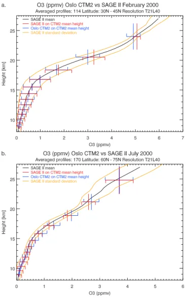
Recently the Oslo CTM2 (including stratospheric and tro-pospheric chemistry) has been improved by a new hetero-geneous and microphysics scheme which is described by Søvde et al. (2007)1. It is found to reproduce ozone deple-tion events like the Ozone Hole and miniholes. An exten-sive evaluation of the Oslo CTM2 is also given by Søvde et al. (2007)1, evaluating the model against aircraft, sonde and satellite measurements. Aircraft (Mozaic) flight measure-ments of ozone are found to be well reproduced on hourly ba-sis for both T42 and T21 horizontal resolution, although T42 performed best. Furthermore, sonde and satellite measure-ments of ozone were reproduced well. The conditions where T21 performed significantly poorer than T42 was in Ozone Hole conditions where the averaging of polar grids cause too much diffusion across the polar vortex. Comparisons of the Oslo CTM2 with a number of vertical profiles from SAGE II for a standard 2000 run are shown for two latitude intervals (30 N–45 N and 60 N–75 N, respectively) in Figs. 1a and b. The modelled profiles are taken at the same hour and location (grid box value) as the measurements, showing that ozone is well reproduced in the UTLS. Due to the intermediate life-time of ozone in the UTLS region, accurate transport as well as chemistry is needed to reproduce measurements. The eval-uation of the Oslo CTM2 presented here shows that the Oslo CTM2 performs well.
1Søvde, O. A., Gauss, M., Smyshlyaev, S., and Isaksen, I. S. A.:
The cold Arctic winter stratosphere of 2004/2005 – a Global Chemi-cal Transport Model study, J. Geophys. Res., to be submitted, 2007.
Fig. 1. Evaluation of Oslo CTM2 against SAGE II between 8 and
28 km altitude. Monthly mean ozone for (a) February 2000 between 30 N and 45 N, and (b) July 2000 between 60 N and 75 N. The aver-age SAGE II ozone profile is given as the black line, and its standard deviations as the orange lines. The blue vertical lines are the Oslo CTM2 averages on each model level, and red is SAGE II averaged on the same model levels. Standard deviations are given as horizon-tal bars for each model level.
A parameter closely connected to transport and the Brewer-Dobson circulation is the age of stratospheric air (Hall and Plumb, 1994). Monge-Sanz et al. (2007) used the ECMWF operational (4D-var) data extending to 0.1 hPa. The age of air for was improved when forecasts on 3 h time res-olution was used. For the 40-layer version of meteorological data applied here, we calculated the mean age of air from the age spectrum (according to Hall et al. (1999)), using the applied 2000 meteorology perpetually for 20 years, giving a zonal mean age maximum of 5.7 years at the top of the model domain (Fig. 2). The values at 20 km vary from 4.2 years at
Fig. 2. Mean age of air for the Oslo CTM2 in T21 horizontal
reso-lution, calculated using year 2000 meteorology. See text for details.
the South Pole to 1.3 in the tropics and 3.8 years at the North Pole, corresponding closely to the observed values shown by Monge-Sanz et al. (2007). Ideally the meteorological data should cover the whole stratosphere to assess the age of air. However, based on the calculated age presented here com-bined with the ability of reproducing measurements, we are confident that transport processes are well represented.
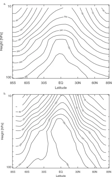
Our confidence is confirmed by looking at the longlived species, and in Fig. 3 the modelled annual mean N2O is
com-pared to the UARS Reference Atmosphere Project climatol-ogy available from their web-site http://code916.gsfc.nasa. gov/. The main structure of the atmospheric circulation with upwelling in the tropics and subsidence at high latitudes is covered, as well as the N2O levels. Modelled gradients at low
to mid latitudes above 20 km are somewhat underestimated, which is partly due to the coarse model vertical resolution at the highest altitudes, but also due to the upper boundary values, which are too low at low latitudes and too high at high latitudes. In this way reproduction of steep gradients observed is hindered by the boundary conditions, which pre-vents downward transport of low N2O at high latitudes. All
in all, the model is reproducing measurements well.
2.1.1 Emission set-up
The natural and industrial emissions are taken from the EU project POET (Precursors of Ozone and their Effects in the Troposphere) (POET report, 1999). The model is set up to simulate the year 2050 according to the SCENIC project (Rogers, 2005), where the industrial emissions of NOx, CO
and volatile organic compounds (VOC) are scaled up from the year 2000 by 2.2, 1.53 and 1.55, respectively. As the ini-tial chemical conditions, we use a steady-state atmospheric composition from a calculation of a previous 2050 study,
Fig. 3. Annual mean N2O from (a) the Oslo CTM2 and (b) the
UARS Reference Atmosphere Project climatology.
with the same boundary conditions. The boundary condi-tions in both studies were based on World Meteorological Organization (2003) for longlived species (e.g. CFCs), and methane and N2O were set to 2549 ppbv and 372 ppbv,
re-spectively, at the surface. Also emissions of stratospheric species were set to 2050 level, as were the model upper boundary conditions for all species (taken from the Oslo 2-D model (Stordal et al., 1985)). Otherwise, natural emissions are set to the level of year 2000. In the Oslo CTM2, tro-pospheric water vapor is retrieved from the meteorological data, while stratospheric water vapor is calculated assuming that the H2 content in water vapor, methane and hydrogen
gas is constant (Hsum=H2O+2CH4+H2), where only CH4is
transported. Hsum is set to 8.598 ppmv excluding aircraft
emissions of H2O. However, the H2O emitted from aircraft is
transported as a separate species, which is superposed on this calculated value of H2O. If PSC2 is formed, the solid H2O
is calculated and removed from the gas phase, and we keep track of the sedimented amount of solid H2O, thereby taking
dehydration into account.
Starting from the initial conditions (the previous 2050 study), a spin-up of 7 years without aircraft emissions was performed, followed by additional six-year runs including each of the aircraft emission scenarios, where results from the last year of the simulations are presented here. The air-craft emission inventories studied in this work are listed in Table 1, and are given in 1x1 degrees horizontal resolution and 305 m vertical resolution. These data are interpolated into the Oslo CTM2 grid each model time step. Due to the relatively coarse horizontal model resolution, a plume model is applied to the aircraft emissions (Kraabøl et al., 1999) to include the effects of in-plume chemistry, changing the NOx
partitioning of the emissions. In this way the plume pro-cessed emissions can be emitted into the model grid.
Based on a predicted increase in non-commercial as well as commercial aircraft traffic, emissions from the most likely mixed fleet is given in MIX, assuming 501 supersonic air-craft and 114.1 million supersonic passengers per year and a supersonic aircraft cruise speed of 2.0 Mach. Aircraft emis-sions in this study include NOx and H2O, omitting other
products of fuel combustion such as CO2, CO, different
hy-drocarbons and sulfur oxides; although CO2is an important
greenhouse gas, the lifetime is too long to distinguish the aircraft effect from other sources, and increases of the other combustion products are low compared to the background concentrations, hence they are expected to have a small at-mospheric impact (Fabian and K¨archer, 1997). The aircraft emissions comprise commercial subsonic, commercial su-personic, general aviation and military fleet, and the respec-tive emissions of NOxand H2O are listed in Table 2. H2O
emissions are calculated as 1.25 of fuel burned.
NOx in the troposphere produces ozone in the presence
of peroxy radicals and sunlight, while in the stratosphere it causes ozone depletion through the catalytic NOxcycle. H2O
is an important source of the OH radical (H2O+O1D→2OH),
which contributes to ozone loss. In this study we focus on the total atmospheric impact of NOx and H2O emissions. Due
to the high background concentration of H2O in the
tropo-sphere, the effects of H2O emissions in the troposphere are
negligible. However, in the stratosphere H2O is very low,
and therefore aircraft emissions have a larger effect on the OH formation.
Scenario AERO is similar to MIX, except that aircraft aerosol emissions are included. Aerosols offer surfaces for heterogeneous chemistry, which is important for NOx
chem-istry. The surface area density (SAD) of these aerosols was included in the model as a transported tracer with SAD-emissions calculated according to Danilin et al. (1998),
SAD = 3µfρaξEI(S)µH2SO4
rρswH2SO4µS
Table 1. The aircraft scenarios used in this study.
NOx H2O Aerosol
Scenario Fleet emissions emissions emissions noAC No aircraft no no no
MIX Sub- and supersonic (mixed) fleet See Table 2 no AERO MIX with aerosol emissions as MIX as MIX yes noH2O MIX without H2O emissions as MIX no no
noBACK MIX without background aerosols as MIX as MIX no
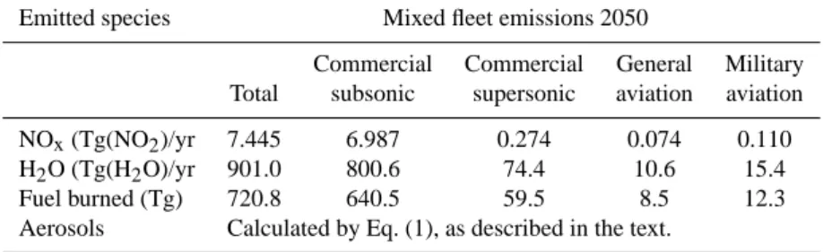
Table 2. The aircraft scenario emissions of the mixed fleet taken from Marizy et al. (2007)??.
Emitted species Mixed fleet emissions 2050
Commercial Commercial General Military Total subsonic supersonic aviation aviation NOx(Tg(NO2)/yr 7.445 6.987 0.274 0.074 0.110
H2O (Tg(H2O)/yr 901.0 800.6 74.4 10.6 15.4
Fuel burned (Tg) 720.8 640.5 59.5 8.5 12.3 Aerosols Calculated by Eq. (1), as described in the text.
where ρs=1.5 gcm−3is the density of sulfur, ρais the den-sity of air, wH2SO4=50% is the weight percent of sulfuric
acid and µS and µH2SO4 are the molecular weights of
sul-fur and sulsul-furic acid, respectively. The particle radius is assumed to be r=10 nm, and the emission index of sulfur is EI(S)=4×10⁻⁴. The fuel mixing ratio (µ
f) is calculated from the MIX NOxemissions applying the EI(NOx) for
su-personic aircraft (4.6 g/kg). Even though subsonic aircraft have a higher emission index for NOxand may result in a too
low SAD value for the subsonic flight levels, the application of the chosen emission index is justified by the uncertainty of EI(S) and the conversion factor (ξ =0.05) of sulfur to sul-fate, and the fact that the particles will be most important in the stratosphere. To simulate washout of emitted species, a method suggested by Danilin et al. (1998) is used, where emitted gases and aerosols are removed with e-folding time of 5 days below 400 hPa. In the top model layer, an e-folding time of 1 year is applied to simulate transport and mixing upwards. In this study, sedimentation of aircraft aerosols is not considered, but will be discussed in Sect. 5. Air-craft aerosol emissions are superimposed on the Oslo CTM2 background aerosols, which are taken from a monthly zonal mean SAD climatology derived from various satellite mea-surements, primarily SAGE II according to Thomason et al. (1997), and data for the year 1999 is applied. A sensitiv-ity study of the MIX scenario without background aerosols (noBACK) is also carried out.
3 Impact of emissions from a mixed fleet
Subsonic and supersonic aircraft cruise at different altitudes. The subsonic fleet is larger than the supersonic fleet, giv-ing the largest contribution to aircraft NOxemissions. This
is clearly seen from Fig. 4, showing the annual zonal mean change in reactive nitrogen (NOy) with maximum increase at
11 km, and a secondary maximum at about 18 km. Clearly, the secondary maximum is due to supersonic aircraft, while the 11 km maximum is due to subsonic aircraft. The sea-sonal variation of the monthly zonal mean maximum due to subsonic aircraft ranges from 1.1 in September to 1.9 ppbv in May (Fig. 5). During winter and spring, a larger fraction is emitted into the stratosphere than during summer months due to a lower tropopause, increasing the impact of subsonic aircraft. The higher tropopause in summer is accompanied by relatively strong convection, mixing and washout at mid-latitudes, leading to a reduction in the NOyincreases in the
mid-latitude troposphere. This causes the maximum impact of aircraft emissions to shift northward (Kraabøl et al., 2002). A similar latitude shift of the maximum value is reported by Gauss et al. (2003a).
Although the contribution of supersonic aircraft to the zonal mean change is much smaller than for subsonic air-craft, the maximum NOychanges due to supersonic aircraft
are locally comparable with subsonic aircraft emissions, es-pecially in the summer months. Supersonic flights are con-fined mostly to the North Atlantic corridor, and this small zonal extent results in the slightly lower zonal mean maxi-mum shown in Fig. 4.
Fig. 4. Effect of mixed fleet aircraft emissions on NOy, annual
zonal mean (MIX minus noAC). Max: 1.35 ppbv.
Fig. 5. Latitude and magnitude variation of the monthly mean
max-imum effect of aircraft emissions on NOy(MIX minus noAC): 1.1
to 1.9 ppbv.
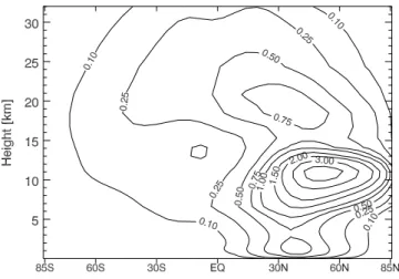
Aircraft emissions of H2O contribute to an annual zonal
mean increase of up to 624 ppbv above the background H2O
(Fig. 6), ranging from 609 to 833 ppbv in the monthly mean. The maximum change in monthly zonal mean H2O due to
aircraft is mainly located at 11 km altitude, and is largest dur-ing summer when the maximum shifts to higher altitudes. As seen before, this shift is caused by higher tropopause lev-els extending transport and washout processes to higher alti-tudes.
The annual zonal mean effect of aircraft emissions (NOx
and H2O) on ozone is given in Fig. 7, showing a
maxi-mum of 10 ppbv at 10 km and a minimaxi-mum of −39 ppbv at 24 km. From month to month, these values vary from 7.2 to 18.4 ppbv (corresponding to a change of 5.5 to 8.9%) and
Fig. 6. Effect of aircraft emissions on H2O, annual zonal mean
(MIX minus noAC). Max: 629.69 ppbv.
from −48.8 to −31.4 ppbv (−1.8 to −0.8%), respectively (Fig. 8). The maximum variation largely follows the vari-ation of the NOymaximum, but at an altitude of 9–10 km.
This means that the maximum ozone production is located at a lower altitude than the maximum of emissions. Unlike NOyand NOx, the maximum ozone increase is shifted
north-wards for a longer time period in spring and summer, partly due to a higher tropopause and more washout processes at mid-latitudes. Also important for this shift is the increased amount of sunlight at high latitudes during spring and sum-mer, causing more ozone production even for moderate NOx
increases.
NOx contributes to ozone production in the presence of
sunlight and peroxy radicals. At some altitude (the turn-over point), the amount of these radicals is too low for ozone pro-duction, and the catalytic NOx cycle takes over, reducing
ozone. The zero line of Fig. 7 does not represent the turn-over point, since transport processes also affect this figure: Downward transport of ozone depleted air will lower the al-titude of the zero line. H2O emissions, however, contribute to
ozone destruction at all altitudes through the OH chemistry. Looking at Fig. 8, the monthly variation of maximum ozone depletion due to aircraft resembles the variation of maximum production. The maximum depletion is located at about 30– 40 N, around 24 km, except during summer months, when a shifting northwards is seen, accompanied by a lowering of the maximum depletion to about 20 km altitude. This shift is due to stratospheric transport processes and more sunlight at higher latitudes. Being located above the NOx and NOy
maxima, the maximum ozone depletion is caused by upward transport of NOxand H2O, followed by more effective
deple-tion at higher altitudes. Most of this ozone depledeple-tion is due to supersonic aircraft; only a small fraction originates from the upward transport of subsonic aircraft emissions. Mixing
Fig. 7. Effect of aircraft emissions on O3, annual zonal mean (MIX minus noAC). Min: −39.24 ppbv, max: 9.96 ppbv.
Fig. 8. Magnitude and latitude variation of the monthly zonal mean
maximum/minimum effect of aircraft emissions on O3(MIX minus
noAC), maximum ranging from 7.2 to 18.4 ppbv (due to subsonic aircraft) and minimum from −48.8 to −31.4 ppbv (due to super-sonic aircraft).
of tropospheric (ozone increased) and stratospheric (depleted ozone) air in a mixed fleet scenario will therefore lower the tropospheric ozone increase due to subsonic aircraft.
Inter-hemispheric transport of stratospheric aircraft emis-sions is clearly seen in Figs. 4 and 6, in contrast to trans-port of subsonic aircraft emissions at lower altitudes, which is very limited (not shown). The high altitude transport will affect ozone in the Southern Hemisphere although emissions occur in the Northern Hemisphere.
When affecting ozone, aircraft emissions may also alter the total ozone column. The changes in daily zonal averages of the total ozone columns for the last two simulated years
Fig. 9. Changes in the daily zonal mean total ozone column
[Dob-son Units] due to aircraft emissions (MIX minus noAC) for the last two years of simulation, ranging from −1.56 DU to 1.65 DU.
are shown in Fig. 9, ranging from −1.56 DU to 1.65 DU. The increase in the total column is located in the area of highest flight density. At higher latitudes, however, the su-personic aircraft contribute more to ozone loss, showing a net decrease in the total column, except during spring and summer months where the ozone production maximum is shifted northwards, overriding the ozone loss at higher al-titudes. The ozone decrease in the Southern Hemisphere is mainly due to cross-hemispheric transport of emissions from supersonic aircraft, and to some extent transport of ozone de-pleted air. From August to October, there is also a decrease in total ozone in the tropical region. This is because the tro-pospheric ozone production due to aircraft emissions is small due to a high tropopause and increased washout of NOy
dur-ing these months, causdur-ing the stratospheric depletion to dom-inate.
A sensitivity study omitting aircraft emissions of H2O
(scenario noH2O) reveals that ozone changes due to aircraft emissions are mainly caused by NOx. This is carried out
looking at the MIX – noH2O difference. Emissions of H2O
give maximum ozone losses ranging from 6.7 to 11.4 ppbv in the monthly zonal mean (not shown). The maximum effect of H2O on ozone is generally located at 25–30 N and 24 km
height with values ranging from 6 to 7 ppbv. However, the largest decrease in ozone is found in October–November due to PSC chemistry taking place at about 18 km at the South Pole. The ozone reduction due to aircraft emissions of H2O
is most prominent in the stratosphere, although there is some ozone reduction caused by H2O in the troposphere. At the
highest latitudes around 24 km altitude and during summer, H2O emissions slightly enhance heterogeneous chemistry on
background aerosols, reducing NOx and thereby increasing
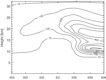
Fig. 10. Annual zonal mean of aircraft aerosol surface area density
from the mixed fleet. Max: 4.7 µm2cm−3.
4 Impact of aerosol emissions from a mixed fleet
Heterogeneous reactions may take place on sulfate aerosols converting NOxinto HNO3– reactions being most effective
at low temperatures. Depending on the altitude of this con-version, the resulting reductions of NOx will either reduce
the production of ozone in the troposphere and lowermost stratosphere, or reduce the loss at higher altitudes. However, the formation of PSCs and chlorine activation may be en-hanced by a reduction of NOx.
Calculating the aircraft aerosol SAD emissions based on the method of Danilin et al. (1998), we find an annual zonal average SAD maximum of 4.7 µm2/cm3(Fig. 10), the monthly zonal mean maximum varying steadily through the year (Fig. 11), ranging from 3.8 µm2/cm3in September to 6.2 µm2/cm3in May. As for NOyemissions, the largest
val-ues are found in the Northern Hemispheric winter and spring at about 47 N and 11 km height, also shifting slightly to the north during summer and autumn because of the meteoro-logical conditions. Although the maximum value decreases during summer conditions, the surface area density values in the stratosphere increase due to upward transport. The tropospheric reduction of NOx due to aerosol emissions is
largest in spring, while the stratospheric reduction is largest in autumn. Hence, the largest reduction of ozone production due to aerosol emissions from aircraft occurs during spring, while the largest reduction of ozone loss at higher altitudes takes place in autumn.
The heterogeneous conversion of NOxto HNO3will also
occur on background aerosols, similarly affecting the pro-duction and loss of ozone. In Fig. 12 we see the annual zonal mean effect of aircraft aerosol emissions on ozone (AERO – MIX), superimposed on the effect of background aerosols (MIX – noBACK), for latitudes between 30 and 60 degrees in (a) the Northern and (b) Southern Hemisphere. Most
promi-Fig. 11. Variation of the magnitude and latitude of the monthly
zonal mean maximum of aircraft aerosol surface area density.
Fig. 12. Annual zonal mean effect of background aerosol on O3
(cross-hatched) and the contribution from aircraft aerosol emissions (hatched). (a): 30 N–60 N, (b): 60 S–30 S (given in ppbv).
nent is the increase in ozone between 18 and 30 km due to ozone loss reduction, where the effect of aircraft aerosols is comparable with the background aerosols. For altitudes be-tween 12 and 20 km aircraft aerosols contribute to an ozone reduction through reduced production and a slight increase in ozone loss due to more PSCs or supercooled ternary solu-tions (STS).
The amount of PSCs is dependent on HNO3and H2SO4,
where the latter is calculated from the amount of background aerosols available (described by Søvde et al., 20071). Thus an increase in HNO3and H2SO4due to aircraft aerosol
Fig. 13. Annual zonal mean effect of a mixed fleet with aerosol
emissions on O3(AERO minus noAC), given in ppbv.
increase in ozone loss. Also, a reduction in NOxwill result
in more active chlorine available for depleting ozone. These effects are apparent at altitudes between 12 and 20 km.
The maximum increase of ozone for a mixed fleet includ-ing aerosol emissions (Fig. 12), has a larger magnitude than the maximum decrease due to NOxand H2O emissions only
(Fig. 7). Aircraft aerosols give a reduction of NOxthrough
heterogeneous reactions, reducing the loss of ozone due to the NOx cycle. The increase in aerosol SAD also
inten-sify the heterogeneous conversions, lowering the concentra-tion of HCl and thus the heterogeneous loss of ClONO2. In
this way more NOxis bound up in ClONO2, while also the
ClO is increased, since less NO2 is available for forming
ClONO2. The same applies for BrO/BrONO2. Both NOx
and ClO are responsible for ozone loss, so by looking at the effect on ozone (AERO – noAC, Fig. 13) we see that above 18−20 km the NOxcycle is more important for ozone than
the ClO – giving an increase of ozone due to reduced NOx.
From 18−20 km and down to about 11−12 km (lower at the Southern Hemisphere), the turn-over point where NOxstarts
to produce ozone will be reached. However, in this region enhanced ClO and BrO increase the ozone loss in addition to the reduced ozone production due to lower NOx. Below
11−12 km the NOx reduction due to aerosols is not large
enough to overcome the aircraft emissions of NOx,
result-ing in increased ozone production there (Fig. 13). Therefore, a mixed fleet with aerosol emissions results in an increase in the daily zonal mean total column at most latitudes (Fig. 14; AERO minus noAC). At the lowermost latitudes through the year, and at the highest latitudes during summer, the reduced ozone production and enhanced loss due to ClO cause a de-crease in ozone. The ozone column reduction at high lati-tudes during spring is due to increased heterogeneous chem-istry on PSCs and therefore increased ozone loss due to ClO.
Fig. 14. Changes in the daily zonal mean total ozone column [Dobson Units] due to the mixed fleet aircraft emissions including aerosol emissions (AERO minus noAC), for the last two years of simulations, ranging from −1.67 DU to 3.34 DU.
Separating the effect of aircraft aerosols, by comparing the AERO scenario to the mixed fleet scenario (MIX), aircraft aerosols reduces the total ozone column in spring, and in-crease it in autumn (Fig. 15). Again, the dein-crease is due to reduced ozone production below the turn-over point (about 20 km), combined with increased ozone loss by ClO and due to heterogeneous reactions on PSCs/STS. The increase is due to ozone loss decrease at higher altitudes (Fig. 16). The decrease in ozone column near the North Pole during May through June is due to more ozone loss below 20 km (due to ClO increase and reduced ozone production) than the ozone loss is decreased above 20 km (due to NOx). Aerosols
are also transported into the Southern Hemisphere, readily reducing NOx there as well, giving similar results,
how-ever smaller in magnitude. The cross-hemispheric transport is most effective above 18 km, mainly resulting in reduced ozone loss. However, ClO is also increased here, to some ex-tent enhancing the ozone loss below 18 km. The ozone loss is also increased in spring when heterogeneous chemistry on PSCs/STS is enhanced, increasing the Ozone Hole depth.
Stratospheric H2O increases slightly due to the presence
of aircraft aerosols (not shown), with an annual zonal mean maximum increase after six years of 7.3 ppbv. This is due to heterogeneous reactions on the aerosols, leading to H2O
production from methane: Because the stratospheric H2O in
the model is calculated assuming constant total hydrogen, a decrease in methane will increase the amount of H2O.
Fig. 15. Changes in the daily zonal mean total ozone column
[Dob-son Units] due to the mixed fleet aerosol emissions (AERO minus MIX), for the last two years of simulations, ranging from −0.73 DU to 4.51 DU.
5 Discussion and conclusions
We have shown that aerosol emissions in a projected future (2050) “mixed fleet” of subsonic and supersonic aircraft are likely to increase stratospheric ozone due to a lowered loss to NOx, leading to an increase in the total ozone column.
Without aerosol emissions, subsonic aircraft are found to in-crease tropospheric ozone and lower stratospheric ozone in agreement with previous studies, although with a larger im-pact (7 to 18 ppbv ozone increase in the monthly zonal mean) compared to previous studies of present impact (3 to 8 ppbv; Gauss et al., 2006a). Similarly, supersonic aircraft are es-timated to give ozone depletion in the stratosphere (31 to 49 ppbv as monthly zonal mean). A mixed fleet will there-fore reduce the total ozone column compared to a subsonic fleet. Reduced stratospheric ozone in the Southern Hemi-sphere is a result of cross hemispheric transport of ozone depleted air. At northern high latitudes, aircraft emissions cause an increase in the total ozone column in spring and early summer – when transport processes and the amount of sunlight increase the ozone production – and a decrease in autumn.
The maximum contribution of H2O emissions from a
mixed fleet to stratospheric ozone depletion ranges from 6.7 to 11.4 ppbv in the monthly zonal mean. The largest effect is found to occur through heterogeneous chemistry in October and November.
When aircraft aerosol emissions are introduced, NOx
lev-els are reduced due to heterogeneous chemistry, while ClO levels increase. This results in enhanced ozone loss in the 11−20 km region. To some extent aircraft aerosols will also
Fig. 16. Annual zonal mean effect of aircraft aerosol emissions on
O3(AERO minus MIX), given in ppbv.
reduce tropospheric NOx and therefore ozone production,
contributing to a reduction of the total ozone column. The heterogeneous chemistry and the lowered production con-tributes to a reduction in the total ozone column, whereas the stratospheric NOxreduction contribute to an ozone column
increase.
An increase in the surface area density of aerosols con-verts more NOxto HNO3and the reduction of NOxactivates
more chlorine, and increase ozone loss due to PSCs. Back-ground aerosols at kept at the low 1999 level. Increases in the background aerosols increase, e.g. due to volcanic erup-tions, will affect NOxand the ozone loss. Likewise, adopting
the 2000 meteorology as a reference for this study to ensure stable steady-state results, could have an impact on the cal-culated perturbations. The year 2000 has been reported to exhibit a cold bias near the tropopause (Randel et al., 2004). In a too cold UTLS region the heterogeneous conversions would be overestimated which would lead to a smaller O3
-loss due to NOxand larger loss due to halogens. In respect
to this, the 2000 UTLS could be more similar to year 2050 conditions with increased CO2levels. Assessing the impact
of meteorology on the chemical perturbations in the UTLS region is being done in another study.
Although T21 reproduces the main features of measure-ments, it is a rather coarse horizontal resolution. We find it sufficient for this study, combined with the applied aircraft plume model. Increasing the resolution to T42 will be done in the future, as well as increasing the vertical resolution to cover the whole stratosphere.
It should be noted that we have assumed no sedimentation of aircraft aerosols. If included, the effect of the calculated aerosol surface area density would probably be somewhat reduced, with the result that the ozone reduction due to lowered NOxand increased ClO would be smaller, possibly
resulting in a decrease in the total ozone column. Neverthe-less, aircraft aerosol emissions seem to be an important part of the stratospheric aircraft emissions.
Edited by: W. Collins
References
Airbus: Global Market Forecast 2004–2023, Published at the Air-bus S.A.S. website, http://www.airAir-bus.com/, 2004.
Berntsen, T. and Isaksen, I. S. A.: A global 3-D chemical transport model for the troposphere, 1, Model description and CO and Ozone results, J. Geophys. Res., 102, 21 239–21 280, doi:10.1029/97JD01140, 1997.
Braathen, G., Arlander, B., Dahlback, A., Edvardsen, K., Engelsen, O., Fløisand, I., Gauss, M., Hansen, G., Hoppe, U.-P., Høiskar, B. A. K., Isaksen, I., Kjeldstad, B., Kylling, A., Orsolini, Y., Rognerud, B., Stordal, F., Sundet, J., Thorseth, T. M., and Tørnkvist, K. K.: COSUV, third annual report, Norwegian insti-tute for air research (NILU), http://www.nilu.no/projects/cozuv/, 2003.
Brasseur, G. P., Cox, R. A., Hauglustaine, D., Isaksen, I., Lelieveld, J., Lister, D. H., Sausen, R., Schumann, U., Wahner, A., and Wiesen, P.: European scientific assessment of the atmospheric effects of aircraft emissions, Atmos. Environ., 32, 2329–2418, doi:10.1016/S1352-2310(97)00486-X, 1998.
Brunner, D., Staehelin, J., Rogers, H. L., K¨ohler, M. O., Pyle, J. A., Hauglustaine, D., Jourdain, L., Berntsen, T. K., Gauss, M., Isak-sen, I. S. A., Meijer, E., van Velthoven, P., Pitari, G., Mancini, E., Grewe, V., and Sausen, R.: An evaluation of the performance of chemistry transport models by comparison with research aircraft observations. Part 1: Concepts and overall model performance, Atmos. Chem. Phys., 3, 1609–1631, 2003,
http://www.atmos-chem-phys.net/3/1609/2003/.
Brunner, D., Staehelin, J., Rogers, H. L., K¨ohler, M. O., Pyle, J. A., Hauglustaine, D. A., Jourdain, L., Berntsen, T. K., Gauss, M., Isaksen, I. S. A., Meijer, E., van Velthoven, P., Pitari, G., Mancini, E., Grewe, V., and Sausen, R.: An evaluation of the performance of chemistry transport models – Part 2: Detailed comparison with two selected campaigns, Atmos. Chem. Phys., 5, 107–129, 2005,
http://www.atmos-chem-phys.net/5/107/2005/.
Dameris, M., Grewe, V., K¨ohler, I., Sausen, R., Brhl, C., Groo, J.-U., and Steil, B.: Impact of aircraft NOx emissions on tropospheric and stratospheric ozone. part II: 3-D model re-sults, Atmos. Environ., 32, 3185–3199, doi:10.1016/S1352-2310(97)00505-0, 1998.
Danilin, M. Y., Fahey, D. W., Schumann, U., Prather, M. J., Pen-ner, J. E., Ko, M. K. W., Weisenstein, D. K., Jackman, C. H., Pitari, G., K¨ohler, I., Sausen, R., Weaver, C. J., Douglass, A. R., Connell, P. S., Kinnison, D. E., Dentener, F. J., Flem-ing, E. L., Berntsen, T. K., Isaksen, I. S. A., Haywood, J. M., and K¨archer, B.: Aviation fuel tracer simulation: Model inter-comparison and implications, Geophys. Res. Lett., 25, 3947, doi:10.1029/1998GL900058, 1998.
Eskes, H. E. A.: The EU project GOA – GOME Assimilated and Validated Ozone NO2 Fields for Scientific Users and for Model
Validation, Project Final report, project Final Report, Contract No. EVK2-CT-2000-00062, 2003.
Fabian, P. and K¨archer, B.: The Impact of Aviation upon the At-mosphere, Physics and Chemistry of The Earth, 22, 503–598, doi:10.1016/S0079-1946(97)00181-X, 1997.
Gauss, M.: Impact of aircraft emissions and ozone changes in the 21st century: 3-D model studies, Ph.D. thesis, University of Oslo, Department of Geophysics, Section of Meteorology and Oceanography, PB. 1022 Blindern, 0315 Oslo, Norway, iSSN 1501-7710, No. 304, 2003.
Gauss, M., Isaksen, I. S. A., Lee, D., and Søvde, A.: Present and fu-ture impact of aircraft NOx emissions on the atmosphere – Trade-offs to reduce the impact, Institute report series, 123, department of Geosciences, University of Oslo, Oslo, Norway, 2003a. Gauss, M., Isaksen, I. S. A., Wong, S., and Wang, W. C.:
Impact of H2O emissions from cryoplanes and kerosene aircraft on the atmosphere, J. Geophys. Res., 108, 4304, doi:10.1029/2002JD002623, 2003b.
Gauss, M., Myhre, G., Pitari, G., Prather, M. J., Isaksen, I. S. A., Berntsen, T. K., Brasseur, G. P., Dentener, F. J., Derwent, R. G., Hauglustaine, D. A., Horowitz, L. W., Jacob, D. J., Johnson, M., Law, K. S., Mickley, L. J., M¨uller, J.-F., Plantevin, P.-H., Pyle, J. A., Rogers, H. L., Stevenson, D. S., Sundet, J. K., van Weele, M., and Wild, O.: Radiative forcing in the 21st century due to ozone changes in the troposphere and the lower stratosphere, J. Geophys. Res., 108, 4294, doi:10.1029/2002JD002624, 2003c. Gauss, M., Isaksen, I. S. A., Lee, D. S., and Søvde, O. A.: Impact of
aircraft NOx emissions on the atmosphere - tradeoffs to reduce the impact, Atmos. Chem. Phys., 6, 1529–1548, 2006a. Gauss, M., Myhre, G., Isaksen, I. S. A., Grewe, V., Pitari, G., Wild,
O., Collins, W. J., Dentener, F. J., Ellingsen, K., Gohar, L. K., Hauglustaine, D. A., Iachetti, D., Lamarque, J.-F., Mancini, E., Mickley, L. J., Prather, M. J., Pyle, J. A., Sanderson, M. G., Shine, K. P., Stevenson, D. S., Sudo, K., Szopa, S., and Zeng, G.: Radiative forcing since preindustrial times due to ozone change in the troposphere and the lower stratosphere, Atmos. Chem. Phys., 6, 575–599, 2006b.
Grewe, V., Dameris, M., Fichter, C., and Lee, D. S.: Im-pact of aircraft NOx emissions. Part 2: Effects of lowering the flight altitude, Meteorologische Zeitschrift, 11, 197–205, doi:10.1127/0941-2948/2002/0011-0197, 2002.
Grini, A., Myhre, G., Sundet, J. K., and Isaksen, I. S. A.: Mod-eling the annual cycle of sea salt in the global 3-D model Oslo CTM-2, J. Climate, 15, 1717–1730, doi:10.1175/1520-0442(2002)015¡1717:MTACOS>2.0.CO;2, 2002.
Hall, T. M. and Plumb, R. A.: Age as a diagnostic of stratospheric transport, J. Geophys. Res., 99, 1059–1070, doi:10.1029/93JD03192, 1994.
Hall, T. M., Waugh, D. W., Boering, K. A., and Plumb, R. A.: Evaluation of transport in stratospheric models, J. Geophys. Res., 104, 18 815–18 839, doi:10.1029/1999JD900226, 1999. Hesstvedt, E., Hov, O., and Isaksen, I. S. A.: Quasi steady-state
approximation in air pollution modelling: Comparison of two numerical schemes for oxidant prediction, Int. J. Chem. Kinetics, X, 971–994, 1978.
Hidalgo, H. and Crutzen, P. J.: The tropospheric and stratospheric composition perturbed by NOx emissions of high-altitude air-craft, J. Geophys. Res., 82, 5833–5866, 1977.
resolution air mass transformation model for short-range weather forecasting, Mon. Wea. Rev., 118, 1561–1575, 1990.
Isaksen, I. S. A.: The EU project TRADEOFF – Aircraft emissions: Contributions of various climate compounds to changes in com-position and radiative forcing – tradeoff to reduce atmospheric impact, Project Final report, 2003.
Isaksen, I. S. A., Rognerud, B., Stordal, F., Coffey, M. T., and Mankin, W. G.: Studies of Arctic stratospheric ozone in a 2-d model including some effects of zonal asymmetries, Geophys. Res. Lett., 17, 557–560, 1990.
Isaksen, I. S. A., Zerefos, C., Kourtidis, K., Meleti, C., Dalsøren, S. B., Sundet, J. K., Grini, A., Zanis, P., and Balis, D.: Tro-pospheric ozone changes at unpolluted and semipolluted regions induced by stratospheric ozone changes, J. Geophys. Res., 110, D02 302, doi:10.1029/2004JD004618, 2005.
Johnson, C., Henshaw, J., and McInnes, G.: Impact of aircraft and surface emissions of nitrogen oxides on tropospheric ozone and global warming, Nature, 355, 69–71, doi:10.1038/355069a0, 1992.
Johnston, H. S.: Reduction of stratospheric ozone by nitrogen oxide catalysts from supersonic transport exhaust, Science, 173, 517– 522, 1971.
Kawa, S. R., Anderson, J. G., Baughcum, S. L., Brock, C. A., Brune, W. H., Cohen, R. C., Kinnison, D. E., Newman, P. A., Rodriguez, J. M., Stolarski, R. S., Waugh, D., and Wofsy, S. C.: Assessment of the Effects of High-Speed Aircraft in the Strato-sphere 1998, Tech. rep., NASA, nASA TP-1999-209237, 1998. Kraabøl, A. G., Stordal, F., Konopka, P., and Knudsen, S.: The
NILU aircraft plume model: A technical description, Tech. Rep. TR 4/99, Norwegian Institute for Air Research, 1999.
Kraabøl, A. G., Berntsen, T. K., Sundet, J. K., and Stordal, F.: Impacts of NOx emissions from subsonic aircraft in a global three-dimensional chemistry transport model in-cluding plume processes, J. Geophys. Res., 107, 4655, doi:10.1029/2001JD001019, 2002.
Monge-Sanz, B. M., Chipperfield, M. P., Simmons, A. J., and Up-pala, S. M.: Mean age of air and transport in a CTM: Comparison of different ECMWF analyses, Geophys. Res. Lett., 34, L04801, doi:10.1029/2006GL028515, 2007.
POET report: Present and future emissions of atmospheric com-pounds, EU report EV K2-1999-00011, web site: http://nadir. nilu.no/poet/, 1999.
Prather, M. J.: Numerical advection by conservation of second-order moments, J. Geophys. Res., 91, 6671–6681, 1986. Randel, W. J., Wu, F., Oltmans, S. J., Rosenlof, K., and
Nedoluha, G. E.: Interannual Changes of Stratospheric Wa-ter Vapor and Correlations with Tropical Tropopause Tem-peratures, J. Atmos. Sci., 61, 2133–2148, doi:10.1175/1520-0469(2004)061<2133:ICOSWV>2.0.CO;2, 2004.
Rogers, H. L.: SCENIC project: Scenario of aircraft Emissions and Impact studies on Chemistry and climate: Final Report, eU Project EVK2-2001-00103, 2005.
Rummukainen, M., Isaksen, I. S. A., Rognerud, B., and Stordal, F.: A global model tool for three-dimensional mul-tiyear stratospheric chemistry simulations: Model descrip-tion and first results, J. Geophys. Res., 104, 26 437–26 456, doi:10.1029/1999JD900407, 1999.
Schumann, U.: The impact of nitrogen oxides emissions from aircraft upon the atmosphere at flight altitudes – results from the aeronox project, Atmos. Environ., 31, 1723–1733, doi:10.1016/S1352-2310(96)00326-3, 1997.
Stolarski, R. S., Baughcum, S. L., Brune, W. H., Douglass, A. R., Fahey, D. W., Friedl, R. R., Liu, S. C., Plumb, R. A., Poole, L. R., and Wesoky, H. L.: The 1995 scientific assessment of the atmospheric effects of stratospheric aircraft, Tech. rep., NASA, nASA Technical Report, NASA-RP-1381, 1995.
Stordal, F., Isaksen, I. S. A., and Horntvedt, K.: A diabatic circu-lation two-dimensional model with photochemistry: Simucircu-lations of ozone and long-lived tracers with surface sources, J. Geophys. Res., 90, 5757–5776, 1985.
Thomason, L. W., Poole, L. R., and Deshler, T.: A global climatology of stratospheric aerosol surface area density de-duced from Stratospheric Aerosol and Gas Experiment II mea-surements: 1984-1994, J. Geophys. Res., 102, 8967–8976, doi:10.1029/96JD02962, 1997.
Tiedke, M.: A Comprehensive Mass Flux Scheme for Cumulus Pa-rameterisation on Large Scale Models, Mon. Wea. Rev., 117, 1779–1800, 1989.
World Meteorological Organization: Scientific assessment of ozone depletion: 2002., World Meteorological Organization: Global ozone research and monitoring project – Report 47, 498 pp, Geneva, Switzerland, 2003.