Anomalous Eurasian snow extent and the wintertime AO

(1)

Anomalous Eurasian Snow Extent and the Wintertime AO

by

Elizabeth Whitin Lundgren

B.S., Environmental Engineering Science B.S., Physics

Massachusetts Institute of Technology (2007)

Submitted to the Department of Civil and Environmental Engineering in partial Fulfillment of the Requirements for the Degree of

Master of Science

in Civil and Environmental Engineering at the

Massachusetts Institute of Technology June 2009

Signature of Author . . . . Department of Civil and Environmental Engineering

May 7, 2009 Certified by . . . .

Dara Entekhabi Bacardi and Stockholm Water Foundations Professor Thesis Supervisor Accepted by . . .

(2)

(3)

Anomalous Eurasian Snow Extent and the Wintertime AO

by

Elizabeth Whitin Lundgren

B.S., Environmental Engineering Science B.S., Physics

Massachusetts Institute of Technology (2007)

Submitted to the Department of Civil and Environmental Engineering in partial Fulfillment of the Requirements for the Degree of

Master of Science

in Civil and Environmental Engineering

Abstract

The winter mode of the Arctic Oscillation (AO) is the dominating influence on extratropical winter climate variability in the Northern Hemisphere (NH) . The phase of the Arctic Oscillation is characterized by trends in temperature, precipitation, air pressure, and storm tracks over the North Atlantic region, and affects northeastern North America, Europe, and parts of the Mediterranean. While predictability of the AO phase would benefit socio-economic sectors in these densely populated regions by enabling greater foreknowledge of energy demands, precipitation intensity, and storm frequency, it is currently not particularly skillful. Previous studies have demonstrated a link between autumn snow over Eurasia and the AO mode and have proposed a dynamical pathway describing the mechanism that links them.

The goal of this thesis is to present new evidence of a significant relationship between anomalous snow cover and the winter AO phase. Observational evidence of a significant link between extremely high (low) October snow extent anomalies over Eurasia and the negative (positive) AO winter phase is presented. Significant positive (negative) vertical wave activity flux (WAF) anomalies in the stratosphere during December and January are shown to occur following autumns with significantly high (low) snow extent, supporting the dynamical pathway proposed in previous studies. It is concluded that a significant mean snow extent anomaly over Eurasia in October could serve as a predictor for the AO phase of the following winter.

Thesis Supervisor: Dara Entekhabi

(4)

(5)

Dedicated to my mother,

Nancy Whitin Truslow Lundgren

Acknowledgments

Research for this thesis has been made possible by support from the Linden Earth System Initiative Fellowship and the National Science Foundation Grant ATM-0443451. ECMWF ERA-40 data used in this project was provided by the European Centre for Medium-range Weather Forecasting data server.

I am fortunate to have many wonderful people in my life who have nurtured and encouraged me throughout my graduate years at MIT. The professional and personal support I have received has been integral to my success and I am very grateful. I would like to give special thanks to my advisor, Dara Entekhabi, for guiding me in my scientific endeavors over the past two years. His excitement and encouragement proved always to bolster my morale and lend renewed energy to my work.

Professional support in my research has also been provided by Judah Cohen who has generously met with me multiple times to discuss my work. I greatly value the

comments and advice he has offered and thank him for his time and feedback. I owe tremendous gratitude to my father, Richard Lundgren, for always encouraging me to do whatever I want in life and always supporting me along the way. I also thank: Kristen Burrall for serving as a great peer throughout so many classes; Rhyland Gillespie for being a fabulous and fun partner every Friday night; and Julie Parker for being a great friend.

I would be remiss in not acknowledging Lindgren Library as a strong support for me throughout my time as a graduate student. Besides providing solid structure to my weeks, Lindgren and its staff, Joe Hankins and Chris Sherratt, always offered friendliness, cookies, and warmth (quite literally!) when most needed.

Without a doubt, I would never have embarked on my adventure through MIT nor come out of it successful without the love and support of Meredith Moscato and Cheryl Schwartz. They deserve more thanks than I can give here and I love them very much.

Finally, I offer my eternal gratitude to Akua Nti for patiently and

compassionately dealing with my fluctuating stress levels daily during my graduate school tenure and always helping me to put things into perspective. She has been and continues to be my rock. I love you Kan!

I dedicate this thesis to my mother, Nancy Lundgren, for her friendship and love during the first twenty years of my life. While life took her away too quickly, I will always remember her enthusiasm, optimism, and strength, and thank her for giving me the

(6)

List of Figures

3.1 Seasonal AO teleconnection patterns (1000 mb) . . . 25 3.2 Percentage of variance explained by first empirical orthogonal

functions (EOF1) for varying pressure levels

and seasons . . . .27 3.3 AO index time series for winter (DJF) (1000 mb) . . . .29 3.4 Correlations between consecutive monthly EOF1 indexes at

constant pressure levels . . . 30 4.1 Time series of mean Eurasian October snow extent indexes . . . 33 4.2 Autocorrelation of snow index time series (1948-2004) . . . 34 5.1 Correlations between mean October Eurasian snow extent

indexes and EOF1 monthly indexes for September to February

at varying pressure levels . . . 36 5.2 Comparison of mean October Eurasian snow extent and January

150 mb EOF1 index time series . . . 39 5.3 Hemispheric maps of geographical areas with mean monthly

geopotential anomalies at 1000 mb significant at the 90% and 95% confidence levels for winter months following anomalous October

snow extents . . . 41 5.4 Hemispheric maps of geographical areas with mean monthly

geopotential anomalies at 150 mb significant at the 90% and 95% confidence levels for December and January following anomalous

October snow extents . . . 43 5.5 Areas of significant mean geopotential anomalies at 1000 mb

for November following high and low October Eurasian

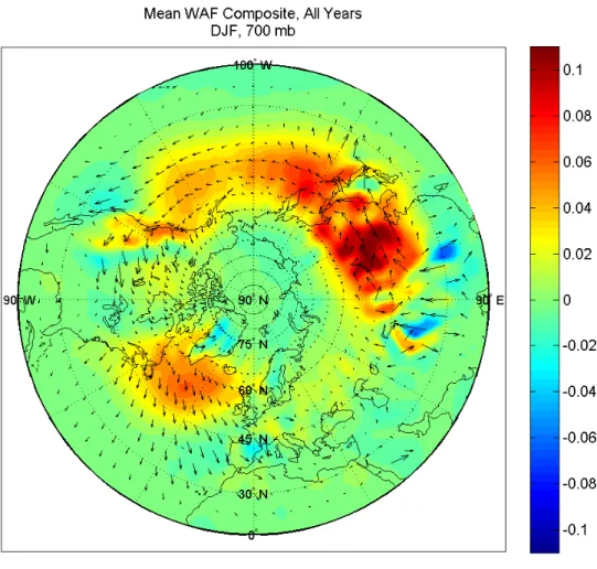
snow extents . . . 45 6.1 Mean winter wave activity flux over the Northern Hemisphere

(9)

6.2 Profiles of mean wave activity flux at 30N latitude from 30E to 150E longitude and varying pressure levels during late December and early January following Octobers with anomalously high

Eurasian snow extents . . . 49

6.1 Profiles of mean wave activity flux at 30N latitude from 30E to 150E longitude and varying pressure levels during late December and early January following Octobers with anomalously low Eurasian snow extents . . . 50

6.4 Hemispheric maps of geographical areas with mean vertical wave activity flux anomalies at 150 mb significant at the 90% and 95% confidence levels for late December and early January following anomalous October snow extents . . . .51

6.5 Hemispheric maps of geographical areas with mean vertical wave activity flux anomalies at 50 mb significant at the 90% and 95% confidence levels for late December and early January following anomalous October snow extents . . . .52

A.1 Fall (SON) EOF1 patterns for different pressure levels . . . .56

A.2 Winter (DJF) EOF1 patterns for different pressure levels . . . 57

A.3 Spring (MAM) EOF1 patterns for different pressure levels . . . .58

A.4 Summer (JJA) EOF1 patterns for different pressure levels . . . 59

B.1 Mean NH surface pressures from January 1949 to May 2008 . . . 60

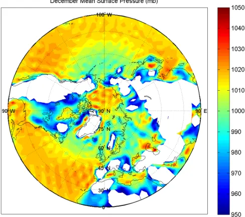
B.2 Mean December NH surface pressures from 1949 to 2007 . . . 61

C.1 September significant geopotential anomaly areas prior to anomalous snow extents, at 1000 mb, 700 mb, and 500 mb . . . 63

C.2 September significant geopotential anomaly areas prior to anomalous snow extents, at 250 mb, 150 mb, and 50 mb . . . 64

C.3 October significant geopotential anomaly areas following anomalous snow extents, at 1000 mb, 700 mb, and 500 mb . . . 65

C.4 October significant geopotential anomaly areas following anomalous snow extents, at 250 mb, 150 mb, and 50 mb . . . 66

C.5 November significant geopotential anomaly areas following anomalous snow extents, at 1000 mb, 700 mb, and 500 mb . . . 67

C.6 November significant geopotential anomaly areas following anomalous snow extents, at 250 mb, 150 mb, and 50 mb . . . 68

(10)

C.7 December significant geopotential anomaly areas following

anomalous snow extents, at 1000 mb, 700 mb, and 500 mb . . . 69 C.8 December significant geopotential anomaly areas following

anomalous snow extents, at 250 mb, 150 mb, and 50 mb . . . 70 C.9 January significant geopotential anomaly areas following

anomalous snow extents, at 1000 mb, 700 mb, and 500 mb . . . 71 C.10 January significant geopotential anomaly areas following

anomalous snow extents, at 250 mb, 150 mb, and 50 mb . . . 72 C.11 February significant geopotential anomaly areas following

anomalous snow extents, at 1000 mb, 700 mb, and 500 mb . . . 73 C.12 February significant geopotential anomaly areas following

anomalous snow extents, at 250 mb, 150 mb, and 50 mb . . . 74 E.1 Early November mean WAF anomalies vertical zonal profile

following anomalous snow extents . . . .78 E.2 Late November mean WAF anomalies vertical zonal profile

following anomalous snow extents . . . .79 E.3 Early December mean WAF anomalies vertical zonal profile

following anomalous snow extents . . . .80 E.4 Late December mean WAF anomalies vertical zonal profile

following anomalous snow extents . . . .81 E.5 Early January mean WAF anomalies vertical zonal profile

following anomalous snow extents . . . .82 E.6 Late January mean WAF anomalies vertical zonal profile

following anomalous snow extents . . . .83 E.7 Early February mean WAF anomalies vertical zonal profile

following anomalous snow extents . . . .84 E.8 Late February mean WAF anomalies vertical zonal profile

following anomalous snow extents . . . .85 F.1 Early November significant WAF anomaly areas following

anomalous snow extents, at 700 mb . . . . . . 86 F.2 Early November significant WAF anomaly areas following

anomalous snow extents, at 500 mb, 250 mb, and 150 mb . . . 87 F.3 Early November significant WAF anomaly areas following

anomalous snow extents, at 50 mb, and late November at

(11)

F.4 Late November significant WAF anomaly areas following

anomalous snow extents, at 250 mb, 150 mb, and 50 mb . . . 89 F.5 Early December significant WAF anomaly areas following

anomalous snow extents, at 700 mb, 500 mb, and 250 mb . . . 90 F.6 Early December significant WAF anomaly areas following

anomalous snow extents, at 150 mb and 50 mb, and late

December at700 mb . . . 91 F.7 Late December significant WAF anomaly areas following

anomalous snow extents, at 500 mb, 250 mb, and 150 mb . . . 92 F.8 Late December significant WAF anomaly areas following

anomalous snow extents, at 50 mb, and early January at

700 mb and 500 mb . . . 93 F.9 Early January significant WAF anomaly areas following

anomalous snow extents, at 250 mb, 150 mb, and 50 mb . . . 94 F.10 Late January significant WAF anomaly areas following

anomalous snow extents, at 700 mb, 500 mb, and 250 mb . . . 95 F.11 Late January significant WAF anomaly areas following

anomalous snow extents, at 150 mb and 50 mb, and early

February at700 mb . . . 96 F.12 Early February significant WAF anomaly areas following

anomalous snow extents, at 500 mb, 250 mb, and 150 mb . . . 97 F.13 Late February significant WAF anomaly areas following

anomalous snow extents, at 700 mb, 500 mb, and 250 mb . . . 98 F.14 Late February significant WAF anomaly areas following

(12)

List of Tables

4.1 Winters preceded by seven highest and lowest mean snow cover anomalies over Eurasia in October and their respective

(13)

Chapter 1 Introduction and motivation

The weather of the extratropics in the Northern Hemisphere (NH) is most severe during winter months. Europe and northeastern North America are particularly prone to fluctuations of the severity of winter weather from year to year. Unfortunately, weather prediction on timescales greater than a couple of weeks is very poor for the North Atlantic region. The large variability of air temperatures and the frequency and intensity of winter storms therefore pose formidable challenges to the socio-economic sectors of these densely populated regions of the world. With little warning of what weather each winter will bring, the planning of the allocation of resources necessary for adequately coping with the winter climate with minimal cost is exceedingly difficult.

Scientists have long known that winter surface climate over Europe and the northeastern parts of North America are strongly influenced by the Arctic Oscillation (AO). The AO, like the more well-known El Nino/Southern Oscillation (ENSO), is an atmospheric mode of variability describing the large-scale state of the atmosphere. While ENSO largely accounts for the fluctuations of climate in the tropics, the AO explains much of the variance of the atmosphere in the extratropical Northern Hemisphere. The predictive skill of the AO, however, is not as good as that of ENSO. While ENSO is closely correlated with the

temperature of the Pacific Ocean, a water body with very high thermal inertia, the AO is an internal mode, largely independent of forcings external to the atmosphere, and therefore much more difficult to predict.

Research over the past couple decades, however, has demonstrated that the AO can be modulated by external conditions, such as ocean temperatures and the cryosphere. In particular, there is good evidence suggesting a significant relationship between snow cover over Eurasia in autumn and the atmospheric state in the Northern Hemisphere in winter. A dynamical pathway from surface snow conditions to the winter NH circulation involving the propagation of stationary planetary waves and coupling between the troposphere and the stratosphere has also gained considerable credence. The possibility that an external measurable condition, such as snow extent, precedes winter conditions on seasonal

(14)

timescales brings hope of improving the predictive skill for the AO and winter weather over the North Atlantic regions.

While researchers have explored the relationship between snow extent and winter climate in both modeling and observational studies in the past, and have proposed a model for the dynamic mechanism linking the two phenomena, results have been limited by a trade-off between quality and quantity of available atmospheric data. The sensitivity of variability of winter climate and snow cover require many decades of reliable data to assess meaningful relationships between them. Atmospheric data sets extending back in time to before the 1970s have been derived using either outdated data assimilation methods or different data assimilation methods for different time periods, and are therefore not particularly reliable. Data sets derived consistently with one modern data assimilation method are more ideal. Until recently, however, such high quality data sets have not had large temporal ranges.

The following thesis presents observational work investigating the relationship between autumn snow extent over Eurasia and winter climate dynamics in the Northern Hemisphere using results of the ERA-40 Project. Released in 2007 by the European Centre for Medium-range Weather Forecasting, the ERA-40 Project is the result of the most recent large-scale re-analysis project incorporating multiple observational data sets and modern assimilation models. It has been deemed an improvement upon previous sets of global atmospheric data (Uppula, et al. 2005). Spanning from August 1957 to September 2002, it has a temporal range superior to other atmospheric data sets of similar caliber, enabling it to yield the most reliable results to date for the relationship between anomalous autumn

Eurasian snow extent and the winter AO mode.

The research presented in this thesis seeks to answer several questions. First, is the correlation between October snow extent over Eurasia and the climatic conditions during the following winter found in previous studies a result of atmospheric persistence alone? Second, given that snow and atmospheric circulation both vary on decadal timescales, are the relationships between autumn snow and winter climate reported in the literature artifacts of short records of data? Last, is the dynamic pathway between snow and the Arctic Oscillation proposed in previous studies statistically significant?

The thesis will be structured in the following way. An overview of climate science and a literature review of previous related work done will be introduced to the reader in Chapter 2. Chapter 3 will present and discuss the Arctic Oscillation (AO) seasonal

teleconnection patterns and the evolution of the AO from 1957 to 2002. An analysis and discussion of October Eurasian snow extent data and the identification of anomalous snow years will follow in Chapter 4. In Chapter 5, a significant relationship between anomalous autumn snow extent and the winter phase of the AO will be demonstrated. Chapter 6 will

(15)

present evidence supporting a dynamic pathway between surface snow conditions and the winter zonal mean circulation. Finally, a summary of results and concluding remarks will appear in Chapter 7.

(16)

Chapter 2 Background

The following chapter introduces the topics of climate science and atmospheric dynamics and provides a review of previous research relevant to this thesis. It starts with a background in the dynamics of the atmosphere, focusing on the troposphere, stratosphere, and interactions between them via planetary waves. Next, atmospheric variability is discussed with particular emphasis on the Arctic Oscillation. Finally, the surface energy balance of snow as well as research work on the relationship between snow and climate are presented.

2.1 Atmospheric dynamics

2.1.1 The Troposphere and the Stratosphere

The troposphere and the stratosphere are the two layers of the atmosphere closest to the Earth’s surface. The troposphere is the bottom layer of the atmosphere, spanning vertically from the Earth’s surface to anywhere from 5 km above sea-level over the poles to 18 km above sea-level over the tropics. As the densest layer of the atmosphere, it contains approximately 80% of atmospheric mass and is the only region of the atmosphere in which clouds and precipitation occur. Air pressure in the troposphere decreases logarithmically with elevation, from around 1000 mb at sea-level to near 250 mb at the top. The stratosphere is located above the troposphere, separated from it by the thin tropopause. It extends from near the top of the troposphere to between 40 and 50 km above mean sea-level, with air pressures around 250 mb at the bottom, 150 mb near the middle, and 50 mb at the top.

The troposphere is the boundary layer between the atmosphere and the Earth’s surface and is the most turbulent layer of the atmosphere. Its turbulence is indicative of a high level of baroclinicity which is the result of a complex combination of external forcings: mechanical forcing from orography, thermal forcing from land-sea interactions and the

(17)

cryosphere, radiative forcing from the sun, and physical forcing due to the rotation of the Earth. The troposphere is particularly turbulent in the extratropics, where the variability of solar radiation is largest and the effects of the rotation of the Earth on air flow trajectories are most pronounced. In these regions, the circulation of the troposphere is highly asymmetric about the pole, dominated by regional cyclonic systems, including both counter-clockwise rotating cyclones and clockwise rotating anti-cyclones, characterized by low and high pressure systems respectively.

Peak turbulence in the Northern Hemisphere (NH) extratropics occurs in winter when atmospheric thermal gradients are maximal. While the extratropical oceans remain relatively warm in winter due to the high thermal inertia of large bodies of water, the continental land masses become relatively cold with the seasonal drop in solar heating. In addition, the differences in insolation between the tropics and the pole are greatest in winter. Both of these phenomena result in the strongest latitudinal and meridional thermal gradients over the mid to high latitudes of the entire year. Winter is therefore also the time of the most severe climate for the Northern Hemisphere extratropical regions, with particularly strong cyclones, such as the classic Nor’easters over North America, and anticyclones, such as the extremely cold Siberian High over Eurasia.

The stratospheric atmosphere lies above the turbulent realm of precipitation and most storms and is largely barotropic, meaning its air density is dependent only on air pressure. As primarily barotropic, the stratosphere is in approximate hydrostatic equilibrium and is therefore quite stable. In the Northern Hemisphere, the circulation in the stratosphere is governed chiefly by the polar vortex and is characterized by the zonal jet which circles roughly symmetrically around the pole. Associated with the zonal jet is the zonal wind which is strongest in the extratropics during winter months when westerlies dominate the stratospheric flow.

While the polar vortex and the zonal wind are primarily stratospheric phenomena, they can influence the circulation and climate of the troposphere through downward coupling between the two layers. Disruptions to the strength of the polar vortex result in changes in the mean zonal wind flow, affecting the circulation below. Several studies have attributed tropospheric conditions to changes in the stratospheric circulation. Hartley et al (1998) showed that disruption of the polar vortex in the Northern Hemisphere stratosphere during winter significantly influences the climate of the upper troposphere. Using observational data, Thompson et al. (2001) showed that a weakening of the polar vortex affects surface weather resulting in a greater frequency of severe cold events over the North Atlantic and East Asia. In a modeling study, Scaife et al. (2005) concluded that downward coupling between the stratosphere and the troposphere accounts for most of the

(18)

variance in surface climate in the North Atlantic region from 1965 to 1995.

2.1.2 Planetary waves

Most disruptions to the polar vortex are caused by atmospheric coupling between the stratosphere and the troposphere, through the upward propagation of planetary waves from the troposphere to the stratosphere. Atmospheric waves of many different wavelengths and directions pervade the atmosphere. However, the direction and strength of the zonal wind place limitations on which waves can successfully propagate vertically and how far they can travel. Generally, waves with longer wavelengths are able to propagate further in the presence of stronger westerlies in the atmosphere (Serreze and Barry, 2005). Wintertime, when the zonal mean wind is strongest, is therefore the optimal time for the vertical

propagation of planetary waves. Indeed, conditions are most favorable during this time for particularly strong planetary waves with long wavelengths, on the order of half of the zonal perimeter, to penetrate into the stratosphere and weaken the polar vortex.

Planetary waves originate in the troposphere and can be enhanced or dampened near the surface where orographic and thermal forcings are present (Chen and Trenberth 1988, Plumb 1985). Thermal gradients set up by surface conditions, such as sea ice, snow cover, and sea surface temperatures (SST), are a source of baroclinicity and thereby affect wave production. Similarly, mountains affect wave production by effectively disrupting horizontal air flow and creating local pressure gradients.

The modulation of planetary waves is greatest in the presence of both thermal gradients and mountains. The impacts of diabatic forcing and orography on planetary waves are non-linear, with the effects of both thermal and mechanical forcing together greater than the sum of their individual contributions (Ringler and Cook 1988). Differences also exist between the effects of diabatic heating and cooling on both planetary wave and cyclonic activity. While the presence of diabatic heating and orography together enhance cyclonic activity and dampen the upward propagation of waves, diabatic cooling and orography together enhance both anti-cyclonic systems and upward wave production (Chen and

Trenberth 1988, Ringler and Cook 1998). The likelihood of enhanced upward vertical wave propagation is therefore greatest over mountainous and cold regions.

For this reason, the region of greatest vertical wave propagation is Eurasia. Eurasia is the largest contiguous land mass on the planet and is home to the most extreme and variable surface conditions in the extratropics of the NH. The continent is shielded from relatively warm ocean air by Europe to the west and its air flow is blocked to the south and

(19)

east by numerous mountain ranges, including the towering Tibetan Plateau, extending to the highest elevations on the planet. This unique geography enables the growth of the Siberian High, the massive high pressure system that dominates the region’s winter climate, making Siberia the coldest and harshest place on Earth during winter months, and also the largest source of vertically propagating stationary waves.

2.2 Modes of variability

2.2.1 Teleconnection patterns

While the atmosphere is constantly in chaotic and turbulent flux on short timescales of days and weeks, close scrutiny of large-scale variability reveals recurring patterns in the relationships between the atmospheric states of different geographical regions on much greater timescales. These observed patterns of variability occur with low

frequencies, on the order of months to decades (Barnston and Livezey 1987), and are referred to as teleconnection patterns. Defined by Wallace and Gutzler (1981) as the

“contemporaneous correlation between geopotential heights on a given pressure surface at widely separated points on Earth,” teleconnection patterns essentially show the simultaneous variability between distant parts of the globe. They can be derived for different regions of the globe using different points of reference for correlation and feature “centers of action,” geographical areas where co-variability is largest. Robust patterns that are consistently replicated using different methods are known as atmospheric modes of variability.

There are multiple modes of variability that are well-documented for the Earth’s atmosphere, with the most well-known being the El Niño/Southern Oscillation. ENSO is a tropical phenomenon that is characterized by an oscillation between two extreme

atmospheric states, El Niño and La Niña, with a period ranging from two to seven years (Ahrens, 2009). Each phase of ENSO greatly impacts surface climate across the globe, particularly over tropical locations. An El Niño event, for example, is accompanied by a greater frequency of typhoon development over the tropical central Pacific, a weakening of Indian monsoons, and the development of fewer hurricanes over the tropical Atlantic Ocean (Ahrens, 2009).

Though ENSO is an atmospheric mode of variability, it is the result of coupling between the atmosphere and the ocean. Variability of ENSO is significantly correlated with variability of surface temperatures of the Pacific Ocean. El Niño is associated with a

(20)

surface waters over the central and eastern parts of the tropical Pacific. Because the thermal inertia of oceans is very high, observations of sea surface temperatures allow very skilled prediction of the phases of ENSO and their anticipated weather patterns months in advance.

There are many lesser known modes of variability outside of the tropics that have also been identified. These include the Pacific/North American Mode (PNA), the Eurasian Mode (EUR), the Northern Annular Mode (NAM), the North Atlantic Oscillation (NAO), and the Arctic Oscillation (AO). Meteorologists have been aware of the NAO for the longer than all of the other modes of variability. First identified by Walker and Bliss in 1932, it is characterized by a north-south oscillation of atmospheric mass over the North Atlantic, is strongest in winter, and affects weather over the North Atlantic region (Walker and Bliss 1932, van Loon and Rogers 1978). Other patterns have emerged as mathematical techniques for identifying patterns of variability have been improved. The PNA features centers of action over the North Pacific and the western and eastern parts of the United States and is most pronounced at the 500 mb pressure level. The EUR is similar in influence to the PNA but is characterized by a center of action over Eurasia. The NAM and AO are largely

symmetric about the origin and strongly resemble one another, except in winter when the AO features a pressure dipole over the North Atlantic similar to the NAO.

There is some confusion in the literature regarding the differences, if any, between the AO, NAO, and NAM modes. The surface manifestation of the AO in

wintertime strongly resembles the NAO pattern. It is thus sometimes used interchangeably with the NAO. The AO is also thought to potentially have the same underlying mechanisms as the Northern Annual Mode (NAM) (Vallis et al. 2004). In this thesis, I will refer only to the AO with the implicit understanding that the regional NAO generally dominates the hemispheric AO during wintertime in the Northern Hemisphere and the AO and the NAM are potentially the same mode.

2.2.2 Arctic Oscillation

The Arctic Oscillation is the dominant mode of variability in the mid to high latitudes of the Northern Hemisphere. It is a barotropic mode and exists separately from the turbulence of the troposphere. The AO is strongest during winter and extends from the surface to the stratosphere during this time (Thompson and Wallace 1998, Baldwin and Dunkerton 1999). The AO teleconnection pattern in winter features two oppositely signed centers of action over the northern Atlantic Ocean. The surface manifestation of the AO is characterized by a pressure dipole with a low pressure system over the North Atlantic basin

(21)

off the western coast of Iceland and a relatively high pressure system over Azores to the south whose strengths vary negatively with each other (Wallace and Gutzler 1981, Thompson and Wallace 1998).

The strength of the winter AO, measured by the strength of the pressure gradient over the North Atlantic and also referred to as the AO phase, impacts surface weather, including temperature distribution, precipitation intensity, and storm frequency, over densely populated North Atlantic regions (Walker and Bliss 1932; van Loon and Rogers 1978; Serreze et al. 1997). In the positive phase, the pressure gradient between the two centers of action is particularly strong, resulting in anomalous westerlies over the Atlantic Ocean, warmer than normal temperatures over Europe and the eastern United States, colder

temperatures over the northwestern part of the Atlantic, and a shift of storm tracks north over Europe. Conversely, the negative phase is characterized by a particularly weak pressure gradient, and is accompanied by anomalous easterlies, an opposite trend in temperatures, and more storm activity over Western Europe and the northeastern parts of the United States (Hurrell et al. 2003).

The AO is an internal mode of the atmosphere, meaning its existence is a result of the physics of the atmosphere alone, not a product of coupling of the atmosphere with surface conditions as is the case with ENSO. Internal variability of the atmosphere alone, however, fails to explain all of the inter-annual variance of the AO mode over the past several decades (Feldstein 2002). Recent studies have suggested, however, that while external forcings at the surface do not cause the AO, anomalous conditions external to the atmosphere may modulate the strength of the AO, accounting for the unexplained variance (Kodera and Yamazaki 1994, Kodera 1995, Gong et al. 2002). Extreme surface conditions may serve as pathway “triggers,” influencing the progression to a particular phase of the AO given the right conditions (Cohen et al. 2002).

Multiple surface conditions have been linked with the atmospheric circulation and climate to varying degrees. Examining the influence of snow depth, Lu (2008) found a correlation between snow depth over the Tibetan Plateau and the winter Arctic Oscillation. Variability of sea surface temperatures and atmospheric circulation in the Northern

Hemisphere has been shown to be correlated on both interannual and interdecadal timescales (Kushnir 1994, Robertson et al. 2000). Further studying SSTs, Saunders and Qian (2002) showed that sea surface temperatures can predict the NAO winter phase weeks in advance with mild success. In addition to snow depth and SSTs, sea ice extent has also been studied. Murray and Simmons (1995) demonstrated that a decrease in sea-ice extent in the past can be linked with weakening westerlies and lower tropospheric warming, and Wang and Ikeda (2000) showed that fluctuations of sea ice are correlated with changes in the Arctic

(22)

Oscillation. Ross and Walsh (1986) looked at the effects of both sea ice and snow cover on local temperatures determining both could be used for short-term forecasting over the United States. Also studying snow cover, Watanabe and Nitta (1998) found that abrupt changes in the winter atmosphere were preceded by anomalous snow cover extents over Eurasia and Cohen and Entekhabi (1999) demonstrated a correlation between Eurasian snow cover in fall and the strength of the winter zonal mean wind.

Of all of the external surface conditions that have been studied for their relationship with the atmosphere, snow extent has received the most attention. While correlations exist between climate and sea surface temperatures, sea ice, and snow depth, their respective lag times are not as great as that for the correlation between snow extent and the winter atmosphere. Snow extent is therefore the strongest contender to serve as a skillful predictor of the winter AO phase.

2.3 Snow and climate

Snow has long been known to influence local climate. Local surface temperature and snow cover variability are significantly correlated, with snow cover reducing local air temperatures (Namias 1962, Dewey 1977, Walsh et al. 1982). The net effect on local temperatures is due to the different physical properties of snow and land. The higher albedo of snow results in a greater percentage of incident short-wave radiation reflected and less solar heat absorbed. More long-wave radiation is lost due to the higher thermal emissivity of snow. In addition, snow cover has a lower thermal conductivity than soil, insulating the ground and suppressing sensible heat flux from the ground to the air. Lastly, the melting of snow acts as a latent heat sink, absorbing heat from the air locally.

While the effects of snow on local temperatures have been documented for many decades, the relationship between snow cover and climate on larger scales has only been explored more recently. Hoskins and Karoly (1981) opened the door to such research by showing that the internal dynamics of the atmosphere may propagate local surface

temperature anomalies, such as those produced by snow, to remote distances, enabling local thermal anomalies to impact the general circulation on larger scales. In addition, snow cover interannual variability has been linked with hemispheric atmospheric variability, and

anomalous continental snow cover has been shown to influence NH surface climate in winter (Gutzler and Rosen 1992, Walland and Simmons 1997).

Snow cover over the Eurasian continent in particular has emerged as having a relationship with atmospheric circulation. Anomalous snow cover over Eurasia in spring has

(23)

been significantly linked with the strength of the Southeast Asian monsoon and the general atmospheric circulation of East Asia (Barnett 1989, Clark and Serreze 2000). Most notable, however, has been the evidence that Eurasian snow cover in autumn affects the winter climate of the region. Significant correlations between autumn Eurasian snow extent and winter Eurasian surface temperatures, remote pressure levels, and the zonal mean wind have all been demonstrated in observational studies (Foster 1983, Walsh and Ross 1988, Cohen and Entekhabi 1999, Cohen et al. 2001).

In particular, a growing body of literature has linked the AO with autumn Eurasian snow cover. Saito et al. (2003) performed an observational study in which a significant correlation between Eurasian autumn snow extent and the winter AO was

discovered from 1971 to 2001. Cohen and Entekhabi (2001) used general circulation models (GCM) to show that the NH winter atmospheric circulation incorporating Eurasian snow cover as a boundary condition strongly resembled the AO mode. Gong et al (2002) also used GCMs to demonstrate that imposing significant autumn snow cover over Siberia resulted in AO signals originating in the fall over Siberia. Another modeling study concluded that the impact on the AO using significant snow extent over North America was not comparable to that using Siberian snow cover extent (Gong et al., 2003).

A dynamical pathway involving the diabatic cooling of snow cover, the production of stationary planetary waves, and the coupling of the troposphere and the stratosphere is the leading theoretical mechanism linking autumn Eurasian snow extent and the winter AO. Cohen et al. (2002) postulate that diabatic cooling from extensive snow cover over Eurasia can enhance vertical wave propagation, thereby triggering a dynamic pathway involving the penetration of tropospheric planetary waves into the stratosphere, a weakening of the polar vortex, a deceleration of the zonal mean flow, and a consequent downward refraction of the zonal flow anomaly from the stratosphere to the surface. In this way, the anomalous thermal cooling associated with anomalous snow extent in autumn, the season of largest snow extent variability, may trigger an internal atmospheric mechanism and modulate the wintertime strength of the AO.

(24)

Chapter 3 The Arctic Oscillation

Atmospheric variability in winter in the Northern Hemisphere extratropics is dominated by the Arctic Oscillation (AO). Fluctuations in the strength of the AO often mirror fluctuations in the mean state of the atmosphere in time. Because the AO phase in winter has important implications for surface conditions over Europe, eastern North

America, and parts of the Mediterranean, understanding the variability of the atmosphere in space and time is vital for improvements in predictive skill.

In this chapter, variability of the AO mode and the NH atmosphere in winter are assessed for the period of September 1957 to August 2002. The seasonal teleconnection patterns of the AO and general patterns of co-variability of different levels of the atmosphere are derived and presented with a discussion of methods used. The percentage of variance explained by each teleconnection pattern is shown to be greatest in January for all pressure levels. A seasonal and monthly index time series of the AO and the mean state of the atmosphere are described and the variability of the mean state of the atmosphere in winter over forty-five years is discussed. Finally, correlations between atmospheric indexes of consecutive months are calculated and conclusions about atmospheric memory are presented.

3.1 Teleconnection patterns

3.1.1 Sea-level

Atmospheric teleconnection patterns are derived using empirical orthogonal function (EOF) analysis. EOF analysis, also referred to as principle component analysis (PCA), is a mathematical method developed in the twentieth century to capture covariability of data with both spatial and temporal dimensions. The substantial correlations between atmospheric data on very large spatial and temporal scales make EOF analysis particularly useful for the study of atmospheric variables. Empirical orthogonal functions are defined as

(25)

the orthonormal eigenvectors of the correlation matrix of time- and space-varying data. The eigenvector with the largest eigenvalue captures the majority of variance of the data field. It is possible to derive teleconnection patterns by decomposing a spatial field of time series data into EOFs and mapping the ones with the greatest eigenvalues onto spatial fields.

The teleconnection pattern of the Arctic Oscillation is defined as the first empirical orthogonal function of sea-level pressure in the Northern Hemisphere. In the absense of sea-level pressure data, geopotential height anomalies at the 1000 mb pressure level may be used The geopotential height is the gravitational potential energy per unit mass of a given pressure level divided by the standard gravity at mean sea-level. It represents the vertical distance above mean-sea level at which the air pressure is equivalent to the pressure level of interest. Co-variability of geopotential heights for a constant pressure level are indicative of co-variability of atmospheric pressure and the general circulation of the atmosphere. Geopotential heights at 1000 mb, approximately mean sea-level, display the

Figure 3.1: Seasonal AO teleconnection patterns for September 1957 to August 2002 computed as the first empirical orthogonal functions of geopotential heights at 1000 mb.

(26)

same variability as sea-level air pressures and therefore can be used in EOF analysis to determine the AO teleconnection pattern.

The first EOF of each season was found using the mean seasonal geopotential anomalies for the period September 1957 to August 2002. Mean seasonal geopotential height anomalies were calculated using mean monthly geopotential height data provided in the ECMWF (European Centre for Medium-range Weather Forecasting) ERA-40 Reanalysis Project data set. Data points represent mean geopotential heights over a 5 degrees latitude by 5 degrees longitude grid. Seasons are defined as three month intervals; September, October, and November (SON) for fall, December, January, and February (DJF) for winter, March, April, and May (MAM) for spring, and June, July, and August (JJA) for summer. Because the AO is largely an extratropical phenomenon, only data from 20 degrees latitude to the pole in the Northern Hemisphere was included in this analysis and all analyses that follow in this thesis.

The AO seasonal teleconnection patterns are shown in Figure 3.1. Areas of color indicate regions of high variability, with the darkest shadings indicating areas in which variability is largest. Blue and red regions illustrate how the atmospheric states over these regions vary with each other; areas of the same color positively co-vary while regions that are opposite in color co-vary negatively. For instance, the fall EOF1 pattern features a red area over the Arctic and several areas of blue over the mid-latitudes, particularly over Northern Europe and the northern part of the Pacific Ocean. The variability of these areas explains the majority of the variance of the geopotential heights during the fall period with pressure anomalies over the Arctic and mid-latitude regions tending to occur simultaneously and with opposite sign.

The most prominent feature common to all AO seasonal patterns is the negative co-variability of atmospheric pressure over the Arctic and the mid-latitude regions. While the highly variable region over the Arctic is fairly symmetric around the pole, the areas of greatest variability in the mid-latitudes are highly asymmetric. Largest negative

co-variability of atmospheric pressure between the Arctic and the mid-latitudes occurs between the pole and two “centers of action,” one over the Atlantic Ocean and continuing onto the European continent and the other over the North Pacific, most prominently during fall and spring. The winter AO pattern is characterized by a pressure dipole with “centers of action” over the Atlantic basin east of Greenland and off the coast of Spain. This pattern indicates the tendency for simultaneous and opposite variability of the geopotential heights over the dipole centers; when the geopotential heights over one center become elevated, those over the other become depressed. The net effect is a fluctuation in the strength of the north-south pressure gradient in the region.

(27)

3.1.2 Other pressure levels

While the AO pattern is defined by variability at the surface, patterns of variability at pressure levels above the surface are useful for identifying the extent of the influence of the AO as well as other areas of co-variability in the atmosphere. Seasonal teleconnection patterns were derived for pressure levels beyond mean sea-level pressure, from 700 mb in the troposphere to 50 mb in the stratosphere. The patterns show

asymmetrical centers of action similar to those of the AO and which are strongest at 500 mb. In winter, the pressure dipole of the AO pattern persists up to the mid-stratosphere, indicating the far-reaching impact of the AO on the atmospheric state during this period. While most tropospheric patterns are highly asymmetrical, patterns in the stratosphere are symmetrical about the pole except in winter, with little if any negative covariance between the Arctic and

Figure 3.2: Interpolated contour plot of percentage of geopotential height variance explained by first empirical orthogonal function of mean seasonal geopotential heights at varying pressure levels.

(28)

mid-latitude areas. Figures of seasonal teleconnection patterns can be found in Appendix A.

The teleconnection pattern of each season does not explain all of the variation of the geopotential height anomalies. As mentioned in section 3.1.1, information about the amount of variance captured by each pattern lies in the eigenvalue of the first EOF. Figure 5.2 shows an interpolated contour plot of the percentage of variance of geopotential

variability explained by the first EOF for different pressure levels and seasons. The figure clearly shows the dominance of the first EOF during winter extending from the surface, throughout the troposphere, and into the stratosphere. The winter AO pattern explains 34.5% of the variability of the winter (DJF) geopotential anomalies at 1000 mb, the largest

percentage of variability explained for the troposphere and lower stratosphere over all

seasons. In addition, with the exception of the upper stratosphere, the percentage of variance explained by the first EOF is greatest in winter for all pressure levels analyzed. This trend indicates the dominance of the Arctic Oscillation mode in atmospheric variability during winter months.

3.2 Evolution of the AO

While the AO teleconnection patterns show co-variability of the atmospheric state in space and time, they do not give any information about periods of fluctuation. To assess how the strength of the AO and the general state of the atmosphere vary in time, monthly and seasonal indexes were developed to represent the contribution of each year to the variability patterns.

Each index time series spans forty-five years and is based on the first empirical orthogonal function for a specific time period and pressure level. Each index is found by projecting a vector of mean geopotential anomalies for a fixed time period of a given year onto the first EOF eigenvector. The series of indexes that result from the projections of anomalies of all years onto the first EOF are normalized, yielding an index time series with zero mean and unit standard deviation.

The index time series for winter (DJF) at 1000 mb represents the fluctuation of the annual strength of the AO. The series is plotted in Figure 2.3 with years shown

corresponding to December of the winter of each index. Strongly negative (positive) indexes indicate the negative (positive) phase of the AO. The 1976-1977 winter stands out as

featuring an exceptionally strong negative phase of the AO while a strongly positive phase occurred during winter of 1988-1989. The AO index time series also shows a general shift from mostly negative AO phases prior to the late 1980s to mostly positive phases afterwards.

(29)

Figure 3.3: Winter EOF1 index time series for 1000 mb geopotential heights. Winters span December of the year indicated to February of the following year.

This phenomenon has been noted by researchers in the past and has largely been theorized to be caused by interdecadal variation, although the increasing concentrations of greenhouse gases in the atmosphere are also theorized by some to be a factor.

3.3 Atmospheric persistence

Correlations between consecutive indexes of a given EOF1 index time series enable an assessment of memory in the atmosphere. Because each index is representative of the mean state of the atmosphere, persistence of an index value for a given pressure level in time is indicative of atmospheric persistence. Understanding when and where atmospheric persistence is greatest improves the identification of potential skillful predictors of climate.

(30)

Figure 3.4: Intra-monthly correlations of EOF1 monthly indexes for different pressure levels. Monthly indexes are based on monthly mean geopotential height anomalies from September 1957 to August 2002. White areas show where correlations are insignificant from zero.

To assess the persistence of the atmospheric state on monthly timescales, monthly EOF1 indexes were developed based on the first empirical orthogonal functions of mean monthly geopotential heights for various pressure levels. For each pressure level, intra-monthly correlations of the monthly index time series were computed and significance testing of the correlation was performed. Figure 3.4 shows an interpolated plot of all

correlations significantly different from zero.

As the figure shows, there is a notable difference in atmospheric persistence between the troposphere and the stratosphere. While there are significantly high correlations between consecutive monthly indexes in the stratosphere, particularly during summer months and from late fall into winter, persistence in the troposphere is limited to winter months and a brief period during the summer. The stability of the barotropic stratosphere accounts for the

(31)

high level of atmospheric memory in the stratospheric layer, with particularly high correlations in summer likely due to the general uniformity of the NH stratosphere in summer when the polar vortex is stable and the stratosphere approaches radiative equilibrium. In contrast, the relatively few periods of significant correlations in the troposphere result from a high level of baroclinicity.

The atmospheric memories of the stratosphere and the troposphere from early fall to late winter have particular relevance to prediction of the AO winter phase. The

insignificant tropospheric atmospheric memory throughout the fall months show no

atmospheric precursors to the winter AO in the troposphere during the fall. Once it has been established in December, however, persistence of the winter AO phase in the troposphere is seen over all winter months. In the stratosphere, however, persistence exists beginning in October and lasting until spring, though not very strongly. The weak stratospheric

persistence is likely due to the high stability of the stratosphere relative to the troposphere. The findings imply that while the mean monthly atmospheric states in the troposphere in fall may not predict the mean winter state of the atmosphere, those in the stratosphere beginning in November may, but to a very limited degree.

(32)

Chapter 4 Eurasian snow cover

The analysis of the variability of snow extent has historically been limited by inadequate or non-existent snow records. The examination of the variability and trends connected with years with anomalous snow cover is particularly susceptible to bias due to a lack of data points. Fortunately, work has been done over the past few decades to reconstruct a reliable historical snow extent time series for the globe based on data collected using both old and modern methods.

This chapter presents the snow data that were used for the research presented in this thesis. First, the history and challenges of snow data collection are discussed. Next, the snow data set used is introduced along with observations and comparisons with a data set incorporating more recent observations. Finally, years with anomalous snow extent, the topic of future chapters, are identified.

4.1 Snow Data

The extent of snow cover in the Northern Hemisphere has been documented remotely using satellite imagery since 1966 (Matson et al. 1986). The National Oceanic and Atmospheric Administration (NOAA) has compiled weekly satellite charts since that time with increasing resolution and accuracy as technology has advanced. However, certain challenges will always remain in interpreting real snow extent from satellite imagery, including the lack of data due to clouds, the difficulty in distinguishing between snow and clouds over mountainous areas, and the low visibility of snow over large, dense forests (Robinson 1993). While methodologies for estimating snow coverage were developed soon after satellite imagery became available, the methodology most widely regarded as best in quality was developed by Robinson in 1993. Robinson formulated a new algorithm to more accurately derive continental snow extent extending back in time to 1972. Also known as the Rutgers routine, Robinson's methodology is currently used by the Rutgers Snow Lab to

(33)

derive continental snow extent from incoming satellite data.

While remote sensing has enabled reliable estimations of snow extent over vast a areas of land for nearly four decades, snow cover data over an even longer period is desirable for the study of anomalous snow events. The more crude land-based observations of snow cover are thus essential for determining snow extent for years before widespread satellite use. While the earliest records of in situ observations of snow cover in the Northern Hemisphere date back over a century, the geographical areas they are available for are limited. In

addition, the data records contain many gaps in time. In the past decade, meteorologist Ross D. Brown has addressed these challenges by reconstructing monthly snow cover extent for much of North America and the Eurasian continent using historical records of in situ snow cover observations and reconstructed snow cover data. He was able to reconstruct snow

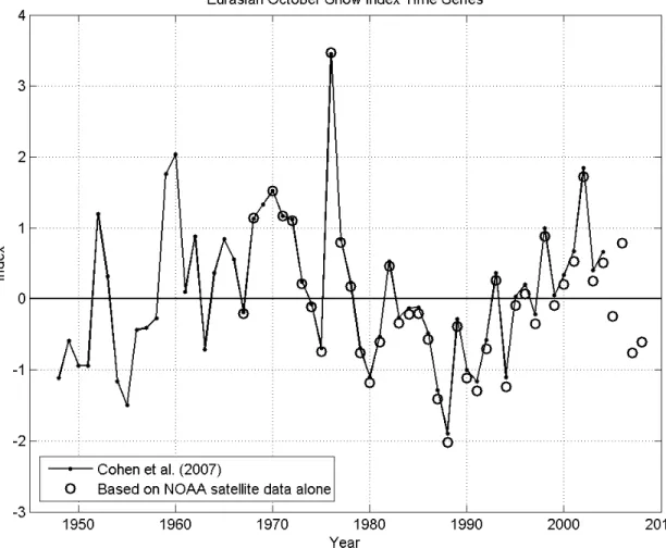
Figure 4.1: Comparison of two normalized index time series representing mean snow extent over Eurasia during October.

(34)

cover data for North America going back to 1915 for all months and for Eurasia going back to 1922 for October, March, and April (Brown 2000).

Cohen et al. (2007) combined both Robinson's analysis of satellite data and Brown's reconstruction of in situ snow cover observations to develop a time series of mean snow cover over Eurasia in October from 1948 to 2004. The data was normalized to yield an index time series with positive and negative values representing multiples of standard

deviations above and below average mean snow extents respectively.

To test the robustness of the data set, another index time series was calculated using a shorter time period but more recent snow cover values, and was compared with the longer index time series. The new series includes only satellite data, spans from October of 1967 to 2008 with the exception of 1969 when data was not available, and was collected

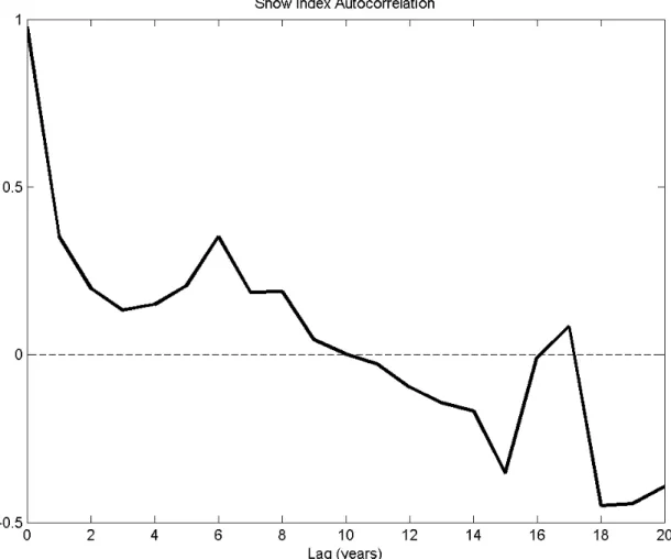
Figure 4.2: Autocorrelation of snow extent index time series derived by Cohen et al., 2007. The time series spans from 1948 to 2004.

(35)

entirely by NOAA and made available from the Snow Lab of Rutgers University. The two index time series are shown in Figure 4.1, with the indexes using only satellite data

represented as open circles and the indexes of the longer series by Cohen et al. (2007) connected by lines.

The autocorrelation of the longer time series is shown in Figure 4.2. The most pronounced variability of October Eurasian snow extent occurs with a frequency of about six years. There is a strong negative autocorrelation for indexes with a lag of around twenty years. Over the decades for which snow data is available, a shift from a tendency of positive snow indexes to negative is clearly displayed. This shift occurred in the late seventies to early eighties, approximately in the middle of the period over which snow data was considered.

The two series match very well until the 1990s in which the shorter satellite data indexes are markedly lower than the longer series index values, indicating the trend of decreased mean snow extent over the past few decades in comparison to the last sixty years. The observed change in average snow extent implies that one of the following is true: October snow extent varies on decadal timescales, changes in climate over the past twenty years have resulted in less snow, or both decadal variation and global change is occurring. It is certain that snow extent indeed varies on decadal timescales. Whether climate change is impacting snow extent or not, the decadal variability of snow makes using a long snow data set imperative in the study of the relationship between snow and the atmosphere. The index developed by Cohen et al. (2007), incorporating snow data going back to 1948, was thus used for all snow analyses presented in this thesis henceforth.

4.2 Anomalous snow years

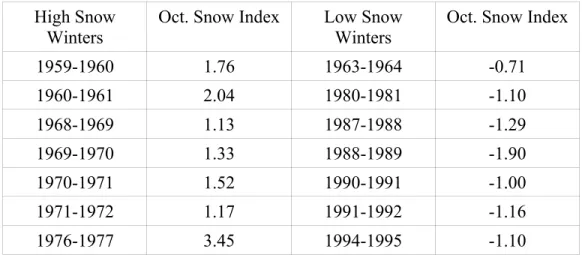
To study the relationship between anomalous snow extent in October and the atmospheric state of the following winter, fourteen Octobers with the most extreme snow extent indexes were chosen to represent years with anomalous autumn snow cover. A total of seven years of each extreme was chosen to minimize clustering while retaining a good spread of data points. The years chosen for analysis are shown in Table 4.1. Hypothesis testing shows that the mean anomalously high and low snow index sets are both significantly different from the mean index over all years with 95% confidence. Anomalous snow years referenced throughout the rest of this thesis refer to the seven highest and seven lowest indexes for the years shown in Table 4.1.

(36)

High Snow Winters

Oct. Snow Index Low Snow Winters

Oct. Snow Index

1959-1960 1.76 1963-1964 -0.71 1960-1961 2.04 1980-1981 -1.10 1968-1969 1.13 1987-1988 -1.29 1969-1970 1.33 1988-1989 -1.90 1970-1971 1.52 1990-1991 -1.00 1971-1972 1.17 1991-1992 -1.16 1976-1977 3.45 1994-1995 -1.10

Table 4.1: Winters preceded by seven highest (column 1) and lowest (column 3) mean snow cover anomalies over Eurasia in October and their respective snow indexes.

(37)

Chapter 5 Snow and the AO

The strength of the Arctic Oscillation in winter is difficult to predict months in advance because of the apparent lack of direct coupling between the atmosphere and any external parameters with large lag time. Evidence has emerged, however, that snow cover extent, acting as a large-scale thermal boundary condition for the NH atmosphere, may modulate the strength of the AO months in advance. In particular, anomalous fall snow extents may serve as skillful seasonal predictors of the winter AO phase.

This chapter presents observational evidence of a significant relationship

between October Eurasian snow extent and the mean state of the atmosphere in the Northern Hemisphere. The snow index presented in Chapter 4 and the EOF1 indexes described in Chapter 3 are compared and correlations are determined. Mean monthly composites of geopotential anomalies following anomalous October Eurasian snow extents are presented and analyzed, demonstrating a significant link between anomalous snow extent and the winter AO phase. Finally, trends in the mean stratospheric states in winters following anomalous October snow cover are discussed.

5.1 Autumn snow and the winter atmosphere

To quantify the relationship between mean October snow extent over Eurasia in the fall and the monthly mean state of the atmosphere over time, Pearson correlations were found between the snow index time series and the EOF1 monthly index for different pressure levels and months. An interpolated contour plot of the correlations between October snow and the EOF1 indexes for September through February is shown in Figure 5.1. Most noticeable is the sign of the correlations between the snow and atmospheric indexes: all correlations are negative. This indicates an inverse relationship between October snow extent and the atmosphere.

(38)

Figure 5.1: Interpolated contour plot of correlations between the mean October Eurasian snow index time series and different monthly EOF1 index time series for different pressure levels. The air pressure axis is scaled by elevation.

stratosphere, with maximum correlation occurring in the mid to lower stratosphere.

Correlations for January are significantly different from zero at the 99% confidence level for all pressure levels indicating a significant relationship between October snow extent over Eurasia and the state of the atmosphere from the surface to the upper stratosphere during January. In December, correlation between snow extent and the atmosphere is significant at the 99% level only in the stratosphere and is considerably less than the correlation for the same levels of the atmosphere in January. The significant correlations appear to emerge in the stratosphere starting in November and do not extend to the surface until late December into early January. After January, all correlations between the state of the atmosphere and October snow extent abruptly fall to insignificant levels.

The largest correlations shown in Figure 5.1 occur in January at 150 mb. This correlation between October Eurasian snow extent and stratospheric conditions in January is visible when comparing the EOF1 and snow index time series on the same plot. Figure 5.2 displays the snow index time series and the January monthly mean EOF1 index time series

(39)

Figure 5.2: January EOF1 index time series for 150 mb (solid line) and inverted Eurasian mean October snow index (dashed line).

for 150 mb, with the snow index inverted to show positive correlation. Similarities in shapes of the time series occur throughout much of the time period. Most noticeable are the

concurrent anomalies in winter 1976-1977, when the negative phase of the Arctic Oscillation was particularly strong. That winter was preceded by an anomalously large snow extent across Eurasia in October.

5.2 Anomalous snow and the AO phase

The largest correlations between autumn snow extent and the mean state of the atmosphere occur during January, when the Arctic Oscillation is the most dominant factor in the atmospheric state, as shown in Chapter 3. It is useful to remember that the sign of the

(40)

EOF1 index at 1000 mb indicates the phase of the AO. Therefore, the significant correlation between the monthly EOF1 index at 1000 mb in winter and snow extent in October indicates a correlation between October snow cover and the phase of the Arctic Oscillation. To further explore the relationship between snow and the AO phase, surface pressure anomalies were examined.

Surface pressure anomalies show the strength of the AO and therefore yield information about the AO phase. As discussed in the previous chapter, the surface manifestation of the winter Arctic Oscillation is a pressure dipole over the North Atlantic region. The pressure dipole features a low pressure system centered off of the eastern coast of Greenland and a relatively high pressure system centered over Azores to the south. The strength of the pressure gradient between the two systems characterizes the AO phase. The positive phase of the AO, with a strong pressure gradient over the North Atlantic region, features above mean surface pressures over Europe and below mean pressures over Iceland and the surrounding areas. The negative AO phase, on the other hand, with a weak pressure gradient between the two centers of action, is indicated by negative pressure anomalies over Europe and positive pressure anomalies towards the pole.

As explained in Chapter 3, geopotential height variability at 1000 mb represents a good approximation of the variability of sea-level pressure and was therefore used to assess trends in the pressure gradient over the North Atlantic following anomalous snow extent in October. For certain grid areas, however, this approximation is not entirely accurate due to topographical realities. For example, most regions of central Greenland reach elevations above 2000 m where surface pressures are below 850 mb. In this region, geopotential at the 1000 mb pressure level does not make sense. A discussion of the limitations of the data set posed by topography as well as the areas for different pressure levels that should not be included in the data analysis are shown in Appendix B. For the North Atlantic region, generally only data over the area of Greenland needs to be neglected for pressure levels greater than 700 mb.

Composites of winter mean geopotential height anomalies at 1000 mb following anomalous October snow extent were constructed to determine if significant trends in the surface pressure gradient over the North Atlantic followed anomalous snow extents. Composites of monthly geopotential anomalies for years associated with anomalously high or low mean October snow extents in Eurasia were constructed separately. Each composite represents the mean of seven mean monthly geopotential anomaly data fields. Months analyzed spanned from Junes preceding anomalous snow cover extent in October to the Augusts following them. Anomalies were determined by substracting the mean geopotential monthly cycle calculated using all forty-five years of ERA-40 data from the geopotential

(41)

Figure 5.3: Areas of significant mean geopotential anomalies at 1000 mb for composites of December (top), January (middle), and February (bottom) following anomalous high October Eurasian snow extent (left column) and anomalous low October Eurasian snow extent (right column). Red (blue) areas indicate

significantly high (low) anomalies. Light and dark shading represents 95% and 99% confidence levels respectively.

(42)

data of considered months.

Significance testing of the geopotential anomaly composites was performed to determine the areas of the Northern Hemisphere in which the mean anomaly for years following anomalous snow years is significantly different from zero, the mean anomaly over all years. Figure 5.3 displays the areas of the anomalous snow year composites with

geopotential anomalies significant at the 90% and 95% confidence levels for December, January, and February.

A consistent and inverse pattern is observable between high and low snow year composites for all three winter months, with the pattern appearing strongest in January and weakest in February. In December, a large region of significantly elevated geopotential anomalies near the surface is present just south of the pole over Eurasia following anomalously extensive Eurasian snow cover in October. During the same month, but following anomalously low snow cover extent, a similarly sized area of significantly depressed geopotential anomalies occurs over the same general region. The December composites also show the development of significant geopotential anomalies in southern Europe and Northern Africa for high snow years and the entire European continent for low snow years. For each December composite, the smaller anomalous region features

geopotential anomalies that are opposite in sign to the anomalies significant over the larger area to the north and west.

The patterns of the January composites are similar to those of December but the areas of significant anomalies are greatly expanded. While the near-Arctic areas of

significant anomalies in December are offset from the pole towards Eurasia, these areas expand and shift towards the pole in January. The small areas of significant anomalies near Europe, meanwhile, greatly expand in all directions except north.

The January patterns strongly resemble the dipole pressure pattern associated with the January Arctic Oscillation. In addition, the signs of the anomalies for the two January composites are inverted, indicating differences in the strength of the pressure gradient over the Northern Atlantic and therefore the Arctic Oscillation phase. The pattern of the January high snow year composite, with elevated pressures towards the Arctic and below mean pressures in the mid-latitudes, indicates a weak pressure gradient over the North Atlantic region, a sign of the negative phase of the Arctic Oscillation. The pattern of the January low snow year composite, on the other hand, shows the opposite extreme. The elevated heights over Europe and the eastern Atlantic Ocean and the depressed heights over the Arctic imply a very strong pressure gradient between the two regions, indicative of the positive phase of the Arctic Oscillation. The dipole pattern largely disappears in February, reflecting the destabilization of the AO after January.