What does the global mean OH concentration tell us?

HAL Id: hal-00295175

https://hal.archives-ouvertes.fr/hal-00295175

Submitted on 13 Dec 2001

HAL is a multi-disciplinary open access

archive for the deposit and dissemination of

sci-entific research documents, whether they are

pub-lished or not. The documents may come from

teaching and research institutions in France or

abroad, or from public or private research centers.

L’archive ouverte pluridisciplinaire HAL, est

destinée au dépôt et à la diffusion de documents

scientifiques de niveau recherche, publiés ou non,

émanant des établissements d’enseignement et de

recherche français ou étrangers, des laboratoires

publics ou privés.

M. G. Lawrence, P. Jöckel, R. von Kuhlmann

To cite this version:

M. G. Lawrence, P. Jöckel, R. von Kuhlmann. What does the global mean OH concentration tell

us?. Atmospheric Chemistry and Physics, European Geosciences Union, 2001, 1 (1), pp.37-49.

�hal-00295175�

www.atmos-chem-phys.org/acp/1/37/

Atmospheric

Chemistry

and Physics

What does the global mean OH concentration tell us?

M. G. Lawrence1, P. J¨ockel1, and R. von Kuhlmann1

1_{Max-Planck-Institute f¨ur Chemie, Postfach 3060, 55020 Mainz, Germany}

Received 9 July 2001 – Published in Atmos. Chem. Phys. Discuss. 3 September 2001 Revised 27 November 2001 – Accepted 28 November 2001 – Published 13 December 2001

Abstract. The global mean OH concentration ([OH]GM) has

been used as an indicator of the atmospheric oxidizing effi-ciency and its changes over time. It is also used for evalu-ating the performance of atmospheric chemistry models by comparing with other models or with observationally-based reference [OH]GM levels. We contend that the treatment of

this quantity in the recent literature renders it problematic for either of these purposes. Several different methods have historically been used to compute [OH]GM: weighting by

at-mospheric mass or volume, or by the reaction with CH4 or

CH3CCl3. In addition, these have been applied over

differ-ent domains to represdiffer-ent the troposphere. While it is clear that this can lead to inconsistent [OH]GM values, to date

there has been no careful assessment of the differences ex-pected when [OH]GMis computed using various weightings

and domains. Here these differences are considered using four different 3D OH distributions, along with the weight-ings mentioned above applied over various atmospheric do-mains. We find that the [OH]GM values computed based

on a given distribution but using different domains for the troposphere can result in differences of 10% or more, while different weightings can lead to differences of up to 30%, comparable to the uncertainty which is commonly stated for [OH]GM or its trend. Thus, at present comparing [OH]GM

values from different studies does not provide clearly in-terpretable information about whether the OH amounts are actually similar or not, except in the few cases where the same weighting and domain have been used in both stud-ies. We define the atmospheric oxidizing efficiency of OH with respect to a given gas as the inverse of the lifetime of that gas, and show that this is directly proportional to the [OH]GMvalue weighted by the reaction with that gas, where

the proportionality constant depends on the temperature dis-tribution and the domain. We find that the airmass-weighted

Correspondence to: M. G. Lawrence

(lawrence@mpch-mainz.mpg.de)

and volume-weighted [OH]GM values, in contrast, are

gen-erally poor indicators of the global atmospheric oxidizing efficiency with respect to gases such as CH4 and CH3CCl3

with a strong temperature dependence in their reaction with OH. We recommend that future studies provide both the airmass-weighted and the CH4-reaction-weighted [OH]GM

values, over the domain from the surface to a climatological tropopause. The combination of these values helps to reduce the chance of coincidental agreement between very differ-ent OH distributions. Serious evaluations of modeled OH concentrations would best be done with airmass-weighted [OH]GM broken down into atmospheric sub-compartments,

especially focusing on the tropics, where the atmospheric ox-idizing efficiency is the greatest for most gases.

1 Introduction

The hydroxyl radical, OH, plays a critical role in the chem-istry of the earth’s troposphere. The earliest recognition of its importance came over three decades ago (Levy, 1971), and since then has grown considerably. OH is responsible for most of the breakdown of CH4 and CO, particularly in

the tropics (Crutzen and Zimmermann, 1991; Crutzen et al., 1999), and initiates the breakdown of most non-methane hy-drocarbons (NMHCs) (e.g. Atkinson, 2000). When these oxidation chains occur in the presence of sufficient levels of nitrogen oxides, photochemical production of O3results

(Crutzen, 1972, 1973, 1974; Chameides and Walker, 1973). OH also provides one of the major gas phase reaction path-ways for SO2and dimethylsulfide (e.g. Yin et al., 1990), and

thereby influences the atmospheric sulphur cycle, as well as aerosol and cloud particle formation (e.g. Kiehl et al., 2000). Likewise, it is a major factor in the removal of reactive ni-trogen, via reaction of OH with NO2to form the highly

sol-uble gas HNO3, which is readily removed by precipitation

in particular Cl, NO3, and O3, can play important secondary

roles, OH stands out as the most important oxidant in the troposphere. The main source of OH is the reaction of ex-cited atomic oxygen (from the photolysis of O3) with water

vapor, and its main sink is the reaction with CO, with im-portant contributions from the reaction with CH4 and other

hydrocarbons.

Because of its primary role in initiating atmospheric oxi-dation chains, the global mean OH level, [OH]GM, has been

used as a metric for the atmospheric oxidizing efficiency. There are various possible definitions of the “oxidizing ef-ficiency”, “oxidizing capacity”, “oxidizing power”, etc. For the purposes of this study, OEX, the oxidizing efficiency of

OH with respect to a gas X, will be defined as the rate of removal of a gas X from some atmospheric domain due to reaction with OH relative to the amount of the gas in that do-main. The inverse of this quantity for a gas in steady state is often termed the “turnover time” (Bolin and Rodhe, 1973) or the “lifetime” (e.g. Brasseur et al., 1999) of the trace gas, although various definitions have also been applied to these terms (see the comments by Krol (2001) and our reply for further details); here we will employ the term lifetime.

Ideally, then, [OH]GM should have some consistent

re-lationship to the lifetime of a given gas in order to be a good indicator of the oxidizing efficiency with respect to that particular gas. There are several different ways to compute [OH]GM, for instance, weighting by atmospheric

mass or volume, or by the reaction with long-lived trac-ers such as methane (CH4) and methylchloroform (1,1,1

trichloroethane, CH3CCl3, or “MCF”). These various

tech-niques can yield very different values of [OH]GM. To

illus-trate this, consider the extreme example of two OH distri-butions with the same total number of OH molecules in the troposphere, but where one has OH concentrated mainly in the tropics, while the other has the most OH in the extratrop-ics. These two OH distributions will have the same volume-weighted [OH]GMvalues. However, since reaction rates are

generally temperature dependent, they will have very differ-ent [OH]GM values if they are instead calculated by

weight-ing with the reaction rate of CH4or CH3CCl3, and will also

clearly result in different lifetimes of these gases. Similarly, the domain considered, particularly the vertical extent defin-ing the troposphere, can also influence the relationship be-tween [OH]GMand OEX. For instance, since OH is usually

less concentrated in the upper troposphere than lower down, integrating from the surface to 100 hPa versus only integrat-ing to 200 hPa can lead to notable changes in the airmass-and volume-weighted [OH]GMvalues, as well as in trace gas

lifetimes.

In a brief survey of recent literature, we have found that a wide variety of weightings and domains have been em-ployed to compute [OH]GM; the survey results are

summa-rized in Table 1 (the authors welcome further information about [OH]GM values published since 1990 which are not

included in this table, as well as information on the

weight-ings/domains which have been used). Table 1, along with the values to be discussed later in Table 2, provides the most extensive comparison of recent published [OH]GM values of

which we are aware. There are several factors which lead to the range of numbers in Table 1, and which make them difficult to compare. First, different techniques are used to compute the global OH distributions on which each [OH]GM

value is based, for instance, using a 3D chemistry-transport model, using kinetic box models constrained by observations of key parameters (e.g., O3, CO), and using the inferred loss

rate of CH3CCl3 based on its emissions, distribution and

trend. Second, the basic parameters which are used in each of these techniques, such as reaction rates, photolysis rates, and the calibration of CH3CCl3measurements, are subject to

change over time (in particular, the latter parameter changed notably in the mid-1990’s). Third, there are unresolved is-sues regarding the factors which control OH levels, for in-stance, the role of ship emissions of NO in potentially en-hancing OH concentrations (Lawrence and Crutzen, 1999; Kashibhatla et al., 2000), and the role of convective transport of HOxprecursors to the upper troposphere (e.g. Jaegl´e et al.,

2001). Finally, the weightings and domains chosen to com-pute [OH]GM will influence the results. This study focuses

on determining the magnitude of influence of the latter fac-tor; the first two issues will need to be considered in future studies.

Nearly every study listed in Table 1 uses a different com-bination of weighting and domain for computing [OH]GM.

The four main weighting factors which have been used are atmospheric mass, volume, and the reaction rates with CH4

and CH3CCl3; others, for instance CH3CCl3 mass (Prinn

et al., 1995, 2001), have also been used. The domain is usually below either the 100 hPa or 200 hPa pressure level, or some sort of latitudinally dependent tropopause, though other domains have also been used. Nevertheless, despite the potential differences pointed out in the example above, the manner in which [OH]GMwas computed is not always clear:

out of 18 papers, only about half stated clearly how [OH]GM

was weighted, while in the rest this information either could not be found, or was not completely clear (note that for sev-eral of these, the weighting which was actually used was de-termined by personal communication with the authors). This has occurred despite the fact that Prather and Spivakovsky (1990) pointed out that “it is misleading to report a single ‘global average OH concentration (<OH>)’ without quali-fying it as to the averaging kernel”. It is interesting to note that the weighting used is more frequently stated in recent pa-pers than in older papa-pers, and that several of the most recent studies also give [OH]GM values for more than one method

of computation (Prinn et al., 2001; Spivakovsky et al., 2000; Poisson et al., 2000; Wang et al., 1998).

Given this wide variety of weightings and domains, a di-rect interpretation of the results would be difficult. The com-parability of these numbers depends on exactly how much of a difference it makes when different weightings and domains

Table 1. Survey of recently published values of [OH]GM(x106molec/cm3)

Reference [OH]GM Weightinga Domain

(Spivakovsky et al., 1990) 0.8 Mass below 100 hPa (Prather and Spivakovsky, 1990)b 0.8 Mass below 100 hPa

0.65 Volume

1.05 CH4

1.06 MCF

(Crutzen and Zimmermann, 1991) 0.7 Massc _{below 100 hPa}

(Hough, 1991) 0.83 ? troposphered

(Prinn et al., 1995) 0.97 (±0.06) MCF-Massc,e below 200 hPa

(Derwent, 1996) 1.2 ? 0–12 km

(Berntsen and Isaksen, 1997) 1.1 Volumef below σ = 0.152 (Collins et al., 1997) 1.4g Volume below ∼89 hPah

(Hein et al., 1997) 1.03 MCF tropospherei

(Krol et al., 1998)j 1.07+0.09_−0.17 Volumec below 100 hPa

(Wang et al., 1998) 1.0 Mass below 200 hPa

1.2 MCF

(Karlsdottir and Isaksen, 2000) 1.01k ? ?

(Montzka et al., 2000) 1.1 (±0.2) MCF below ∼ 180 hPal

(Poisson et al., 2000)m 1.24 Mass below 100 hPa

1.56 CH4

(Roelofs and Lelieveld, 2000) 1.00n Volumec troposphereo (Spivakovsky et al., 2000) 1.16 (±0.17)p Mass 0-32◦lat: below 100 hPa;

>32◦lat: below 200 hPa (Prinn et al., 2001) 0.94 ± 0.13 Massq below 200 hPa

(Wang et al., 2001) 0.9 ? ?

a

“Volume” and “Mass” imply weighting by the atmospheric volume or airmass (or density), “CH4” and “MCF” imply weighting by the

product of their mass and reaction rate with OH (Eq. 1 and 2)

b

Based on the same OH distribution as in (Spivakovsky et al., 1990); the CH4 and MCF reaction weighted values assume a uniform

distribution for these two gases; values were also given for hypothetical gases with temperature dependences of exp(-1000/T) and exp(-2300/T) in their reaction rate coefficients with OH, yielding [OH]GMvalues of 0.96 and 1.11 × 106molec/cm3, respectively

c_{Based on Personal Communication (not stated explicitly in the original publication)} d

Not clearly defined

e

Weighted only by CH3CCl3mass, not the reaction rate; in the paper this was referred to as the “temperature and atmospheric

density-weighted average”

f

Called the “arithmetic mean”, presumed to imply volume weighted

g_{Mean of the values given for Feb. (1.39 × 10}6_molec/cm3_{) and Aug. (1.41 × 10}6_molec/cm3₎ h

Below hybrid coordinate level η = 0.1

i_{Tropics: below model level centered at 200 hPa, Extratropics: below model level centered at 320 hPa} j

Values for 1993 given here; 1978 value was 1.00+0.09_−0.15

k

1996 value taken from their Fig. 2, ranges from 0.95 in 1980 to 1.01 in 1996

l_{The tropospheric mass is assumed to be 0.82 of the total atmospheric mass, implying an upper bound of approximately 180 hPa} m

Values with NMHCs given here, without NMHCs the values were 1.45 and 1.81, respectively

n_{Value with NMHCs given here, without NMHCs it was 1.08} o

Defined based on thresholds for the potential vorticity and lapse rate

p

Range based on the maximum uncertainty estimate of 15%

q

Nearly the same value (0.93) was found for the CH3CCl3mass-weighted (not reaction-weighted) mean OH concentration

are applied in calculating [OH]GM. The illustrations given

above make it clear that large differences are certainly pos-sible; the more crucial question is: are the differences likely

to be significant in light of other uncertainties in computing [OH]GM, given what we know about the global OH

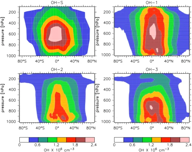
perspec-Fig. 1. The annual zonal mean OH fields based on the four distributions considered here: (a) S (Spivakovsky et al., 2000); (b) OH-1 (Lawrence, OH-1996); (c) OH-2 (Lawrence et al., OH-1999); and (d) OH-3 (von Kuhlmann, 200OH-1). The zonal mean values are computed by weighting every grid cell around a latitude band evenly, which is default for our plotting programs, and presumably for most others. Note, however, that the same arguments discussed in the text apply here: different plots could be produced by computing the zonal OH levels differently, e.g., weighting by the reaction with CH4.

tive of understanding what the global mean OH concentra-tion tells us about the atmospheric oxidizing efficiency with respect to important trace gases, in particular CH4, as well

as CH3CCl3, and how we can best go about comparing OH

levels with this in mind. To do so, we consider [OH]GM

based on four different 3D OH distributions, using several of the various weightings and domains encountered in Ta-ble 1. The four OH distributions chosen for this study are described in the next section; they can be considered rep-resentative of the range of characteristic distributions found in the recent literature. In Sect. 3, we discuss the various techniques used to compute [OH]GM, and the physical

inter-pretation of each of these, in particular their relationship to trace gas lifetimes. Section 4 considers the influence of dif-ferent weighting factors on [OH]GMvalues computed for the

four distributions; Section 5 considers the same for different domains. Sections 6 and 7 examine the regional distribution of CH4and CH3CCl3oxidation in the troposphere, and how

this can be used to help choose a set of subdomains

appro-priate for future comparisons of OH distributions. Section 8 gives our conclusions and recommendations for future stud-ies.

2 OH fields description

We examine [OH]GM using four different global OH

distri-butions. The first one, OH-S, is from the empirical analysis of Spivakovsky et al. (2000), which gives the OH distribu-tion on an 8◦ × 10◦ _{grid in pressure intervals of 100 hPa.}

Their OH levels are computed based on a photochemical box model combined with observed distributions of the main pa-rameters influencing local OH, e.g., O3, H2O, CO, NOx,

hydrocarbons, and solar radiation. The other three global OH distributions used here, OH-1, OH-2, and OH-3, were computed using the global 3D chemistry-transport model MATCH (Model of Atmospheric Transport and Chemistry; Rasch et al. (1997), in its extended configuration

MATCH-MPIC (Max-Planck-Institute for Chemistry version), which includes tropospheric chemistry; output from three differ-ent versions are used here (OH-1 is from MATCH-MPIC 1.2, Lawrence (1996); OH-2 is from MATCH-MPIC 2.0, Lawrence et al. (1999); OH-3 is from MATCH-MPIC 3.0, von Kuhlmann (2001)). All three of these were computed at a relatively high horizontal resolution of about 2 × 2 degrees (T63), with 28 sigma levels between the surface and about 2 hPa. An extensive discussion of the testing of three of these distributions (all but OH-3) using vari-ous tracers such as CH3CCl3 and14CO is given by J¨ockel

(2000). There were numerous differences between the three MATCH-MPIC model versions, in particular the inclusion of non-methane hydrocarbon reactions in computing OH-3 (OH-1 and OH-2 are based on CH4-only chemistry), along

with other major modifications, such as the advection and convection schemes, several emissions fields, and a few key reaction rates, resulting in rather different OH fields (see Lawrence et al. (1999) and von Kuhlmann (2001) for more details).

The annual zonal mean OH levels based on these four dis-tributions are shown in Fig. 1; these and all values discussed here are day and night (24-hour) means, rather than daytime-only means (OH concentrations are very low at night com-pared to day). OH-S is largely hemispherically symmetric, while OH-1, OH-2, and OH-3 have notably more OH in the northern hemisphere. OH-S, OH-1, and OH-3 have the high-est zonal mean OH levels in the tropical mid-troposphere, peaking at about 2.3 × 106molec/cm3in both, at a somewhat higher altitude (600 hPa) in S and 1 than in OH-3 (700 hPa). The OH-2 distribution has a maximum much closer to the surface, and the peak value is lower, around 1.8

× 106_molec/cm3_{. The OH-2 distribution resembles another}

recent study focused on global OH (Krol et al., 1998), while some other models (e.g. Crutzen and Zimmermann, 1991; Wang et al., 1998) compute OH distributions which more closely resemble the OH-S distribution. Although we focus mainly on vertical differences here, there are also important horizontal differences; in particular, OH is depleted over the forested tropical continents in the OH-3 and OH-S distribu-tions, due to the influence of isoprene and other NMHCs on OH in source regions, in contrast to OH-1 and OH-2 (which do not include the effects of NMHCs). These four distribu-tions are used in this study in an effort to represent much of the range of recent estimates of the global OH distribution.

3 Computing the global mean OH concentration

[OH]GM is generally computed from a 2D or 3D OH

distri-bution by applying some type of weighting factor, W:

[OH]GM =

Σ(W · [OH])

ΣW , (1)

where the summation is over all grid cells in a chosen region (e.g., the troposphere). The weighting factor W can take on

different forms. Often either the air mass or the volume are used. The volume-weighted variant (hereafter ([OH]GM(V))

is the literal interpretation of a global mean concentration: all OH molecules spread over the total volume of the tro-posphere. We therefore assume it is likely that some of the studies in Table 1 which did not state the weighting that was used were adopting this literal definition, and thus considered it to be superfluous to specify how [OH]GM was computed.

It is difficult, however, to assign a physical meaning to this quantity in terms of other relevant atmospheric parameters. The airmass-weighted value (hereafter [OH]GM(M)) can be

considered as indicative of the oxidizing efficiency (or life-time) for a uniformly-distributed gas with no temperature or pressure dependence in its reaction with OH (see Equations 2–5 below).

Alternatively, W can be chosen to provide information about the lifetime of a given gas X, in which case the global mean OH concentration (hereafter [OH]GM(X)) is

computed using:

W = kX(T, P ) · MX (2)

where kX is the reaction rate of OH with the gas X,

usu-ally temperature and/or pressure dependent, and MX is the

mass of the gas in a grid cell. X is generally chosen to be a long-lived gas which primarily reacts with OH, in par-ticular CH4 and CH3CCl3. It is occasionally assumed that

the distribution of some long-lived gases such as CH4 and

CH3CCl3 can be treated as uniformly distributed (e.g.

Spi-vakovsky et al., 2000), so that an alternative weighting would be W = kX(T, P ) · Mair, where Mair is the air mass. For

the cases considered here, this assumption is generally very good, and leads to <1% error in the annual mean [OH]GM

values (<5% for monthly values), compared to using MXin

Eq. 2.

In this study, we consider [OH]GM for four

dis-tinct weightings: air mass ([OH]GM(M)); volume

([OH]GM(V)); and the reaction rates with CH4 and

CH3CCl3 ([OH]GM(CH4) and [OH]GM(MCF),

respec-tively; Eq. 2). For the temperature, air mass, and tracer mass fields (CH4 and CH3CCl3) which are needed for

these calculations, we employed the distributions from MATCH-MPIC version 2.0 (for information about the computation of CH4, see Lawrence et al. (1999); for details

about CH3CCl3 emissions, which are the same as in Krol

et al. (1998), and about its sinks, see J¨ockel (2000)); note that we also tested using the fields from an earlier model version (MATCH-MPIC 1.2), and obtained essentially the same results.

As discussed in the introduction, we define the atmo-spheric oxidizing efficiency with respect to a given gas X to be the inverse of the lifetime (τ (X)) of that gas

OEX=

1

Fig. 2. Depictions of the relationships between different ways of computing the tropospheric [OH]GM: (a) [OH]GM values for the

four distributions and four weightings discussed in the text; (b) ratio of [OH]GMvalues for three weightings versus [OH]GM(CH4).

where the lifetime is defined as:

τ (X) = ΣMX Σ(kX· [OH] · MX)

(4) Combining this with equations (1) and (2) for the reaction rate weighted mean OH ([OH]GM(X)) yields:

τ (X) = α · ([OH]GM(X))−1 (5)

where

α = ΣMX Σ(kX· MX)

(6) Thus, for a well-mixed gas, τ (X) and [OH]GM(X) are

in-versely related by the coefficient α, whose value generally depends only on the temperature distribution in the atmo-sphere, the temperature dependence of the reaction, and the domain over which the summation is applied. For the CH4

and CH3CCl3 distributions and reaction rates used here,

integrated over the climatological troposphere domain de-fined below (Eq. 7), α (in yr·molec/cm3) is computed to

Table 2. Global annual mean tropospheric OH concentrations (x106 molec/cm3_{) for different OH distributions and weightings}

Weighting Factor OH-S OH-1 OH-2 OH-3

Air Mass 1.14 1.26 0.88 0.95

Air Volume 1.10 1.28 0.82 0.87 CH4Reaction 1.32 1.39 1.06 1.19

CH3CCl3Reaction 1.29 1.38 1.04 1.16

be 10.86 and 6.41, respectively. The same values (within roundoff) are computed assuming the gases are uniformly distributed. However, integrating over different domains re-sults in considerably different values: below 300 hPa yields 9.54 and 5.71, below 200 hPa yields 10.47 and 6.20, and be-low 100 hPa yields 11.48 and 6.69. This is due to two fac-tors. First, the [OH]GM(CH4) and [OH]GM(MCF) values

do not change much for different vertical domains, since the amount which reacts with CH4and CH3CCl3 in the upper

troposphere is minimal (see Sect. 6), so that the UT is only weighted weakly. On the other hand, the lifetime is strongly dependent on the vertical extent over which it is computed; for example, extending the upper bound to a higher altitude does not add much to the total loss (in Tg/yr), but it does add to the tracer mass (in Tg). Thus, since in Eq. 5 [OH]GM(X)

is relatively constant with altitude, whereas τ (X) varies no-tably, α must also vary strongly with the extent of the tropo-spheric domain.

Table 3. Global annual mean tropospheric lifetimes (years) for CH4

and CH3CCl3

Gas OH-S OH-1 OH-2 OH-3

CH4 8.23 7.79 10.25 9.12

CH3CCl3 4.95 4.66 6.16 5.50

4 Influence of the weighting factor on [OH]GM

In this section the differences in [OH]GMvalues due to using

different weightings will be discussed. [OH]GMbased on the

OH distributions and weightings discussed above are given in Table 2 and Fig. 2. The implied lifetimes for CH4 and

CH3CCl3are also listed (Table 3).

Monthly mean fields (OH, CH4, etc.) were used in these

computations. Since temperatures are usually higher during the daytime, when OH concentrations are highest, one might expect higher [OH]GMvalues if hourly data were to be used

in Equations 1 and 2 instead of monthly means. To test this effect we performed a 1-month run for March conditions at a reduced model resolution (T21, about 5.6 degrees in latitude

and longitude). When we use the hourly values in Eqs. 1 and 2 and then average to get the value of [OH]GM for the

month, we get less than a 1% difference from when we in-stead simply use the 1-month mean values of [OH] and T to compute [OH]GM. Thus, we can confidently employ the

monthly [OH]GM values based on monthly mean [OH] and

T fields, and then average these to yield annual means. Only the annual mean results are discussed here; values for indi-vidual months lead to the same conclusions as the annual means.

In this section, results are only considered for the domain below a climatological tropopause, defined as

p = 300 − 215(cos(φ))2 (7)

where p is the pressure in hPa, and φ is the latitude (see J¨ockel (2000) for further discussion of this tropopause def-inition); differences due to the definition of the tropospheric domain are considered in the next section.

The spread ((maximum-minimum)/average) in [OH]GM

calculated using the different weightings is about 18% for S, 10% for 1, 25% for 2, and 31% for OH-3, comparable to or larger than the uncertainty ranges in [OH]GM stated by Spivakovsky et al. (2000), Krol et al.

(1998), and Prinn et al. (1995, 2001). The results indicate that weighting by the reaction with CH4or CH3CCl3always

yields the highest values for [OH]GM. This is due to the

strong temperature dependence of these reactions, so that the tropics and the mid to lower troposphere, where OH con-centrations are highest (Fig. 1), are weighted most strongly. [OH]GM(M) and [OH]GM(V) are generally closer to each

other than to [OH]GM(CH4) and [OH]GM(MCF), though the

relationship between the parameters is rather variable. The differences are smallest for OH-1, which is most evenly dis-tributed in the vertical throughout the troposphere (Fig. 1). The other distributions, with OH falling off sharply in the tropical upper troposphere, show larger differences between the four different [OH]GM values, especially OH-2, which

is weighted most strongly towards the surface, and OH-3, which falls off at lower altitudes in the tropics than the other distributions.

Figure 2b shows the ratio of [OH]GM(M), [OH]GM(V)

and [OH]GM(MCF) to [OH]GM(CH4) for each of the four

OH distributions. Recall that [OH]GM(CH4) is directly

re-lated to the inverse of τ (CH4) (Eq. 5), and thus to OECH4.

In order for any of the other three parameters to also serve as a good indicator of the oxidizing efficiency with respect to CH4 which is applicable to any “typical” OH

distri-bution, then they should have a consistent relationship to [OH]GM(CH4), i.e., they should yield approximately

hor-izontal lines on Fig. 2b. While [OH]GM(MCF)

essen-tially fulfills this criterion, the two “generic” parameters [OH]GM(M) and [OH]GM(V) clearly do not. The ratio

be-tween [OH]GM(M) and [OH]GM(CH4) differs by >10%,

while for [OH]GM(V) the ratio varies by >20%.

Although the principle behind the result in Fig. 2b is clear, since the relationship between OH amounts and OECH4

de-pends on the geographical distribution of OH, to date it has not been made clear how much the relationship between [OH]GM(M), [OH]GM(V) and [OH]GM(CH4) (or τ (CH4))

should actually vary for current estimates of the OH distri-bution. Based on Fig. 2b we conclude that [OH]GM(M) and

[OH]GM(V) are not very good indicators of the atmospheric

oxidizing efficiency with respect to long-lived gases with strong temperature dependences such as CH4and CH3CCl3,

at least not on a global basis. However, when the atmosphere is broken down into smaller domains, over which the tem-perature and OH concentration do not vary as much, then the ability of the airmass- and volume- weighted regional mean OH values to represent the regional OECH4 (or OEM CF)

values improves considerably, as discussed in Section 7.

5 Influence of the tropospheric domain on [OH]GM

In this section, the differences in [OH]GM computed over

four different domains are considered: (1) the region below the climatological tropopause defined in Eq. 7, (2) the re-gion below 100 hPa, (3) the rere-gion below 200 hPa, and (4) the region below 300 hPa. The first three represent the ex-tremes of what is encountered in Table 1, while the latter is included because it is purely tropospheric, and contains the region where atmospheric gases like CH4and CH3CCl3are

mainly oxidized (discussed in the next section).

The ratios of [OH]GM(M), [OH]GM(V), τ (CH4), and

τ (CH3CCl3) for the latter three domains versus the values

for the climatological troposphere are depicted in Fig. 3, which shows that the volume-weighted OH values are par-ticularly strongly affected by the chosen domain, varying by 20% or more for the region below 100 hPa versus that be-low 300 hPa. The lifetimes of CH4 and CH3CCl3 are

al-most as strongly affected, also varying by nearly 20%, while [OH]GM(M) varies by about 10%. Restricting this to only

the domains encountered in Table 1 (i.e., all but Fig. 3c), the differences are about 10% for [OH]GM(V), τ (CH4), and

τ (CH3CCl3), and about 5% for [OH]GM(M). The OH

distri-bution which shows the least sensitivity to domain is OH-1, due to the relatively high tropical OH values extending ver-tically to about the 100 hPa level. In contrast, the variation in τ (CH4) and τ (CH3CCl3) is similar for all four OH

distri-butions, since the amount of tracer which is oxidized in the upper troposphere mainly depends on the rapidly falling tem-perature, rather than the OH values. On a similar note, the ra-tios of values for [OH]GM(CH4) and [OH]GM(MCF) are not

shown in the figure, since they are all in the range 0.99–1.02. The reason for the weak dependence of these quantities on the chosen tropospheric domain, as discussed previously, is that very little oxidation of CH4and CH3CCl3occurs in the

upper troposphere, and thus the values in the region above 300 hPa are hardly weighted in computing [OH]GM(CH4)

Fig. 3. The ratios of [OH]GM(M), [OH]GM(V), τ (CH4), and

τ (CH3CCl3) for (a) the domain below 100 hPa, (b) the domain

be-low 200 hPa, and (c) the domain bebe-low 300 hPa, versus the values for the climatological troposphere (Eq. 7).

and [OH]GM(MCF). This issue is considered further in the

next section.

6 The distribution of CH4 and CH3CCl3 oxidation in

the troposphere

It has been well established in previous studies that CH4

oxi-dation is weighted towards the tropics (e.g. Crutzen and Zim-mermann, 1991; Crutzen et al., 1999); in addition, it is known that the lifetime of CH4increases significantly with altitude

(e.g. Krol and van Weele, 1997). Because the vertical distri-bution of CH4oxidation plays an important role in the

rela-tionship between [OH]GMand OECH4, as discussed above,

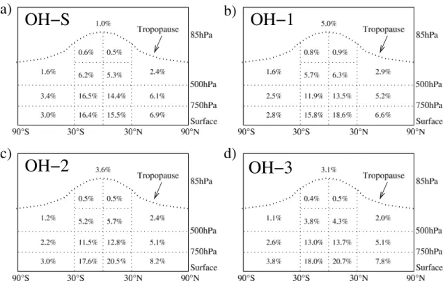
we examine this in more detail here. In Fig. 4 we show the breakdown of the percentage of oxidation of CH4which

oc-curs in selected subdomains of the atmosphere, where the breakdown is computed based on the OH distributions con-sidered here. Figure 5 gives an overall impression of this breakdown as the average of the values for all four OH dis-tributions in Fig. 4 taken over larger subdomains, along with the same summary information for CH3CCl3.

The values in Fig. 4 are a reflection of the OH distributions in Fig. 1 and the temperature distribution in the atmosphere (along with the slight asymmetry in CH4, with ∼10% more

in the NH). We find that in the extratropics (30◦–90◦), more is oxidized in the NH than in the SH in all four of the distribu-tions. The OH-S distribution yields an opposite asymmetry in the tropics, so that on the whole the amount of CH4

oxida-tion (and the OH amounts) based on OH-S is roughly hemi-spherically symmetric; however, this results from the balance between the opposing asymmetries in the tropics and extra-tropics. The MATCH OH distributions, on the other hand, favor the NH in both the tropics and the extratropics. The north-south asymmetry has been discussed in several studies; often model results, such as those shown here, are in con-tradiction with observational evidence (e.g. Brenninkmeijer et al., 1992; Montzka et al., 2000). The reasons for this are currently unclear; one possible contributing factor is that the OH estimates based on CH3CCl3observations are influenced

by the fact that the ITCZ, which separates the meteorologi-cal NH and SH, lies on average a few degrees north of the equator (Montzka et al., 2000).

The summary in Fig. 5 shows the dominance of the trop-ical lower troposphere in the overall oxidation of CH4 and

CH3CCl3, where on average >60% of the total oxidation

occurs. The tropical mid troposphere, and the extratropical lower tropospheric regions, particularly in the NH, play sec-ondary roles. The upper troposphere and stratosphere com-bined are responsible for <10% of the total oxidation of these gases, and the region above 250 hPa accounts for <5% of the total. This indicates that the focus on comparing mean OH concentrations, to the extent that these should be indicative of OECH4 or OEM CF, should be on the lower and mid

Fig. 4. The percentages of CH4which are oxidized in various subdomains of the atmosphere based on four different OH distributions: (a)

OH-S; (b) OH-1; (c) OH-2; (d) OH-3. The horizontal lines in the tropical upper tropospheric regions are at 250 hPa.

Fig. 5. The percentages of (a) CH4 and (b) CH3CCl3 which are

oxidized in various subdomains of the atmosphere based on the av-erage of the four OH distributions (OH-S, OH-1, OH-2, and OH-3). Numbers may not add up to exactly 100% due to roundoff.

7 Atmospheric subdomains for comparing OH distribu-tions

Figure 4 can be used to help devise a strategy for compar-ing modeled OH distributions. This should be a balance be-tween: (1) sufficient information to really judge whether OH distributions are similar, at least in terms of their role in de-termining the atmospheric oxidizing efficiency; (2) manage-ability of the amount of numbers to compare, and (3) appli-cability to various model settings. In this regard, a generic parameter (airmass or volume weighted [OH]), rather than one tied to a specific gas (e.g., CH4), would be desirable,

since it would make the comparison less dependent on model parameters such as the temperature and trace gas distribu-tions. However, as found above, this does not work well on a global basis, so that a breakdown into atmospheric subdo-mains needs to be considered.

We propose a breakdown in the horizontal at 30◦S, 0◦, and 30◦N, following Prinn et al. (1995, 2001), and vertical divi-sions at 750, 500, and 250 hPa, which gives approximately equal masses in each of the 12 atmospheric compartments below 250 hPa (Krol, 2001). The importance of the vertical division at 750 hPa can be seen by comparing the OH-S re-sults with the other rere-sults in Fig. 4. While the OH-1, OH-2, and OH-3 distributions have about 50% more CH4oxidation

in the lowermost layer (surface–750 hPa) than in the middle layer (750–500 hPa), the OH-S distribution results in nearly

even amounts of oxidation in the two vertical domains. In this case, it would be clearly possible for the distributions to have similar airmass- or volume-weighted mean OH concen-trations in the larger region between the surface and 500 hPa, but very different oxidizing efficiencies with respect to CH4.

We do not include the region above 250 hPa, since it was shown in the previous section to be responsible for less than 5% of the oxidation of gases such as CH4with strong

temper-ature dependences in their reaction with OH. Since the lowest level of most contemporary models is not fixed at 1000 hPa, but instead has a variable surface pressure, the airmass in the regions from the surface to 750 hPa will deviate slightly from the 3.3 ×1020kg in each of the other regions; from south to north, for our model data we compute masses of 3.1, 3.4, 3.3, and 3.0 ×1020kg for these four boxes.

For each of the 12 subdomains suggested here, the rela-tionship between [OH]RM(M) and [OH]RM(CH4), where

the subscript RM indicates the regional mean, is relatively constant; the same applies to τ (CH4). In comparison to the

spread of >10% seen in Fig. 2b, the mean spread in the ra-tio of [OH]RM(M)/[OH]RM(CH4) for the four OH

distribu-tions broken down into each of these 12 regions is 3.1%, with a standard deviation of 1.0%. The spread in the vol-ume weighted regional means ([OH]RM(V)/[OH]RM(CH4))

is somewhat worse, averaging 4.6±1.6%. Thus, the [OH]RM(M) (and to a lesser extent [OH]RM(V)) values

bro-ken down into these regions can be considered as representa-tive of OECH4in each region, and should provide an

appro-priate test of modeled OH distributions.

8 Conclusions and recommendations

What does the global mean OH concentration tell us about modeled OH distributions and amounts and about the ox-idizing efficiency of the atmosphere? We have shown in this study that the answer to this depends critically on the weighting which is used to compute this value, as well as the domain over which it is integrated. We found that dif-ferences in [OH]GM, the global mean OH concentration, can

be as large as 30% due to employing different weightings which have historically been used, and >10% for different domains. These numbers are comparable to the stated un-certainty in [OH]GM (e.g. Prinn et al., 2001; Spivakovsky

et al., 2000; Krol et al., 1998). They are also significant in light of the consideration that all but a few of the values in Tables 1 and 2 lie within about 50% of each other (range 0.75–1.25 molec/cm3_{). Since widely varying studies tend}

to give [OH]GM values which lie within this relatively

lim-ited range, a meaningful comparison between [OH]GMfrom

different studies can only be done with similarly-computed values. Otherwise it is difficult to determine whether any agreement in [OH]GM from different studies is coincidental

or real. The same principle also applies to trends in [OH]GM

values when they are computed using different weightings.

For example, consider the scenario in which the total number of OH molecules increases by a certain amount (say 1%/yr). This would lead to the same trend in the volume-weighted [OH]GM value, regardless of whether the increase occurs

in the upper troposphere or near the surface. In contrast, the same increase would cause a larger trend in airmass-weighted or CH4-reaction-weighted [OH]GM if it occurred

near the surface than if it occurred higher up. However, it is important to note that trends are not always computed based on year-to-year differences in modeled annual mean OH distributions; these arguments will not apply, for in-stance, when the OH trend is computed by scaling to deter-mine the CH3CCl3loss rate (Krol, 2001).

In this study we have focused on how to compare OH dis-tributions in light of their ability to serve as indicators of

OEX, the global oxidizing efficiency with respect to a given

gas X, which we define as the inverse of τ (X), the lifetime of X. We showed that [OH]GM is directly proportional to

OEX (i.e., inversely proportional to τ (X)) only when it is

weighted by the reaction with X ([OH]GM(X)), in which

case the proportionality coefficient depends only on the do-main of integration, the reaction rate coefficient, and the tem-perature distribution. In contrast to this, on a global basis nei-ther the airmass-weighted nor the volume-weighted [OH]GM

values are very good indicators of the atmospheric oxidizing efficiency with respect to important long-lived gases such as CH4with strong temperature dependences in their reaction

with OH, since they are not sensitive to the regions where temperatures are highest, and thus where oxidation reactions are fastest. However, when the atmosphere is broken down into smaller domains, over which [OH] and the temperature vary less significantly, then it was shown that the airmass-weighted regional mean OH concentration, [OH]RM(M), can

also serve as a good indicator of the regional oxidizing effi-ciency for such gases.

The findings in this study lead us to the following recom-mendations for future studies:

1. Global mean OH would best be given in two forms: weighted with the reaction with CH4 (Eq. 2), and

weighted with the air mass; the former provides a direct indication of the atmospheric oxidizing efficiency with respect to the most important greenhouse gas which is mainly removed by reaction with OH, and is rather in-sensitive to differences in the vertical extent of the tro-pospheric domain used in its computation; the latter is indicative of OEX for a gas with no temperature

de-pendence in its reaction with OH, and is more sensitive to the averaging domain; we suggest using the domain defined by the climatological tropopause given in Eq 7; the combination of these two values helps give an initial screening for when two OH distributions are different, even if their global mean values for one of these weight-ings is coincidentally similar;

2. Serious evaluations of modeled OH distributions should break down the OH distribution into regional mean airmass-weighted values ([OH]RM(M)) in tropospheric

subdomains, in particular the 12 which have been dis-cussed here. For future comparisons, the [OH]RM(M)

values in each of these 12 subdomains for the four OH distributions considered here are given in Table 4. In addition, the tropospheric lifetimes of CH4(τ (CH4)) and

CH3CCl3 (τ (MCF)) can also be provided as additional

pa-rameters related to the OH distribution since they can be compared directly with independent estimates of their val-ues (e.g., from analyses of source strengths, atmospheric bur-dens, and growth or decline rates); again, we recommend using the domain defined by the climatological tropopause given in Eq. 7.

The second recommendation is clearly a difficult one to adopt on a widespread basis, since it is generally desirable to have a single number, where possible, which indicates model performance. However, we feel it is critical that the distribu-tion of OH be taken into consideradistribu-tion in this or a similar way in future studies. Concluding that a model simulation of OH is “reasonable” because the global mean OH concentra-tion is in good agreement with that from another study can be misleading, since two OH distributions can readily have the same [OH]GM values computed using different

weight-ings, but very different distributions (e.g., one more concen-trated towards the surface than the other), which could re-sult in different oxidizing efficiencies. Although we do not wish to single out any particular studies here, we have found several instances in the literature in which such comparisons of differently-computed [OH]GMvalues have been made (in

some cases apparently inadvertently, due to misinterpretation of other studies where the weighting which was used was un-clear).

Our proposal for a single number which indicates the de-gree of ade-greement between various OH fields, both in terms of their amounts and their distributions, is the RMS devi-ation between [OH]RM(M) for two distributions in the 12

subdomains depicted in Table 4. For the MATCH-MPIC OH distributions relative to the OH-S distribution, these values are (in 106molec/cm3): 0.21 (OH-1), 0.37 (OH-2), and 0.33 (OH-3). When considered in light of the global mean val-ues of order 1×106 molec/cm3, these RMS differences are relatively high; they are nearly twice as large as the mean deviations based on the global values in Table 2 (0.12, 0.26, and 0.17, respectively). Thus, since our proposed approach is sensitive to both the OH amounts and its distribution (par-ticularly the differences in the tropical vertical distributions seen in Fig. 1), it provides much more information than sim-ply comparing global means does about the degree to which various OH distributions agree or disagree.

We offer these recommendations as a starting point for dis-cussion by the community, and are open to suggestions of alternate details regarding the recommendations or alternate

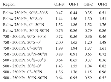
Table 4. Regional annual mean airmass-weighted OH concentra-tions (x106molec/cm3) for different OH distributions in the recom-mended subdomains

Region OH-S OH-1 OH-2 OH-2

Below 750 hPa, 90◦S–30◦S 0.47 0.44 0.35 0.51 Below 750 hPa, 30◦S–0◦ 1.44 1.56 1.30 1.51 Below 750 hPa, 0◦–30◦N 1.52 1.86 1.52 1.76 Below 750 hPa, 30◦N–90◦N 0.76 0.86 0.79 0.86 750 - 500 hPa, 90◦S–30◦S 0.72 0.56 0.36 0.46 750 - 500 hPa, 30◦S–0◦ 2.00 1.65 1.20 1.48 750 - 500 hPa, 0◦–30◦N 1.99 1.94 1.37 1.61 750 - 500 hPa, 30◦N–90◦N 0.88 0.91 0.65 0.72 500 - 250 hPa, 90◦S–30◦S 0.64 0.65 0.37 0.36 500 - 250 hPa, 30◦S–0◦ 1.43 1.55 1.04 0.82 500 - 250 hPa, 0◦–30◦N 1.36 1.76 1.15 0.96 500 - 250 hPa, 30◦N–90◦N 0.64 0.95 0.59 0.52

approaches to those proposed here, as long a standard is de-fined by the community and adhered to so that values from different studies can be directly compared. There are a num-ber of related issues which are in particular need of further consideration. First, we have focused on the oxidizing effi-ciency with respect to CH4and CH3CCl3in this study, since

they are important, long-lived gases with relatively uniform distributions in the troposphere. It is formally possible to define an oxidizing efficiency with respect to shorter-lived gases such as CO; however, this would be more difficult to interpret and particularly to compare between different stud-ies, since the oxidizing efficiencies for such gases strongly depend on both the OH distribution and the distribution of the gas in question. This issue could be considered further in future studies. Another point which will need to be consid-ered is how to handle updates in the rate coefficients of OH with CH4and other gases, which affects the lifetime and the

[OH]GM(X) values computed based on a given OH

distribu-tion. Finally, we recommend that the atmospheric research community develop clear, broadly accepted definitions of the terms “oxidizing efficiency”, “oxidizing power”, “oxi-dizing capability”, and “oxi“oxi-dizing capacity”; various defini-tions have been used in the past (e.g. Thompson, 1992), and a working definition for the oxidizing efficiency has been pro-posed here.

Acknowledgements. We appreciate useful comments from Jos

Lelieveld, Paul Crutzen, Jonathan Williams, Ulrich P¨oschl, and Benedikt Steil. The thoughtful reviews of Maarten Krol and an anonymous referee helped to strengthen this manuscript. This work was supported by funding from the German Ministry of Education and Research (BMBF), project 07-ATC-02.

References

Atkinson, R.: Atmospheric chemistry of VOCs and NOx, Atmos.

Environ., 34, 2063–2101, 2000.

Berntsen, T. K. and Isaksen, I. S. A.: A global three-dimensional chemical transport model for the troposphere, 1. model descrip-tion and CO and ozone results, J. Geophys. Res., 102, 21 239– 21 280, 1997.

Bolin, B. and Rodhe, H.: A note on the concepts of age distribution and transit time in natural reservoirs, Tellus, 25, 58–62, 1973. Brasseur, G. P., Orlando, J. J., and Tyndall, G. S.: Atmospheric

Chemistry and Global Change, Oxford University Press, New York, 1999.

Brenninkmeijer, C., Manning, M., Lowe, D., Wallace, G., Sparks, R., and Volz-Thomas, A.: Interhemispheric asymmetry in OH abundance inferred from measurements of atmospheric14CO, Nature, 356, 50–52, 1992.

Chameides, W. L. and Walker, J. C. G.: A photochemical theory of tropospheric ozone, J. Geophys. Res., 78, 8751–8760, 1973. Collins, W. J., Stevenson, D. S., Johnson, C. E., and Derwent,

R. G.: Tropospheric ozone in a global-scale three-dimensional lagrangian model and its response to NOxemission controls, J.

Atmos. Chem., 26, 223–274, 1997.

Crutzen, P. and Zimmermann, P. H.: The changing photochemistry of the troposphere, Tellus, 43 AB, 136–151, 1991.

Crutzen, P. J.: Gas-phase nitrogen and methane chemistry in the atmosphere, Report AP-10, University of Stockholm, 1972. Crutzen, P. J.: A discussion of the chemistry of some minor

con-stituents in the stratosphere and troposphere, Pure and Applied Geophysics, 106–108, 1385–1399, 1973.

Crutzen, P. J.: Photochemical reactions initiated by and influencing ozone in unpolluted tropospheric air, Tellus, 16, 47–56, 1974. Crutzen, P. J. and Lawrence, M. G.: The impact of precipitation

scavenging on the transport of trace gases: A 3-dimensional model sensitivity study, J. Atmos. Chem., 37, 81–112, 2000. Crutzen, P. J., Lawrence, M. G., and P¨oschl, U.: On the

back-ground photochemistry of tropospheric ozone, Tellus, 51, 123– 146, 1999.

Derwent, R.: The influence of human activities on the distribution of hydroxyl radicals in the troposphere, Phil. Trans. Roy. Soc. London A, 354, 501–531, 1996.

Hein, R., Crutzen, P. J., and Heimann, M.: An inverse modeling approach to investigate the global atmospheric methane cycle, Global Biogeochem. Cycles, 11, 43–76, 1997.

Hough, A. M.: Development of a two-dimensional global tropo-spheric model: model chemistry, J. Geophys. Res., 96, 7325– 7362, 1991.

Jaegl´e, L., Jacob, D. J., Brune, W. H., and Wennberg, P. O.: Chem-istry of HOxradicals in the upper troposphere, Atmos. Environ.,

35, 469–489, 2001.

J¨ockel, P.: Cosmogenic14CO as a tracer for atmospheric chemistry and transport, Ph.D. thesis, Universit¨at Heidelberg, http://www. ub.uni-heidelberg.de/archiv/1426, 2000.

Karlsdottir, S. and Isaksen, I. S. A.: Changing methane lifetime: Possible cause for reduced growth, Geophys. Res. Lett., 27, 93– 96, 2000.

Kashibhatla, P., Levy II, H., Moxim, W. J., Pandis, S. N., Corbett, J. J., Peterson, M. C., Honrath, R. E., Frost, G. J., Knapp, K., Parrish, D. D., and Ryerson, T. B.: Do emissions from ships have a significant impact on concentrations on nitrogen oxides in the

marine boundary layer?, Geophys. Res. Lett., 27, 2229–2232, 2000.

Kiehl, J., Schneider, T., Rasch, P., Barth, M., and Wong, J.: Radia-tive forcing due to sulfate aerosols from simulations with the na-tional center for atmospheric research community climate model, version 3, J. Geophys. Res., 105, 1441–1457, 2000.

Krol, M.: Interactive Comment on “What does the global mean OH concentration tell us?” by “M. G. Lawrence et al.”, Atmos. Chem. Phys. Discuss., 1, S1–S5, 2001.

Krol, M., van Leeuwen, P. J., and Lelieveld, J.: Global OH trend in-ferred from methyl-chloroform measurements, J. Geophys. Res., 103, 10 697–10 711, 1998.

Krol, M. C. and van Weele, M.: Implications of variations in pho-todissociation rates for global tropospheric chemistry, Atmos. Environ., 31, 1257–1273, 1997.

Lawrence, M. G.: Photochemistry in the Tropical Pacific Tro-posphere: Studies with a Global 3D Chemistry-Meteorology Model, Ph.D. thesis, Georgia Institute of Technology, 1996. Lawrence, M. G. and Crutzen, P. J.: Influence of NOxemissions

from ships on tropospheric photochemistry and climate, Nature, 402, 167–170, 1999.

Lawrence, M. G., Crutzen, P. J., Rasch, P. J., Eaton, B. E., and Mahowald, N. M.: A model for studies of tropospheric photo-chemistry: Description, global distributions, and evaluation, J. Geophys. Res., 104, 26 245–26 277, 1999.

Levy, H.: Normal atmosphere: Large radical and formaldehyde concentrations predicted, Science, 173, 141–143, 1971. Montzka, S. A., Spivakovsky, C. M., Butler, J. H., Elkins, J. W.,

Lock, L. T., and Mondeel, D. J.: New observational constraints for atmospheric hydroxyl on global and hemispheric scales, Sci-ence, 288, 500–503, 2000.

Poisson, N., Kanakidou, M., and Crutzen, P. J.: Impact of non-methane hydrocarbons on tropospheric chemistry and the oxidiz-ing power of the global troposphere: 3-dimensional modelloxidiz-ing results, J. Atmos. Chem., 36, 157–230, 2000.

Prather, M. J. and Spivakovsky, C. M.: Tropospheric OH and the lifetimes of hydrochlorofluorocarbons, J. Geophys. Res., 95, 18 723–18 729, 1990.

Prinn, R. G., Weiss, R. F., Miller, B. R., Huang, J., Alya, F. N., Cunnold, D. M., Fraser, P. J., Hartley, D. E., and Simmonds, P. G.: Atmospheric trends and lifetime of CH3CCl3and global

OH concentrations, Science, 269, 187–190, 1995.

Prinn, R. G., Huang, J., Weiss, R. F., Cunnold, D. M., Fraser, P. J., Simmonds, P. G., McCulloch, A., Harth, C., Salameh, P., O’Doherty, S., Wang, R. J. J., Porter, L., and Miller, B. R.: Evi-dence for substantial variations of atmospheric hydroxyl radicals in the past two decades, Science, 292, 1882–1888, 2001. Rasch, P. J., Mahowald, N. M., and Eaton, B. E.: Representations of

transport, convection and the hydrologic cycle in chemical trans-port models: Implications for the modeling of short lived and soluble species, J. Geophys. Res., 102, 28 127–28 138, 1997. Roelofs, G.-J. and Lelieveld, J.: Tropospheric ozone simulation

with a chemistry-general circulation model: Influence of higher hydrocarbon chemistry, J. Geophys. Res., 105, 22 697–22 712, 2000.

Spivakovsky, C. M., Yevich, R., Logan, J. A., Wofsy, S. C., McEl-roy, M. B., and Prather, M. J.: Tropospheric OH in a three-dimensional chemical tracer model: An assessment based on observations of CH3CCl3, J. Geophys. Res., 95, 18 441–18 471,

Spivakovsky, C. M., Logan, J. A., Montzka, S. A., Balkanski, Y. J., Foreman-Fowler, M., Jones, D. B. A., Horowitz, L. W., Fusco, A. C., Brenninkmeijer, C. A. M., Prather, M. J., Wofsy, S. C., and McElroy, M. B.: Three-dimensional climatological distribution of tropospheric OH: Update and evaluation, J. Geophys. Res., 105, 8931–8980, 2000.

Thompson, A. M.: The oxidizing capacity of the earth’s atmo-sphere: Probable past and future changes, Science, 256, 1157– 1165, 1992.

Von Kuhlmann, R.: Photochemistry of Tropospheric Ozone, its Pre-cursors and the Hydroxyl Radical: A 3D-Modeling Study Con-sidering Non-Methane Hydrocarbons, Ph.D. thesis, Johannes Gutenberg-Universit¨at Mainz, Mainz, Germany, 2001.

Wang, K.-Y., Pyle, J. A., Shallcross, D. E., and Larry, D. J.: Formu-lation and evaluation of IMS, an interactive three-dimensional tropospheric chemical transport model 2. model chemistry and comparison of modelled CH4, CO, and O3 with surface

mea-surements, J. Atmos. Chem., 38, 31–71, 2001.

Wang, Y., Logan, J. A., and Jacob, D. J.: Global simulation of tro-pospheric O3-NOx-hydrocarbon chemistry, 2. model evaluation

and global ozone budget, J. Geophys. Res., 103, 10 727–10 755, 1998.

Yin, F., Grosjean, D., and Seinfeld, J.: Photooxidation of dimethyl sulfide and dimethyl disulfide .1. mechanism development, J. At-mos. Chem., 11, 309–364, 1990.