HAL Id: inria-00413351
https://hal.inria.fr/inria-00413351
Submitted on 3 Sep 2009
HAL is a multi-disciplinary open access
archive for the deposit and dissemination of
sci-entific research documents, whether they are
pub-lished or not. The documents may come from
teaching and research institutions in France or
abroad, or from public or private research centers.
L’archive ouverte pluridisciplinaire HAL, est
destinée au dépôt et à la diffusion de documents
scientifiques de niveau recherche, publiés ou non,
émanant des établissements d’enseignement et de
recherche français ou étrangers, des laboratoires
publics ou privés.
Fast Delaunay Triangulation for Converging Point
Relocation Sequences
Pedro Machado Manhães de Castro, Olivier Devillers
To cite this version:
Pedro Machado Manhães de Castro, Olivier Devillers. Fast Delaunay Triangulation for
Converg-ing Point Relocation Sequences. European Workshop on Computational Geometry, 2009, Bruxelles,
Belgium. �inria-00413351�
Fast Delaunay Triangulation for Converging Point Relocation
Sequences
Pedro Machado Manh˜aes de Castro* Olivier Devillers∗
Abstract
This paper considers the problem of updating efficiently a Delaunay triangulation when vertices are moving under small perturbations. Its main contribution is a set of algo-rithms based on the concept of vertex tolerance. Experi-ments show that it is able to outperform the naive rebuild-ing algorithm in certain conditions. For instance, when points, in two dimensions, are relocated by Lloyd’s iter-ations, our algorithm performs several times faster than rebuilding.
1 Introduction
Delaunay triangulation of a set of points is one of the most famous data structures produced by computational geom-etry. Two main reasons explain this success: –1– compu-tational geometers eventually produce efficient algorithms to compute it, and –2– it has many practical uses such as meshing for finite elements methods or surface reconstruc-tion from point clouds.
For several applications the data are moving and thus the triangulation evolves with time. It arises for example when meshing deformable objects [4], or in some algo-rithms relocating the points by variational methods [1].
We first recall that the Delaunay triangulation DT(S) of a set S of n points inRd is a simplicial complex such that no point in S is inside the circumsphere of any simplex in DT(S). Several algorithms to compute the Delaunay triangulation are available in the literature. Many of them work in the static setting, where the points are fixed and known in advance. There are also a variety of so-called dynamic algorithms [5], in which the points are fixed but not known in advance and thus the triangulation is main-tained under point insertions or deletions. If some of the points move continuously inRdand we want to keep track of the modifications of the triangulation, we are dealing with kinetic algorithms [8]. Finally, an important variation is when the points move but we are only interested in the triangulation at some discrete times, we call that context timestamps relocation.
When we are in the context of timestamps relocation, a simple and efficient method to consider is the follow-ing: for each timestamp we simply recompute the
Delau-*Email: [email protected]. INRIA, BP93, 06902
Sophia-Antipolis, France, www.inria.fr/sophia/members/First.Lastname. The authors wish to thank the ANR Triangles, contract number
ANR-07-BLAN-0319, and region PACA for their support.
nay triangulation of the set S(t) at timestamp ti. We call this algorithm rebuilding. Note that this algorithm does not take any previous work into account, thus for times-tamp ti it does not benefit from any possible correlation between S(tj) and S(ti), with tj < ti. If points are well-distributed, it could achieve an O(kn log(n)) computation time, where n is the number of vertices on the triangula-tion and k is the number of distinct timestamps.
Although the rebuilding algorithm is naive and has a poor theoretical complexity, it stands for an algorithm hard to outperform when most of the points move, as observed in previous work [8]. In this paper, we propose to com-pute for each point a safety zone where the point can move without changing its connectivity in the triangulation. Sev-eral experiments conducted on synthetic and practical data show added value of the method, in particular for mesh smoothing [2] where the points are converging to a final position.
2 Safe regions
Given any certificate C : Am → {−1, 0, 1} acting on a
m-tuple of points ζ = (z1, z2, . . . , zm) ∈ Am, whereA is the space where the input lies in, we define the tolerance of C with respect to ζ, namely ǫC(ζ) or simply ǫ(ζ) when there is no ambiguity, the largest displacement applicable to z in ζ without invalidating C. Hereafter, a certificate is valid when it is positive. Then, more precisely, the toler-ance can be stated as follows:
ǫC(ζ) = inf ζ′ C(ζ′)≤0 distH(ζ, ζ ′ ), (1)
where distH(ζ, ζ′) is the Hausdorff distance between two finite sets of points.
By abuse of notation, z∈ ζ means that z is one of the points of ζ. LetX be a finite set of m-tuples of points in Am, then the tolerance of an element e∈ A with respect to a given certificate C andX , namely ǫC,X(e) or simply
ǫ(e) when there is no ambiguity, can be defined as follows: ǫC,X(e) = inf
ζ∋e
ζ∈X
ǫC(ζ). (2)
The tolerance involved in a Delaunay triangulation is the tolerance of the empty-sphere certificate acting on any bi-cell of a Delaunay triangulation. From Equation 1, it corresponds to the size of the smallest perturbation the bi-cell’s vertices could undergo so as to become cospherical.
This is equivalent to compute the hypersphere that min-imizes the maximum distance to the d+ 2 vertices, or to compute half the width of the d-annulus of minimum width containing the vertices.
LetT be a triangulation lying in Rd andB a bi-cell in
T . The interior facet of B is the common facet of the two cells ofB. The opposing vertices of B are the remaining two vertices that do not belong to its interior facet. Two bi-cellsB, B′are neighbors if they share a cell. If the interior facet and opposing vertices of B are respectively inside and outside (or on) a common hypersphereS, we say that B verifies the safety condition. We call B a safe bi-cell andS its delimiter. If a vertex z belongs to the interior facet of B, then the safe region of z with respect to B is the region inside the delimiter. Otherwise, the safe region of z with respect toB is the region outside the delimiter. The intersection of the safe regions of z with respect to each one of its adjacent bi-cells is the safe region of z. Finally, if all the bi-cells ofT are safe bi-cells, then we callT a safe triangulation. When a triangulation is a safe triangulation, we say that it verifies the safety condition.
It is clear that a safe triangulation is equivalent to a De-launay triangulation, since:
• Each delimiter can be shrunk in such a way that it touches the vertices of the interior facet, and thus defining an empty-sphere passing through the interior facet of its bi-cell.
• The empty-sphere property of Delaunay triangulation facets defines itself an empty-sphere passing through the interior facets of the bi-cells. Those empty-spheres are delimiters.
Proposition 1 Given a Delaunay triangulation T, if its vertices move arbitrarily yet inside their safe regions, then
T remains Delaunay.
It is a direct consequence of the equivalence between safe and Delaunay triangulations, since if the vertices remains inside their safe regions, thenT remains a safe triangula-tion, and hence a Delaunay triangulation.
Among all possible delimiters of a bi-cell, we define the standard delimiter as the median hypersphere of the d-annulus with the inner-hypersphere passing through the interior facet and the outer-hypersphere passing through the opposing vertices. Both median hypersphere and d-annulus are unique. We call the d-d-annulus, the generator of the standard delimiter.
LetD(B) be the delimiter of a given bi-cell B. Then, for a given vertex z∈ T , we define:
˜
ǫ(z) = inf
B∋z
B∈T
distH(z, D(B)). (3)
We have that˜ǫ(z) ≤ ǫ(z), since the delimiter generated by the minimum-width d-annulus of the vertices of a bi-cell B maximizes the minimum distance of the vertices to the
delimiter. If we consider the standard delimiter of a bi-cell as its delimiter, we have that˜ǫ(z) = ǫ(z).
We define the tolerance region of z as the ball centered at the location of z with radius ǫ(z). That is the biggest ball centered at the location of z and contained inside its safe region. We can always extend the tolerance region to be the entire safe region, but its shape is substantially more complex as it is defined by the intersection of sev-eral hyperspheres and complement of hyperspheres. See Figure 1 for an illustration. Details on the computations of such objects can be found in the extended version of this paper [3].
Figure 1: z∈ R2
the center of B. The region A is the safe region of z, while B is its tolerance region.
3 Delaunay Maintenance Algorithms
Another naive updating algorithm, significantly different from rebuilding, is the placement algorithm. It consists of, iterating over all relocated vertices, taking each vertex and walking to the cell containing its new position, inserting a vertex at the new position, and, finally removing the old vertex from the triangulation. Since the cost of deletions is very high, in practice, rebuilding the whole triangulation is faster. However, there is a number of algorithms which re-quire to compute the next location of a vertex one by one, updating the Delaunay triangulation after each relocation. Placement algorithm is dynamic, unlike rebuilding, and it remains suitable for such applications. Another relevant side effect of the static nature of rebuilding is that some significant overhead is necessary to preserve a certain or-der on accessing the vertices after a relocation, which may be useful for applications that reference the vertices of the triangulation externally and use the displacement al-gorithm as a black-box.
We redesigned the placement algorithm so as to take into account the tolerance region of each relocated vertex. In practice, the algorithm proposed is capable of correctly decide whether a vertex displacement requires an update of the connectivity or not, so as to trigger the trivial update condition. It will be denoted by tolerance algorithm. It is dynamic, preserving all benefits from placement compared to rebuilding.
Data structure. Consider a triangulationT , where for each vertex z ∈ T we associate two point locations: fz
and mz. We will call them the fixed position and the
mov-ing position of a vertex. The fixed position will be useful to fix a reference position for a moving point. The mov-ing position of a given vertex is its actual position, and will change at any time it is relocated. Initially, the fixed positions and moving positions are equal. We callTf and
Tmthe embedding ofT with respect to fzand mz respec-tively. For each vertex, we store two numbers: ǫzand Dz (as in Displacement). These numbers represent the toler-ance value of z and the disttoler-ance between fz and mz re-spectively.
Pre-computations. Compute the Delaunay
triangula-tionT of the initial set of points S, and for each vertex, let ǫz= ǫ(z) and Dz = 0. The updating algorithm performs as follows for each vertex displacement:
Input:A triangulation T after the pre-computations, a vertex z of T and its new location p.
Output:T updated after the relocation of z. (mz, Dz) ← (p, dist(fz, p)) ;
if Dz< ǫzthen we are done;
else
insert z on a queue Q;
while Q is not empty do
let h be the head of Q;
(fh, ǫh, Dh) ← (mh, ∞,0) ;
move h with placement algorithm;
foreach new created bi-cells B do
ǫ′← half the width of the standard delimiter
generator of B ;
foreach vertex w ∈ B do if ǫw> ǫ′then
ǫw← ǫ′;
if ǫw< Dwthen insert w into Q;
end end end end end
The algorithm is shown to terminate as each processed vertex z gets a new displacement value Dzequals to0 and thus smaller or equal to ǫz. At the end of this algorithm, all vertices are guaranteed to have their Dzsmaller or equal to their ǫz. In such a situation, from Property 1,Tmis the Delaunay triangulation of the moving positions. The toler-ance algorithm has the same complexity as the placement algorithm. If all points move, the total number of calls to the placement algorithm is guaranteed to be smaller than O(n). Discussion on robustness issues can be found in the extended version of this paper [3].
4 Experimental Results
A centroidal Voronoi tessellation is a Voronoi tessella-tion whose generating points are the centroids (centers of mass) of the corresponding Voronoi regions [6]. Appli-cations of centroidal Voronoi tessellation include image compression, quadrature, and cellular biology, to name a few. There are several approaches to determine cen-troidal Voronoi tessellations, classified as either proba-bilistic or deterministic. One deterministic method is the well-known Lloyd’s iterations [7]. Given a set of points,
Lloyd’s iterations optimize their placement by moving them to the centroid of their Voronoi region with respect to a given density function, up to convergence. For each iteration of Lloyd’s method, we must recompute the De-launay triangulation of the points. Each iteration can be considered as a distinct timestamp.
Hereafter, we denote the set of the width of the standard delimiter generator of the bi-cells byW, the set of the ver-tex tolerances by ǫ(V ). The average of a set S of numbers is denoted by avg(S), and the tolerance algorithm by T.
In two dimensions, we consider four different density functions: ρ1 = 1, ρ2 = x 2 + y2 , ρ3 = x 2 and ρ4 = sin 2 px2 + y2
. And we run the Lloyd’s itera-tions to obtain centroidal Voronoi tessellaitera-tions according to them. Our experiments show that during the process, while the average displacement is going to zero, avg(W) and avg(ǫ(V )) converge to around 33 − 40% and 5 − 10% of the average point density respectively. We run the Lloyd’s iterations during1000 iterations, which is required to generate satisfactory results (see Figure 2).
(a) ρ3iteration1. (b) ρ3iteration1000.
0 200 400 600 800 1000 iteration 0 0.1 0.2 0.3 0.4 size average tolerance average annuli width
displacement (c) ρ3tolerances evolution. 0 0.2 0.4 0.6 0.8 1 size Iteration 1000 Iteration 100 Iteration 10 Iteration 1 (d) ρ3distribution of W.
Figure 2:1.000 points in a circle with densities ρ1and ρ3. In three dimensions, we run the Lloyd’s iterations on a point set of about13.000 points in a ball. This experiment is referenced to as slloyd. The average tolerance of bi-cells remains about30% of the point density, but due to the higher degree of a vertex in three dimensions, the average tolerance of the vertices converge to a much smaller value (of about1%).
We also run a dual version of the Lloyd’s algorithm, first called optimal Delaunay triangulation (ODT ), which is shown to generate fewer slivers (flat tetrahedra, which im-pacts negatively on the stability of computations in simu-lations) [9]. As this algorithm requires moving the points
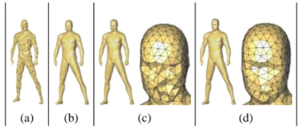
one by one in sequence, we cannot use the rebuilding scheme. We run it on a set of about13.000 points in a sphere (snodt) and on a surface mesh of a human body of about8.000 points (man). Figure 3 shows man at different iterations of the process. Close-ups on the head visually indicates that100 iterations are clearly not sufficient to get an high quality mesh (as confirmed by less visual quality measures).
(a) (b) (c) (d)
Figure 3: In (a) man initially; In (b), (c) and (d) man after 10, 100 and 1000 iterations respectively. (c) and (d), show close-ups on the head.
Experiments show a good convergence of the average tolerance of bi-cells to a reasonable value and of the aver-age tolerance of vertices to a smaller value, although these tolerances converge slower than in two dimensions.
For a random point distribution and random displace-ments of length δ, if displacedisplace-ments are small enough, and only around25% of the vertices have displacement above tolerance in two dimensions (55% in three dimensions), then T is competitive with rebuilding. In three dimensions, placement is twice slower and around nine time slower than rebuilding in two and three dimensions respectively. In extreme configurations, our algorithm outperforms re-building by a factor of17 (125 in three dimensions). How-ever those configurations are artificial and very unlikely to happen for real data sets.
The performance of T depends on the amount of dis-placements remaining inside the tolerance region. An idea of what this percentage represents in terms of distances can be shown within the context of random walk. When displacement magnitudes are around20% of avg(ǫ(V )) of the input set, T is still able to outperform rebuilding in both two and three dimensions. In three dimensions, if all dis-placements magnitudes are lower or equal to avg(ǫ(V )), T is more than three time faster than placement.
We now discuss the performance of the algorithms for Lloyd iterations, considering a thousand of iterations. We implemented in addition a small variation of the tolerance algorithm, suggested in Section 3, which consists of re-building for the first few iterations, and, swapping to T. We denote this algorithm by R+T.
In two dimensions, T and R+T outperform both rebuild-ing and placement. In three dimensions, they outperform placement in all configurations. This enhancement is rel-evant for applications requiring to move vertices one at a time and for dynamic triangulations, which cannot be achieved by rebuilding. However, to outperform rebuild-ing is harder in three dimensions, because the removal
op-eration is even slower and the number of bi-cells contain-ing a given point is five times larger than in two dimen-sions. In spite of that, T still outperforms rebuilding in synthetic and real data sets (snodt and man). T cannot perform with slloyd, as well as it does with the other in-puts, because of the slivers produced by running a pure Lloyd iteration (tolerances are sensitive to slivers). In both two and three dimensions, when we go further on the num-ber of iterations, T becomes faster. As shown in Figure 3, the number of iterations highly impacts the quality of the final result. This result enables a novel possibility: Going further on the number of iterations. More details on ex-perimental results are available in the full version of the paper [3].
5 Conclusion
This paper deals with the problem of updating Delaunay triangulations for moving points. We introduce the notion of the tolerance and safe region of a vertex in this context. We end up with an algorithm suitable when the magnitude of the displacement keeps decreasing while the tolerances keep increasing. Such configurations translate into conver-gent schemes, e.g. Lloyd’s iterations itself.
References
[1] Alliez P., Cohen-Steiner D., Yvinec M., and Desbrun M. Variational tetrahedral meshing. ACM Trans. on Graphics, 24:617–625, 2005. SIGGRAPH ’2005 Conf. Proc. [2] N. Amenta, M. Bern, and D. Eppstein. Optimal point
place-ment for mesh smoothing. In Proc. 8th ACM-SIAM Sym-pos. Disc. Algo., pages 528–537, January 1997.
[3] De Castro P. M. M. and Devillers O. Delaunay triangu-lations for moving points. Research report, INRIA, 2008, http://hal.inria.fr/inria-00344053/.
[4] Debard J. B., Balp R., and Chaine R. Dynamic Delau-nay Tetrahedralisation of a Deforming Surface. The Visual Computer, page 12 pp, Aug. 2007.
[5] Devillers O. Improved incremental randomized Delaunay triangulation. In Proc. 14th Annu. ACM Sympos. Comput. Geom., pages 106–115, 1998.
[6] Du Q., Faber V., and Gunzburger M.. Centroidal voronoi tessellations: Applications and algorithms. SIAM Rev., 41(4):637–676, 1999.
[7] Ostrovsky R., Rabani Y., Leonard J. Schulman, and Swamy C. The effectiveness of Lloyd-type methods for the k-means problem. In FOCS ’06: Proc. of the 47th Annu. IEEE Sympos. on Found. of Comp. Sci., pages 165–176, Washington, DC, USA, 2006. IEEE Computer Society. [8] D. Russel. Kinetic Data Structures in Practice. PhD thesis,
Stanford Univ., 2007.
[9] Tournois J., Alliez P., Wormser C., and Desbrun M. Quality isotropic tetrahedron meshing with optimal Delaunay trian-gulations, 2008.