HAL Id: halshs-00196485
https://halshs.archives-ouvertes.fr/halshs-00196485
Submitted on 12 Dec 2007HAL is a multi-disciplinary open access
archive for the deposit and dissemination of sci-entific research documents, whether they are pub-lished or not. The documents may come from teaching and research institutions in France or abroad, or from public or private research centers.
L’archive ouverte pluridisciplinaire HAL, est destinée au dépôt et à la diffusion de documents scientifiques de niveau recherche, publiés ou non, émanant des établissements d’enseignement et de recherche français ou étrangers, des laboratoires publics ou privés.
velocity of money
Olivier Allain
To cite this version:
Olivier Allain. Monetary circulation, the paradox of profits, and the velocity of money. Third Interna-tional Biannual Conference on “Post-Keynesian Economic Policies”, CEMF, Université de Bourgogne, Dijon, 29 Nov.-1 Dec. 2007, Dec 2007, Dijon, France. �halshs-00196485�
and the velocity of money
Olivier ALLAIN
Université Paris Descartes et Centre d’Economie de la Sorbonne olivier.allain@univ-paris5.fr
Contribution to the International Conference “Principles of Post-Keynesian Economic Policies”, CEMF, Université de Bourgogne, Dijon, France, November 30 - December 1, 2007
Abstract. Recent papers have reconsidered the paradox of profits, that is the difficulty to explain how monetary profits can be generated when firms borrow only the wage bill to finance their production. In this article, we use a stock-flow consistent approach give a solution to this paradox assuming that, when firms sell goods at prices which exceed their unit costs, the realised monetary profits are not used to pay back banks. These profits then remain in the circuit, allowing additional transactions. In a sense, profits result from their own expenditure. According to this interpretation, the velocity of money is higher than one because some monetary units are used in several transactions of goods.
Key words: paradox of profits, circulation, endogenous money, velocity of money, stock-flow consistent approach
The question of the realisation of monetary profits is regularly addressed in the
theoretical debates which rest on the endogenous money hypothesis.2 According to this
hypothesis, a distinction may be made between initial and final finance (Graziani, 1987). The former rests on Keynes’s finance motive, that is the money creation which starts the production process by financing production costs. The latter concerns the financing of investment expenditures.
In this framework, the ‘paradox of profits’ may be posed in the following terms: “if in an economic system (closed to external exchange) the only money existing is what the banks create in financing production, the amount of money that firms may hope to recover by selling their products is at the most equal to the amount by which they have been financed by banks. Therefore, once the principal has been repaid to banks, the possibility that firms as a whole can realise their profits in money terms or can pay interest owed to banks in money terms is ruled out” (Zazzaro, 2003, p. 233).
1 We would like to thank Nicolas Canry, Claude Gnos, Marc Lavoie, Louis-Philippe Rochon and
Franck Van de Velde for their helpful comments and suggestions. Of course, all remaining errors are ours.
2 See the recent contributions by Renaud (2000), Nell (2002), Gnos (2003), Seccarecia (2003),
Several solutions to the paradox of profits have been proposed in the literature.3 According to Nell (2002, p. 520), “it is necessary to show how the system can work without reliance on outside assistance”. We therefore do not retain the solutions which rest on the inclusion of an external sector (the government or the rest of the world) nor those which
assume the existence of several overlapping circuits.4
Some other solutions relate on the assumption that money creation covers both the wage bill and the investment expenditure (Seccarecia, 2003; Parguez, 2004; Rochon, 2005). Besides solving the paradox of profits, the advantages of this solution would be twofold. Firstly, it ensures that investment is autonomous and does not depend on saving behaviour such as hoarding. Secondly, as pointed by Seccarecia (2003), this solution appears to be realistic according to the fact that investment is actually financed by bank credit more than by selling equities to households.
Let us note that, in this solution, initial financing of investment is double: money is created to pay wages in the capital goods sector; and money is created to allow firms to buy capital goods. Yet, according to Nell (2002), this solution is expensive for firms which must pay interests to banks. Moreover, assuming no saving on wages, money creation equals the
nominal income of the economy.5 In other words, the ‘velocity of money’6 is equal to one:
every monetary unit is used in only one transaction of goods before it is destroyed. Indeed, firms’ receipts are immediately and entirely used to pay back the initial loans.
As a result of these remarks, the aim of this article is to present an alternative solution which is consistent with the assumption that initial finance is restricted to the wage bill. This solution requires showing how some monetary units are used in several transactions of goods: because firms sell their output at prices which exceed unit costs, they can pay back production costs to banks while profits remain in the circuit where they are used in other transactions. Then, velocity of money is higher than unity and monetary profits are positive. Eventually, profits result from their own expenditure.
Of course this conclusion is not really original. It appears in Leonard (1987) and in Renaud (2000), but their arguments are not entirely satisfying because the authors do not attach enough importance to the velocity of money. On the contrary, this issue plays a central role in Nell (2002, 2004). Moreover, Nell takes a very restrictive hypothesis, assuming that advances cover only the wage bill of the capital goods sector. He proposes an extensive proof, but he adopts two assumptions that we do not retain: consumption goods are produced in the previous period, and there is a ‘machine tools’ sector which makes its own capital goods. Finally, our interpretation is very close to the one that is sketched by Gnos and Schmitt (1990) and Gnos (2003). Our main contribution lies in the attempt to give a formal proof. According to our above argument, we will assume a succession of transactions ‘rounds’ in the same period and we will track monetary as well as real flows throughout the period. To do this, we use the stock-flow consistent accounting proposed by Godley (1996, 1999), Lavoie (2004),
3 See Rochon (2005) for a survey.
4 In the latter case, the system provides always enough money to realise monetary profits. A variant
is proposed by Messori and Zazzaro (2005) who explain that, in a growing economy, firms are not at the same stage of their life cycle: those which go bankrupt do not pay back the banks; start-ups need large loans and do not make profits. Therefore money remains available that enables other firms to realise profits.
5 Indeed, ΔM=W+I=C+I. A problem arises when there is saving on wages because ΔM=W+I>
C+I, that is money creation is greater than the nominal income.
6 Following Nell (1990), velocity of money “is measured by the ratio of money income and the
stock of money [which corresponds to] the number of times the stock of money turned over in the course of the transactions making up the period’s income” (p. 37).
and Godley and Lavoie (2007). This method guarantees that every monetary flow comes from somewhere and goes somewhere, so that there is no ‘black hole’ in the accounts. It thus makes it possible to check that any expenditure rests on prior detention of money.
We will see that our argument may be consistent with the observation that final financing of investment rests on bank credit. Moreover, a velocity of money higher than unity improves the realism of the argument.
The first section is devoted to methodological remarks. We then address the paradox of profits before solving it in the third section. We explore some variations in the fourth section. The last section presents our conclusions.
1. Methodological remarks
We adopt a very simple economic model with only three agents: households allocate their income between consumption and saving; firms produce consumption and capital goods, distribute all their profits (if any), and finance their investment expenditures by issuing equities to capture households’ saving; banks play a passive role by creating the money required by firms to pre-finance production. The amount of pre-financing corresponds exactly to the wage bill. Moreover, we assume that there is interest neither on loans nor on deposit. Note that most of these hypotheses will be relaxed in the fourth section.
This article does not focus on production nor investment decisions. On these issues, we adopt the Keynes’s principle of effective demand and we assume that investment is exogenous. Moreover, we use Keynes’s distinction between short and long-term expectations. Accordingly, short-term expectations “[are] concerned with the price which a manufacturer can expect to get for his ‘finished’ products at the time when he commits himself to starting the process which will produce it” (Keynes, 1936, p. 46). However, for sake of clarity, we most of the time suppose that the short-term expectations are fulfilled.
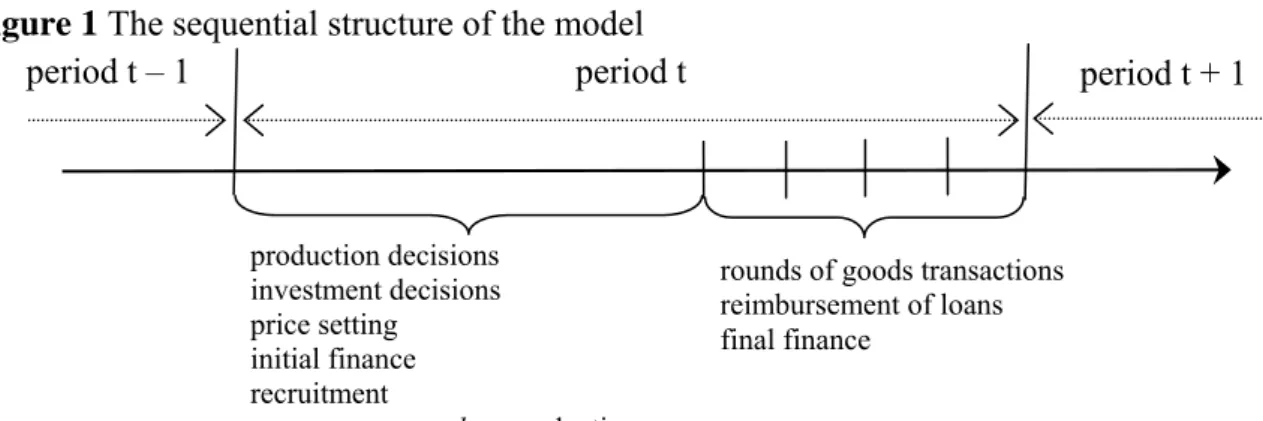
Figure 1 The sequential structure of the model
period t – 1 period t production decisions investment decisions price setting initial finance recruitment then production
rounds of goods transactions reimbursement of loans final finance
period t + 1
In this framework, our aim is to understand how, over a given period, a quantity of money initially equal to the wage bill will make all the transactions possible and ensure the realisation of profits before being destroyed when the loans are paid back. To answer this question, we adopt a sequential approach in which each period is divided into two sub-periods (cf. Figure 1). In the first sub-period, firms set the level of production, hire workers, and produce goods. They also plan their investment expenditure. At the end of this sub-period, the produced goods have to be kept as inventories while waiting to be sold. The second sub-period is devoted to the sale of goods, the financing of investment and the paying back of initial loans. This second sub-period is itself divided in several rounds, which makes it possible to precisely follow monetary flows and to make sure that each agent’s expenditure rests on an effective detention of money. At the end of each round, firms use all or part of
their receipts to pay the banks back. Rounds follow one another until inventories and/or bank deposits are exhausted.
Note that the analysis could be carried out by distinguishing the sector of consumption goods and that of capital goods (Nell, 2002, 2004). But this is not necessary. However, it is crucial to assume that firms cannot accumulate the capital goods they have produced themselves (other than as inventories). If so, investment would be the counterpart of profits in kind. Yet, to be sure to exhibit monetary profits, investment must be the counterpart of a transaction.
2. The paradox of profits
In this section, we use Godley and Lavoie’s stock-flow consistent accounting to expose the paradox of profits in its simplest version.
At the beginning of the first sub-period, entrepreneurs anticipate the demand of goods (Q) and set up employment level (N). The monetary wage (w) being given, the wage bill is W =wN. Firms borrow this amount to banks (∆L0) and pay workers who deposit their wages on a
bank account (∆M0). Workers produce goods which are kept as inventories (IN0) before being
sold.7 As underlined by Godley (1996), inventories must be assessed at their production costs
to preserve accounting identities. We thus have:
∆L0 = ∆M0 = IN0 = W (1)
These flows are recorded in Table 1. According to Godley and Lavoie, variables with a sign plus represent a source of funds whereas variables with a negative sign represent the use of funds; every line and column must sum to zero to guarantee that each funds has a source
and a destination.8
Table 1
Transactions matrix: end of the first sub-period
Households Firms Banks
Current Capital Capital ∑
Consumption (C0) 0 Investment (I0) 0 Inventories (IN0) + W – W 0 Wages (W) + W – W 0 Profits (Π0) 0 ∆ in loans (∆L0) + W – W 0 ∆ in money (∆M0) – W + W 0
Issue of equities (∆E0) 0
∑ 0 0 0 0 0
During the first round of the second sub-period, households spend the fraction c of their
deposits to buy consumption goods (C1 =cW). The remainder is saved by buying equities.
This saving ensures the financing of part of the investment, that is I1 = ∆E1 = (1–c)W. As
previously underlined, investment must be the counterpart of a transaction, as is shown in the line ‘Investment’ in all the Tables below.
At the end of this round, all the wages go back to firms. The paradox of profits lies in the assumption that firms totally pay back their advances at this moment. The whole period
7 The flows ∆L, ∆M and IN are indexed to 0 because their amount will change during the second
sub-period. On the other hand, the flows Q, N and W are not indexed because they remain unchanged throughout the period.
ends because all the money is destroyed. Every monetary unit was used in only one transaction of goods before its destruction. The velocity of money (v) is thus equal to one.
At the end of the period, two situations may arise. In the first one, the stocks of inventories are exhausted (Table 2), which implies that goods were sold at their unit wage
cost (p=W/Q). So the monetary profits (Π) are nil.
Table 2
Transactions matrix:a end of the first round and of the period (situation 1)
Households Firms Banks
Current Capital Capital ∑
Consumption (C) – cW + cW 0 Investment (I) + (1–c)W – (1–c)W 0 Inventories (IN) 0 Wages (W) + W – W 0 Profits (Π) 0 ∆ in loans (∆L) 0 ∆ in money (∆M) 0
Issue of equities (∆E) – (1–c)W + (1–c)W 0
∑ 0 0 0 0 0
a Note that a transactions matrix is not limited to the flows of a given round, but it takes into account all the net flows since the beginning of the period. That explains why wages, which are paid during the first sub-period, continue to appear in each Table in the article.
The second situation is more complex because it rests on the hypothesis that each good
was sold at a price which exceeds its production cost, that is:9
(
)
Q W
p= 1+θ (2)
This hypothesis affects the model in the following way (cf. Table 3): during the first
round, as previously, total expenditure equals the wage bill (that is C1 +I1 =W). This
expenditure corresponds to the receipts pQ1, where Q1 represents the volume of goods drawn
from inventories. Replacing p, C1 and I1 leads to:
π θ = − + = ⇔ + = 1 1 1 1 1 1 1 Q Q I C pQ (3)
where π =θ
(
1+θ)
. Since Q1 Q is lower than unity, inventories are not exhausted. Inother words, an amount of wages equals to
(
1−π)
W was sufficient to obtain pQ1. Thesereceipts thus generate some monetary profits:
(
)
W WpQ − −π =π =
Π1 1 1 (4)
Moreover, the value of the remaining inventories (measured at production costs) amounts to: W W Q Q IN ⎟⎟ =π ⎠ ⎞ ⎜⎜ ⎝ ⎛ − = 1 1 1 (5)
Consequently, the monetary profits realised with the sale of Q1 is exactly balanced by
the production costs of the remaining inventories. Resulting monetary profits are nil again,
9 It is not necessary to give a functional form for the production function. In the case of factor
substitution, the term (1+θ) is equal to the ratio between marginal and unit costs; it may be regarded as given since it results from decisions taken by entrepreneurs at the beginning of the period. In the case of a fixed coefficient production function, θ simply represents the mark-up rate.
although the value of income reaches (1+π)W and exceeds the wage bill. Stocks of
inventories then correspond to a profit in kind.
Table 3
Transactions matrix: end of the first round and of the period (situation 2)
Households Firms Banks
Current Capital Capital ∑
Consumption (C1) – cW + cW 0 Investment (I1) + (1–c)W – (1–c)W 0 Inventories (IN1) + πW – πW 0 Wages (W) + W – W 0 Profits (Π1) – πW + πW 0 ∆ in loans (∆L1) 0 ∆ in money (∆M1) 0
Issue of equities (∆E1) – (1–c)W + (1–c)W 0
∑ 0 0 0 0 0
3. A solution of the paradox
The central hypothesis to solve the paradox is to assume that firms do not use their
monetary profits (πW) to pay their debt back. The remaining amount (that is
(
1−π)
W) maybe used to begin to pay back the banks as well as it may be deposit on an account while waiting to recover the whole advances. Whatever the choice, it does not affect the results of the analysis. We adopt the second one for sake of simplicity.
Another assumption may be added, although it is not fundamental and will be relaxed later: we suppose that profits are distributed to households which deposit them at the bank.
Eventually, one may check that deposits and loans remain equal (ΔM1 ≡ΔL1). The situation
at the end of the first round is displayed in Table 4.
Table 4
Transactions matrix: end of the first round
Households Firms Banks
Current Capital Capital ∑
Consumption (C1) – cW + cW 0 Investment (I1) + (1–c)W – (1–c)W 0 Inventories (IN1) + πW – πW 0 Wages (W) + W – W 0 Profits (Π1) + πW – πW 0 ∆ in loans (∆L1) + W – W 0 ∆ in money (∆M1) – πW – (1–π)W + W 0
Issue of equities (∆E1) – (1–c)W + (1–c)W 0
∑ 0 0 0 0 0
The same process applies to the second round (cf. Table 5): households consume part of the profits they have just received, while firms issue equities to collect new saving and carry on with their investments. By adding these expenditures to those of the first round
(C2 =C1 +cΠ1 et I2 =I1 +(1–c)Π1), it results that C2 +I2 =(1+π)W. One can calculate Q2 Q
the proportion of the total volume of goods drawn from inventories, that is:
(
π θ + + = ⇔ + = 1 1 1 2 2 2 2 Q Q I C pQ) (6)
As previously underlined, this fraction corresponds to the fraction of the wage bill
which was necessary to produce Q2 and to generate the receipts pQ2. Since the beginning of
the period, cumulated profits have thus reached:
(
)
W W pQ 2 2 2 1 1 π π θ π = + + + − = Π (7)Moreover, the value of the remaining inventories amounts to:
W W Q Q IN 2 2 2 1 ⎟⎟ =π ⎠ ⎞ ⎜⎜ ⎝ ⎛ − = (8) Table 5
Transactions matrix: end of the second round
Households Firms Banks
Current Capital Capital ∑
Consumption (C2) – c(1+π)W + c(1+π)W 0 Investment (I2) + (1–c)(1+π)W – (1–c)(1+π)W 0 Inventories (IN2) + π2 W – π2 W 0 Wages (W) + W – W 0 Profits (Π2) + (π+π2)W – (π+π2)W 0 ∆ in loans (∆L2) + W – W 0 ∆ in money (∆M2) – π2 W – (1–π2)W + W 0
Issue of equities (∆E2) – (1–c)(1+π)W + (1–c)(1+π)W 0
∑ 0 0 0 0 0
The new profits (Π2 –Π1 =π2W) are distributed to households who deposit them on their
accounts. At the same time, firms put the residual part of receipts on their account. It results
that ΔM2 ≡ΔL2.
The next rounds progress in the same way: households consume and save the profits of the previous round; firms issue equities to capture the new saving and to pursue their
investments. However, after n rounds, IN L nW gradually vanishes:
n n =Δ =π
10 the period
ends when inventories are exhausted. At this stage, all the money returned back to firms which can pay back their whole advances (cf. Table 6). We thus have:
∑
=−
= ni i
n cW
C 1π 1 which converges towards C c
(
)
Wn = 1+θ , (9)
(
−)
∑
= − = n i i n cW I 1 11 π which converges towards In =
(
1−c)(
1+θ)
W , and (10)∑
==
Π n
i i
n W 1π which converges towards Πn =θW .
11 (11)
The paradox of profits is solved. The amount W of money creation leads to an amount
of transactions which reaches (1+θ)W. The velocity of money is thus v=1+θ. As underlined
by Nell (1990), “‘velocity’ turns out to be a reflection of the markup” (p. 33). Of course, the neoclassical interpretation of the quantity theory does not apply: in our argument, money creation is endogenous (depending on real output) and does not affect prices.
10 Note that the series quickly converge: when π is worth 0.4, inventories go down to 1% from their
initial amount in only five rounds.
11 Because profits are distributed and the propensity to save wages is positive, profits are higher
Table 6
Transactions matrix: end of the period
Households Firms Banks
Current Capital Capital ∑
Consumption (C) –c(1+θ)W +c(1+θ)W 0 Investment (I) +(1–c)(1+θ)W –(1–c)(1+θ)W 0 Inventories (IN) 0 Wages (W) + W – W 0 Profits (Π) + θW – θW 0 ∆ in loans (∆L) 0 ∆ in money (∆M) 0
Issue of equities (∆E) –(1–c)(1+θ)W +(1–c)(1+θ)W 0
∑ 0 0 0 0 0
At this stage, it is important to remind that our article does not focus on agents decisions. Firms are thus assumed to plan their investment as well as their production at the beginning of the period. Investment is assumed to be exogenous, depending on firms’ long-term expectations. On the other hand, production depends on firms’ expectations about the demand that they will have to face at the end of the period. In this section, we assumed that these short-term expectations were fulfilled. It implies that the final amounts of production
(pQ=(1+θ)W) and investment (I=(1–c)(1+θ)W) correspond to firms’ plans. Consequently,
production depends on the usual multiplier:
c I pQ − = 1 (12)
Moreover, although the amount of investment seems to depend on that of saving, the former is autonomous whereas the latter is endogenous. In other words, It implies that, whatever the amount of investment expenditure, it faces the corresponding amount of saving,
irrespective of the difficulty for firms to collect this saving.12
Of course, some problems may arise as soon as the prior hypotheses are relaxed: what happens if profits are not distributed, if firms have to pay dividends or interests, or if households prefer liquidity rather than equities? Also, what happens if entrepreneurs’ short-term expectations are not fulfilled? We will see in the next section that our solution remains available when we answer to these questions.
4. Variations
Errors in short-term expectations
Until then, entrepreneurs were supposed to fulfil their short-term expectations about their sales at the end of the period. Of course, expectations may be erroneous, and this in
several ways.13 Assume for instance that capital goods entrepreneurs underestimate their
sales: they could sell more than I=(1–c)(1+θ)W. However, they hire and produce
accordingly to their expectations, and the situation at the end of the period is the same as in Table 6. The only difference is that some planned investments are not carried out. The story is almost the same if consumption goods entrepreneurs underestimate their sales: they produce
as if the propensity to consume was c whereas it is c’ with c’>c. At the end of the period,
households cannot consume as much as they would like. They are forced to save so that their
12 For instance, a higher c does not result in a weaker saving but in a higher income.
13 We suppose here that prices are set by firms at the beginning of the period. The closure of the
model differs if prices are assumed to be set by the market at the end of the period (Allain, 2008), but this does not fundamentally affect the question of profits realisation.
propensity to consume decreases from c’ to c. The final situation is again displayed in Table 6.
Alternately, entrepreneurs may overestimate their sales. Assume that capital goods
entrepreneurs overestimate the demand they will have to face:14 for instance, they expected
I=(1–c)(1+θ)W while planned investment is limited to (1–c)(1+π)W. Then transactions
stops at the end of the second round (see Table 5). The only difference is that firms may issue
equities to capture households’ deposits (ΔM2 = π2W in Table 5) to pay back their advances
(Table 7). Eventually, capital goods firms have to keep some output as inventories and their profits are lower than expected.
Table 7
Transactions matrix: end of the period (overestimation of capital goods demand)
Households Firms Banks
Current Capital Capital ∑
Consumption (C) – c(1+π)W + c(1+π)W 0 Investment (I) + (1–c)(1+π)W – (1–c)(1+π)W 0 Inventories (IN) + π2 W – π2 W 0 Wages (W) + W – W 0 Profits (Π) + (π+π2)W – (π+π2)W 0 ∆ in loans (∆L) 0 ∆ in money (∆M) 0
Issue of equities (∆E) – [π2 +(1–c)(1+π)]W – [π2 +(1–c)(1+π)]W 0
∑ 0 0 0 0 0
Whatever the error in short-term expectations, two results must be underlined. On the one hand, the accounting identity between investment and saving remains fulfilled (provided that investment includes involuntary stocks of unsold goods if any). On the other hand, the outcome of the period must lead entrepreneurs to modify their expectations and behaviours at the beginning of the following period.
Undistributed profits
In the previous section, profits were assumed to be totally distributed to households. But profits can also be retained by firms. In this case, in order to follow every monetary flow, we assume that firms put the profits on their deposits at the end of each round (cf. Table 8).
Table 8
Transactions matrix: end of the first round (undistributed profits)
Households Firms Banks
Current Capital Capital ∑
Consumption (C1) – cW + cW 0 Investment (I1) + (1–c)W – (1–c)W 0 Inventories (IN1) + πW – πW 0 Wages (W) + W – W 0 Profits (Π1) – πW + πW 0 ∆ in loans (∆L1) + πW – πW 0 ∆ in money (∆M1) – πW + πW 0
Issue of equities (∆E1) – (1–c)W + (1–c)W 0
∑ 0 0 0 0 0
From the second round onward, firms finance their investments by using their deposits. Besides, there is no additional consumption because households do not receive any additional income. However, the sale of capital goods makes it possible to realise new profits which are
used in the following periods to pursue investment expenditures. The final transactions matrix is given in Table 9.
Table 9
Transactions matrix: end of the period (undistributed profits)
Households Firms Banks
Current Capital Capital ∑
Consumption (C) – cW + cW 0 Investment (I) + (1–c+θ)W – (1–c+θ)W 0 Inventories (IN) 0 Wages (W) + W – W 0 Profits (Π) – θW + θW 0 ∆ in loans (∆L) 0 ∆ in money (∆M) 0
Issue of equities (∆E) – (1–c)W + (1–c)W 0
∑ 0 0 0 0 0
The total income, as well as its distribution between wages and profits, is identical to that of the previous section. But, the part of output devoted to investment is higher. This results from a weaker propensity to consume the income because all the profits are saved. Indeed, the multiplier becomes:
θ + − = 1 1 c I pQ (13)
The multiplier is therefore lower as previously. It means that the level of investment must be higher to reach the same levels of output and employment. Moreover, note that investment is not solely financed by profits. It would only be the case if households totally
consume their wages (that is, if c=1). Of course, some firms may invest less than their whole
profits. Then they distribute the remaining part of their profits. Table 9 must be mixed with Table 6 to display this case.
Dividends, interests, and bank behaviour
We indirectly dealt with the question of dividends by supposing that profits were entirely distributed to households. The question of interests is trickier, especially since some authors (Leonard, 1987; Zezza, 2004) gave it a central place in the paradox of profits. Let us solve this question by assuming that banks do not pay any interest on deposits, but that they withdraw interests (at the rate r) on current loans. Under those hypotheses, the amount of interests is rW. Moreover, a new line and a new column must be added to the transactions matrix (cf. Table 10). The new column corresponds to the current account of banks. The stock-flow consistent approach makes it possible to make sure that every flow of interests collected by the banks will have a counterpart: as pointed out by Zezza (2004, p. 3), the uses may be the payment of wages, the payment of interests on deposits, or the realisation of banking profits which may either be distributed to households or used to buy equities or capital goods.
However, all these uses have the same property: the interests deduced from the receipts by firms come back to them as consumption expenditures (wages, interests on deposits, banking profits distributed to households), as investment expenditures (purchase of capital goods), or as saving which they capture by issuing equities. In Table 10, the interests on loans are supposed to generate banking profits which are entirely distributed to households.
Table 10
Transactions matrix: end of the period (interests on loans)
Households Firms Banks
Current Capital Current Capital ∑
Consumption (C) –c(1+θ)W +c(1+θ)W 0 Investment (I) +(1–c)(1+θ)W –(1–c)(1+θ)W 0 Inventories (IN) 0 Wages (W) + W – W 0 Profits (Π) + θW – (θ–r)W – rW 0 Interests on loans – rW +rW 0 ∆ in loans (∆L) 0 ∆ in money (∆M) 0
Issue of equities (∆E) –(1–c)(1+θ)W +(1–c)(1+θ)W 0
∑ 0 0 0 0 0 0
Interests are neutral in the sense that they do not constitute a leakage from the monetary
circuit.15 Nevertheless they affect the decisions of every entrepreneur who is not sure that the
interests he paid will come back to him in the form of expenditures: a rise of r may involve a fall of activity, regardless of its possible impact on the investment decisions.
In the same way, activity falls if banks do not satisfy all the demands of loans at the rate
r. This rationing reduces the ex ante financing of production at the beginning of the period
and not the ex post financing of investment (Lavoie, 2004).
Households’ liquidity preference
Let us here assume that households consume the part c of their income, keep the part λ
as deposits, and use the remaining part (1–c–λ≥0) to buy equities. Under those hypotheses,
the consumption after n rounds amounts to:
(
)
[
]
∑
= − − = in i n cW C 1 1 λ π 1This series converges towards:
(
)
W c Cn = 1+Ω where(
(
)
)
π λ π λ − − − = Ω 1 1 1The same calculations carried out on the other variables lead to the situation described in Table 11.
Table 11
Transactions matrix: after n rounds (households’ liquidity preference)
Households Firms Banks
Current Capital Capital ∑
Consumption (Cn) –c(1+ Ω)W +c(1+ Ω)W 0 Investment (In) + (1– c– λ)(1+ Ω)W – (1– c– λ)(1+ Ω)W 0 Inventories (INn) +λ(1+ Ω)W –λ(1+ Ω)W 0 Wages (W) + W – W 0 Profits (Πn) +ΩW –ΩW 0 ∆ in loans (∆Ln) +W –W 0 ∆ in money (∆Mn) –λ(1+ Ω)W –[1– λ(1+ Ω)]W +W 0
Issue of equities (∆En) – (1– c– λ)(1+ Ω)W + (1– c– λ)(1+ Ω)W 0
∑ 0 0 0 0 0
Firms do not collect enough saving to entirely finance their investment expenditures. Nevertheless, creating additional money is not necessary since banks can play their role of
15 This explains why Tables 6 and 10 differ only by the distribution of profits between firms and
financial intermediation by transforming households’ deposits into loans. These new loans start the monetary circuit again: the investment expenditures of some firms make it possible for others to continue to pay back the banks and make profits; these profits are distributed to households who use them to consume and to save (in the form of money and equities), etc. The process goes on until inventories are exhausted. The final situation is given in Table 12. Because of hoarding, firms cannot totally repay the banks. Thus production must partly be
financed by long-term loans.16
If we correctly understand Rochon’s (2005) argument, this result contributes to assume that advances cover both wages and investment. Of course, firms must be sure that banks will extend some loans over several periods. However, no additional money has to be created at the beginning of the period to close the circuit. Under a perfect short-term expectations hypothesis, as loans are expensive (Nell, 2002, 2004), it would be sufficient to borrow W and to make a distinction between short and long-term loans. In an uncertain world, firms may be tempted to borrow more than W. Nevertheless, Keynes (1936, ch.5) himself appears confident with regard to the existence of a trial and error procedure that brings entrepreneurs to optimal short-term decisions. Although planned investment has to be secured at the beginning of the
period, this does not imply that money creation cover both wages and investment.17
Table 12
Transactions matrix: end of the period (households’ liquidity preference)
Households Firms Banks
Current Capital Capital ∑
Consumption (C) –c(1+θ)W +c(1+θ)W 0 Investment (I) +(1–c)(1+θ)W –(1–c)(1+θ)W 0 Inventories (IN) 0 Wages (W) + W – W 0 Profits (Π) + θW – θW 0 ∆ in loans (∆L) + λ(1+θ)W – λ(1+θ)W 0 ∆ in money (∆M) – λ(1+θ)W + λ(1+θ)W 0
Issue of equities (∆E) – (1– c– λ)(1+θ)W + (1– c– λ)(1+θ)W 0
∑ 0 0 0 0 0
Amount of initial finance and velocity of money
In the monetary circuit approaches, it is generally admitted that the amount of initial finance must cover the wage bill. It is easy to show that this is not necessary. Let us assume
that firms borrow a fraction α (α<1) of the wage bill either because they only pay part of the
wages to each worker at the beginning of the period or because they only hire part of the
workers.18 Under these hypotheses, the previous results hold, provided that firms use their
receipts (net of profits) to pay the remaining wages (or to complete the recruitment) before they begin to pay back the banks.
16 See Van de Velde (2005) on this point.
17 Rochon’s (2005) argument partly rests on Keynes’s quotations according to which “planned
investment (…) may have to secure its ‘financial provision’ before (…) the corresponding saving has taken place” (Keynes, 1937, p. 246). It is not sure that this quotation helps Rochon’s aim because Keynes (1937, pp. 245-46) explains that the financial provision (which can take the form of a revolving fund) does not necessarily imply a money creation. Moreover, this financial provision has to solve a problem in the short-term, not in the long-term.
18 With this hypothesis, our argument is very similar to Nell’s (2002, 2004) who assumes that
The firms’ deposits at the end of the first round (cf. the cell in Table 13) represent the part of the receipts which could be used to pay back the loans but which are used to raise the wage bill.
f
M1
Δ
Table 13
Transactions matrix: end of the first round (partial initial financing of the wage bill)
Households Firms Banks
Current Capital Capital ∑
Consumption (C1) – cαW + cαW 0 Investment (I1) + (1–c)αW – (1–c)αW 0 Inventories (IN1) + παW – παW 0 Wages (W) + αW – αW 0 Profits (Π1) + παW – παW 0 ∆ in loans (∆L1) + αW – αW 0 ∆ in money (∆M1) – παW – (1–π)αW + αW 0 Issue of equities (∆E1) – (1–c)αW + (1–c)αW 0
∑ 0 0 0 0 0
The same process applies during the next rounds until the total wage bill W is reached. Then the previous analysis applies again. At the end of the period, firms can pay back their initial loans (αW). The final matrix corresponds to Table 6. The main difference lies in a greater number of rounds. The monetary units thus circulate more quickly which means that
the velocity of money is v= 1
(
+θ)
α.5. Conclusion
In this article, we show that the paradox of profits may be solved even if advances are limited to wages. The main hypothesis then is to assume that, when a firm sells a good, the ‘markup’ is not used to pay back banks. Therefore, profits remain in the circuit and generate new transactions. The money is thus reinjected several times in the circuit before being destroyed. Two core conclusions must be underlined: firstly, profits are generated by their own expenditures; secondly, the velocity of money is higher than unity.
Moreover, the argument is consistent with Seccarecia’s (2003) concerns about the realism of final financing of investment: it may be provided by an issue of equities as well as by undistributed profits; also, it has to be financed by banks in the case of hoarding. However, in the latter case, bank credit may take the form of financial intermediation rather than of money creation.
Of course, the present solution does not prevent some other solutions of the paradox of profits.
Bibliography
Allain O. (2008) “Effective Demand and Short-term Adjustments in the General Theory”,
Review of Political Economy, forthcoming.
Gnos C. (2003) “Circuit Theory as an Explanation of the Complex real World”, in L.P. Rochon and S. Rossi (eds) Modern Theories of Money: the nature and the Role of money
in Capitalist Economy, Cheltenham, Edward Elgar, pp. 322-38.
Gnos C., Schmitt B. (1990) “Le circuit, réalité exhaustive”, Economies et Sociétés (Série
Godley W. (1996) Money, Finance and National Income Determination: An Integrated
Approach, Annandale-on-Hudson (USA), The Levy Economics Institute, Working Paper
n° 167.
Godley W. (1999) “Money and Credit in a Keynesian Model of Income Determination”,
Cambridge Journal of Economics, 23, pp. 393-411.
Godley W., Lavoie M. (2007) Monetary Economics: An Integrated Approach to Credit,
Money, Income, Production and Wealth, Palgrave MacMillan.
Graziani A. (1987) “Keynes’ Finance Motive”, Economies et Sociétés (Série Monnaie et
Production), 9, pp. 23-42.
Keynes J. M. (1936) The General Theory of Employment, Interest and Money, London, Macmillan.
Keynes J.M. (1937) “Alternative theories of the rate of interest”, The Economic Journal, 47(186), pp. 241-52.
Lavoie M. (2004) “Circuit and Coherent Stock-Flow Accounting”, in R. Arena and N. Salvadori (eds) Money, Credit and the Role of the State, Aldershot, Ashgate, pp. 136-51. Leonard J. (1987) “Le paradoxe de l’intérêt et la crise de l’économie monétaire de
production”, Economies et Sociétés (Série Monnaie et Production), 4, pp. 149-68.
Messori M., Zazzaro A. (2005) “Single Period Analysis: Financial Markets, Firms’ Failures and the Closure of the Monetary Circuit”, in G. Fontana and R. Bellofiore (eds) The
Monetary Theory of Production: Tradition and Perspectives, London, Macmillan.
Nell E.J. (1990) “The quantity theory and the mark-up equation”, Economie Appliquée, XLIII(2), pp. 33-42.
Nell E.J. (2002) “On Realizing Profits in Money”, Review of Political Economy, 14(6), pp. 519-30.
Nell E.J. (2004) “Monetising the Classical Equations: a theory of circulation”, Cambridge
Journal of Economics, 28, pp. 173-203.
Parguez A. (2004) “The Solution of the Paradox of Profits”, in R. Arena and N. Salvadori (eds) Money, Credit and the Role of the State, Aldershot, Ashgate, pp. 257-70.
Renaud J.-F. (2000) “The Problem of the Monetary Realization of Profits in a Post Keynesian Sequential Financing Model: two solutions of the Kaleckian option”, Review of Political
Economy, 12(3), pp. 285-303.
Rochon L.-P. “The Existence of Monetary Profits within the Monetary Circuit: An Essay in Honour of Augusto Graziani”, in G. Fontana and R. Bellofiore (eds) The Monetary
Theory of Production: Tradition and Perspectives, London, Macmillan.
Seccarecia M. (2003) “Pricing, Investment and the Financing of Production within the framework of the Monetary Circuit: Some Preliminary Evidence”, in L.P. Rochon and S. Rossi (eds) Modern Theories of Money: the nature and the Role of money in Capitalist
Economy, Cheltenham, Edward Elgar, pp. 173-97.
Van de Velde F. (2005) Monnaie, chômage et capitalisme, Villeneuve d’Ascq, Presses Universitaires du Septentrion.
Zazzaro A. (2003) “How Heterodox is the Heterodoxy of Monetary Circuit Theory? The Nature of Money and the Microeconomics of the Circuit”, in L.P. Rochon and S. Rossi
(eds) Modern Theories of Money: the nature and the Role of money in Capitalist
Economy, Cheltenham, Edward Elgar, pp. 219-45.
Zezza G. (2004) Some Simple, Consistent Models of the Monetary Circuit, Annandale-on-Hudson (USA), The Levy Economics Institute, Working Paper n° 405.