HAL Id: hal-00487520
https://hal.archives-ouvertes.fr/hal-00487520
Submitted on 29 May 2010
HAL is a multi-disciplinary open access
archive for the deposit and dissemination of
sci-entific research documents, whether they are
pub-lished or not. The documents may come from
teaching and research institutions in France or
abroad, or from public or private research centers.
L’archive ouverte pluridisciplinaire HAL, est
destinée au dépôt et à la diffusion de documents
scientifiques de niveau recherche, publiés ou non,
émanant des établissements d’enseignement et de
recherche français ou étrangers, des laboratoires
publics ou privés.
Optimized Schwarz Methods for Maxwell’s Equations
with Non-Zero Electric Conductivity
Victorita Dolean, Mohamed El Bouajaji, Martin Gander, Stephane Lanteri
To cite this version:
Victorita Dolean, Mohamed El Bouajaji, Martin Gander, Stephane Lanteri. Optimized Schwarz
Meth-ods for Maxwell’s Equations with Non-Zero Electric Conductivity. 2010. �hal-00487520�
Equations with Non-Zero Electric Conductivity
Victorita Dolean1, Mohamed El Bouajaji2, Martin J. Gander3 and St´ephane
Lanteri2
1 Laboratoire J.A. Dieudonn´e, CNRS UMR 6621, F-06108 Nice Cedex, France
2 Nachos project-team, INRIA Sophia Antipolis - M´editerran´ee research center,
F-06902 Sophia Antipolis Cedex, France
3 Mathematics Section, University of Geneva, CH-1211, Geneva, Switzerland
1 Introduction
The study of optimized Schwarz methods for Maxwell’s equations started with the Helmholtz equation, see [3, 4, 2, 11]. For the rot-rot formulation of Maxwell’s equations, optimized Schwarz methods were developed in [1], and for the more general form in [9, 10]. An entire hierarchy of families of optimized Schwarz methods was analyzed in [8], see also [5] for discontinuous Galerkin discretizations and large scale experiments. We present in this paper a first analysis of optimized Schwarz methods for Maxwell’s equations with non-zero electric conductivity. This is an important case for real applications, and requires a new, and fundamentally different optimization of the transmission conditions. We illustrate our analysis with numerical experiments.
2 Schwarz Methods for Maxwell’s Equations
The time dependent Maxwell equations are −ε∂E∂t + curl H − σE = J, µ∂H
∂t + curl E = 0, (1) where E = (E1,E2,E3)T and H = (H1,H2,H3)T denote the electric and
mag-netic fields, respectively, ε is the electric permittivity, µ is the magmag-netic per-meability, σ is the electric conductivity and J is the applied current density. We assume the applied current density to be divergence free, divJ = 0.
One can show, see for example [8] for the context of domain decomposition methods, that the time dependent Maxwell equations (1) are a system of hyperbolic partial differential equations. This hyperbolic system has for any interface two incoming and two outgoing characteristics. Imposing incoming characteristics is equivalent to imposing the impedance condition
2 V. Dolean et al.
Bn(E, H) := n ×ZE + n × (H × n) = s. (2) We consider in this paper the time-harmonic Maxwell equations,
−iωεE + curl H − σE = J, iωµH + curl E = 0. (3) A family of Schwarz methods for (3) with a possibly non-overlapping decom-position of the domain Ω into Ω1 and Ω2, with interfaces Γ12 := ∂Ω1∩ Ω2
and Γ21:= ∂Ω2∩ Ω1, is given by −iωεE1,n+curl H1,n −σE1,n= J in Ω 1, iωµH1,n+ curl E1,n= 0 in Ω1, (Bn1+S1Bn2)(E 1,n, H1,n) = (Bn 1+S1Bn2)(E 2,n−1, H2,n−1) on Γ 12, −iωεE2,n+curl H2,n −σE2,n= J in Ω 2, iωµH2,n+ curl E2,n= 0 in Ω2, (Bn2+S2Bn1)(E 2,n, H2,n) = (Bn 2+S2Bn1)(E 1,n−1, H1,n−1) on Γ 21, (4)
where Sj, j = 1, 2 are tangential, possibly pseudo-differential operators.
Dif-ferent choices of Sj, j = 1, 2 lead to different parallel solvers for Maxwell’s
equations, see [8]. The classical Schwarz method is exchanging characteris-tic information at the interfaces between subdomains, which means Sj = 0,
j = 1, 2. For the case of constant coefficients and the domain Ω =R3, with
the Silver-M¨uller radiation condition lim
r→∞r (H× n − E) = 0, (5)
and the two subdomains
Ω1= (0, ∞) × R2, Ω2= (−∞, L) × R2, L≥ 0, (6)
the following convergence result was obtained in [8] using Fourier analysis: Theorem 1. For any (E1,0; H1,0) ∈ (L2(Ω
1))6, (E2,0; H2,0) ∈ (L2(Ω2))6,
the classical algorithm with σ > 0 converges in (L2(Ω
1))6× (L2(Ω2))6. The
convergence factor for each Fourier mode k := (ky, kz) with |k|2:= k2y+ kz2 is
ρcla(k, ˜ω, σ, Z, L) = ! ! ! ! ! " |k|2− ˜ω2+ i˜ωσZ − i˜ω " |k|2− ˜ω2+ i˜ωσZ + i˜ωe −√|k|2−˜ω2+i˜ωσZL ! ! ! ! !, where ˜ω := ω√εµ, and Z :="µ ε.
This result shows that if σ > 0, the method converges, also without overlap, L = 0, which is unusual for classical Schwarz methods, but normal for opti-mized ones, for an explanation, see [6]. If however the electric conductivity σ = 0, then for |k|2 = ˜ω2 the convergence factor equals 1, and the method
is stagnating for this frequency, and thus by continuity slow for nearby fre-quencies. In addition, if there is no overlap, L = 0, we have ρcla(k) < 1 only
for the propagative modes, |k|2< ˜ω2, and ρ
cla(k) = 1 for evanescent modes,
i.e. when |k|2≥ ˜ω2; the method is now stagnating for all evanescent modes.
Hence for σ = 0, better transmission conditions were developed in [8]. The analysis in [8] does however not apply if the electric conductivity σ > 0.
3 Analysis for Non-Zero Electric Conductivity
We present now an analysis of algorithm (4), (6) for the case where the electric conductivity is non-zero, σ > 0, in the special case of the two dimensional transverse magnetic Maxwell equations. For these equations, the unknowns are independent of z, and we have E = (0, 0, Ez) and H = (Hx, Hy, 0). The
results are again based on Fourier transforms, here in the y direction with Fourier variable k.
Theorem 2. For σ > 0, if Sj, j = 1, 2 have the constant Fourier symbol
σj = F(Sj) = −s− i˜ω
s + i˜ω, s∈ C, (7) then the optimized Schwarz method (4), (6) has the convergence factor
ρσ(˜ω, Z, σ, L, k, s) = ! ! ! ! ! # √ k2− ˜ω2+ i˜ωσZ − s √ k2− ˜ω2+ i˜ωσZ + s $ e−√k2−˜ω2+i˜ωσZL ! ! ! ! !. (8) Proof. Taking a Fourier transform in the y variable of (4) with J = 0, the so-called error equations, we get
∂x % ˆEj,n z ˆ Hj,n y & = # 0 iωµ k2−ω2εµ+iωµσ iωµ 0 $ % ˆEj,n z ˆ Hj,n y & =: M% ˆEzj,n ˆ Hj,n y & , j = 1, 2. (9) The eigenvalues of the matrix M, and their corresponding eigenvectors are
λj = ±λ = ± " k− ˜ω2+ i˜ωσZ, v j= % ∓iωµλ 1 & , j = 1, 2, (10) and therefore the solutions of (9) are given by
' ˆ Ez1,n, ˆHy1,n ( = αn 1v1eλx+ αn2v2e−λx, ' ˆ Ez2,n, ˆHy2,n ( = βn 1v1eλx+ β2nv2e−λx.
Using the Silver-M¨uller radiation condition (5), we have αn
2 = βn1 = 0, and
inserting the solutions into the interface conditions in (4), we get αn1 = Aβn2−1e−λL, β2n= Aαn1−1e−λL, with A :=
λ− s λ + s, and the definition ρσ(˜ω, Z, σ, L, k, s) :=
! ! ! αn1 αn1−2 ! ! ! 1 2
leads to the result (8). In a numerical implementation, the range of frequencies is bounded, k ∈ K := [kmin, kmax], where the minimum frequency kmin > 0 is a constant
depending on the geometry, and the maximum numerical frequency that can be represented on a mesh is kmax= Ch where C is a constant. From Theorem 2,
we can immediately get a convergence result for the classical Schwarz method that uses characteristic transmission conditions.
4 V. Dolean et al.
Corollary 1. For σ > 0, in the case of the classical Schwarz method, σj= 0,
j = 1, 2, the asymptotic convergence factor for small mesh size h is ¯ρσ:= max k∈K(ρσ) = ) 1 −4 3 *9ω4 σ2µ3εC6 L +1 8h34 + O(h54), L = C Lh, 1 −ω2σ√µ3ε C3 h 3+ O(h5), L = 0. (11)
Proof. The proof is obtained by inserting s = i˜ω into (8), and then expanding the maximum of ρσ over k ∈ K for h small.
In order to obtain a more efficient algorithm, we choose σj, j = 1, 2 such that
ρσ is minimal over the range of frequencies k ∈ K. We look for s of the form
s = p(1 + i), such that p is solution of the min-max problem min p≥0 % max k∈Kρσ(˜ω, Z, σ, L, k, p(1 + i)) & . (12)
Theorem 3. For σ > 0, and the non-overlapping case, L = 0, the solution of the minmax problem (12) is for h sufficiently small given by
p∗=(ωσµ) 1 4√C 21 4√h and ρ ∗ σ = 1 − 23 4(ωσµ) 1 4√h √ C + O(h). (13) Proof. We assume that p ≥ pc :=
,
3σωµ
2 , a hypothesis that can be removed
with an additional analysis, which is too long however for this short paper. Using the change of variables ξ(k) := )'"k2− ω2,µ + iσωµ(and y := σωµ,
the convergence factor simplifies to ρσ(˜ω, Z, σ, 0, k, p(1 + i)) =
-4ξ2(ξ − p)2+ (y − 2ξp)2
4ξ2(ξ + p)2+ (y + 2ξp)2 =: R(ξ, y, p).
Since the mapping k *→ ξ(k) is increasing in k for k ≥ 0, we have min p≥0 % max kmin≤k≤kmax ρσ(˜ω, Z, σ, 0, k, p(1 + i)) & = min p≥0 % max ξ0≤ξ≤ξmax R(ξ, y, p) & , where ξ0= ξ(kmin) and ξmax= ξ(kmax). We start by studying the variation
of R for fixed p; the polynomial P (ξ) = (ξ2−1
2y)(8ξ4+ 16ξ2(y − p2) + 2y2)
is the numerator of the partial derivative of R with respect to ξ. P has at most three positive roots, and ξ2 ="y2 is always a root. We now show that
for p ≥ pc, ξ2is a maximum and the other two roots of P can not be maxima.
∂2R ∂ξ2(ξ2, y, p) =−4 .2 y (2p2− 3y)p |√2p − √y|(√2p + √y)3.
Since for p ≥ pc by assumption, ∂
2R
∂ξ2(ξ2, y, p) ≤ 0, ξ2 is a local maximum.
Since R(ξ0, y, p) ≤ 1 and limξ→+∞R(ξ, y, p) = 1, the other two roots of
P can not be maxima if p ≥ pc. Therefore the maximum of R is either at
ξ0, ξ2 or ξmax. But we also find that R(ξ0, y, p) ≤ R(ξ2, y, p) for p ≥ pc,
which excludes ξ0 as a candidate for the maximum. Moreover, for ξmax
suf-ficiently large we have R(ξ2, y, pc) ≤ R(ξmax, y, pc), and for p large, we have
R(ξ2, y, p) ≥ R(ξmax, y, p). By continuity, there exists at least one p∗ such
that R(ξ2, y, p∗) = R(ξmax, y, p∗). Moreover, the computation of
∂R ∂p(ξ, y, p) = − 1 R(ξ, y, p) (p2−1 8 4ξ4+y2 ξ2 ) (4ξ4+ 8ξ3p + 8ξ2p2+ y2+ 4yξp)2
shows that the function p *→ R(ξ2, y, p) is monotonically increasing, and p*→
R(ξmax, y, p) is monotonically decreasing for ξmaxsufficiently large. Hence p∗
is unique and therefore the unique solution of the min-max problem. As we have R (ξ2, y, p∗) = R (ξmax, y, p∗) =⇒ p∗= 4 √2y,ξmax * y + 2ξmax2+ ξmax √ 2√y+ 2ξmax , by expanding p∗ for h small, (ξ
max= ξ(C/h)), we get the desired result.
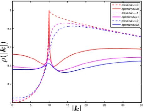
A numerical example of the convergence factor is shown in Figure 1. We can see that for σ > 0, the classical Schwarz algorithm does not have convergence problems any more close to the resonance frequency. Increasing σ further improves the performance, since the maximum of the convergence factor de-creases. We also see that the optimization, which is based on equioscillation, leads to a uniformly small contraction factor when σ > 0, whereas in the case σ = 0 a small region close to the resonance frequency needs to be excluded in order to minimized the convergence factor for the remaining frequencies.
0 5 10 15 20 25 30 35 0 0.2 0.4 0.6 0.8 1 classical !=0 optimized!=0 classical !=1 optimized!=1 classical !=2 optimized!=2 ρ (| k| ) |k|
6 V. Dolean et al.
4 Numerical Results
We present now some numerical tests in order to illustrate the performance of the algorithms. The domain Ω is partitioned into several subdomains Ωj.
In each subdomain, we use a discontinuous Galerkin method (DG), see [5]. We first test the propagation of a plane wave in a homogeneous medium. The domain is Ω = (0, 1)2, and the parameters are constant in Ω, with
ε = µ = 1, σ = 5 and ω = 2π. We impose on the boundary an incident field Winc = (Hinc
x , Hyinc, Ezinc) = ( ky
µω,−k
x
µω , 1)e−ik·x with k = (kx, ky) =
(ω"ε− iσ
ω, 0), x = (x, y). The domain Ω is decomposed into two
subdo-mains Ω1= (0, 1/2) × (0, 1) and Ω2= (1/2, 1) × (0, 1). For this test case, the
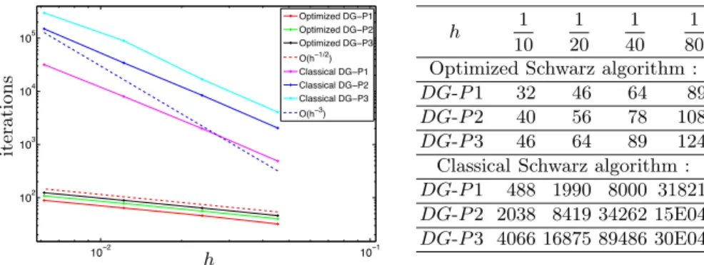
DG method is used with a uniform polynomial approximation of order one, two and three, denoted by DG-P 1, DG-P 2 and DG-P 3. The performance of the algorithm is shown in Figure 2. These results are in good agreement with
10−2 10−1 102 103 104 105 Optimized DG−P1 Optimized DG−P2 Optimized DG−P3 O(h−1/2) Classical DG−P1 Classical DG−P2 Classical DG−P3 O(h−3) it er a ti o n s h h 1 10 1 20 1 40 1 80 Optimized Schwarz algorithm :
DG-P 1 32 46 64 89
DG-P 2 40 56 78 108
DG-P 3 46 64 89 124
Classical Schwarz algorithm :
DG-P 1 488 1990 8000 31821
DG-P 2 2038 8419 34262 15E04 DG-P 3 4066 16875 89486 30E04
Fig. 2. Number of iterations against the mesh size h, to attain a relative residual
reduction of 10−8 obtained with the classical and optimized Schwarz algorithm
the theoretical result in Theorem 3: the curves fit nicely the dependence on h predicted, i.e they behave like h−0.5. We also see the tremendous
improve-ment of the optimized Schwarz method over the classical Schwarz method, which nevertheless performs a bit better than predicted in Corollary 1, the dependence on h measured is O(h−2), instead of O(h−3); for an explanation,
see [7].
The second test problem is a simplified model of the propagation of an electromagnetic wave, emitted by a localized source, in the head tissues. The geometric configuration is given in Figure 3. The electromagnetic parameters of the material in the head tissues are: µ = 1 in the whole domain, ε = 43.85, σ = 1.23· 120π for the skin, ε = 15.56, σ = 0.43 · 120π for the skull, ε = 67.20, σ = 2.92· 120π for the cerebrospinal fluid and ε = 43.55, σ = 1.15 · 120π for the brain. The antenna is modeled by two perfectly conducting rods (with base section of 0.252cm2) and between these rods a current density J
Skin Skull Cerebrospinal fluid Brain 12cm 10cm 10.5cm 8.3cm X Y Source
Fig. 3. Model of the different layers of a skull
-0.2 -0.15 -0.1 -0.05 0 0.05 0.1 0.15 0.2 -0.2 -0.15 -0.1 -0.05 0 0.05 0.1 0.15 0.2 x y
Fig. 4. Decomposition into subdomains and solution
applied. The computational domain is decomposed into several subdomains (a decomposition into eight subdomains is shown for example in Figure 4 on the left). We compare in this test the performance of the classical Schwarz and the new optimized Schwarz algorithm for a decomposition into two, four, eight and sixteen subdmains. In Table 1, we show the number of iterations needed for convergence, i.e to attain a relative residual of 10−8, depending on
the number of subdomains. These results show that the optimized Schwarz algorithm converges much faster than the classical Schwarz algorithm. Here we used a Krylov method (BiCGStab) for the solution of the linear system, preconditioned with the classical and optimized Schwarz preconditioner.
Number of subdomains 2 4 8 16
Classical Schwarz 94 197 179 174
Optimized Schwarz 69 92 82 85
8 V. Dolean et al.
5 Conclusion
We analyzed an optimized Schwarz method for the two dimensional Maxwell equations with non-zero electric conductivity. The new method performs much better than the classical one, and our theoretical results are well confirmed by the numerical experiments presented, also for a non-trivial test case.
References
[1] A. Alonso-Rodriguez and L. GerarGiorda. New nonoverlapping do-main decomposition methods for the harmonic Maxwell system. SIAM J. Sci. Comput., 28(1):102–122, 2006.
[2] P. Chevalier and F. Nataf. An OO2 (Optimized Order 2) method for the Helmholtz and Maxwell equations. In 10th International Conference on Domain Decomposition Methods in Science and in Engineering, pages 400–407. AMS, 1997.
[3] B. Despr´es. D´ecomposition de domaine et probl`eme de Helmholtz. C.R. Acad. Sci. Paris, 1(6):313–316, 1990.
[4] B. Despr´es, P. Joly, and J.E. Roberts. A domain decomposition method for the harmonic Maxwell equations. In Iterative methods in linear alge-bra, pages 475–484, Amsterdam, 1992. North-Holland.
[5] V. Dolean, M. El Bouajaji, M.J. Gander, S. Lanteri, and R. Perrussel. Domain decomposition methods for electromagnetic wave propagation problems in heterogeneous media and complex domains. In Domain De-composition Methods in Science and Engineering XIX, 2010. submitted. [6] V. Dolean and M.J. Gander. Why classical schwarz methods applied to hyperbolic systems can converge even without overlap. In Domain Decomposition Methods in Science and Engineering XVIII, pages 467– 476. Springer Verlag, 2007.
[7] V. Dolean and M.J. Gander. Can the discretization modify the per-formance of schwarz methods? In Domain Decomposition Methods in Science and Engineering XIX, 2010. submitted.
[8] V. Dolean, L. Gerardo-Giorda, and M.J. Gander. Optimized Schwarz methods for Maxwell equations. SIAM J. Scient. Comp., 31(3):2193– 2213, 2009.
[9] V. Dolean, S. Lanteri, and R. Perrussel. A domain decomposition method for solving the three-dimensional time-harmonic Maxwell equa-tions discretized by discontinuous Galerkin methods. J. Comput. Phys., 227(3):2044–2072, 2008.
[10] V. Dolean, S. Lanteri, and R. Perrussel. Optimized Schwarz algorithms for solving time-harmonic Maxwell’s equations discretized by a discon-tinuous Galerkin method. IEEE. Trans. Magn., 44(6):954–957, 2008. [11] M.J. Gander, F. Magoul`es, and F. Nataf. Optimized Schwarz methods
without overlap for the Helmholtz equation. SIAM J. Sci. Comput., 24(1):38–60, 2002.

![[PDF] Formation développement d’applications avec les bases de données PL/SQL | Cours informatique](data:image/gif;base64,R0lGODlhAQABAIAAAP///wAAACH5BAEAAAAALAAAAAABAAEAAAICRAEAOw==)