A validation of heat and carbon fluxes from high-resolution land surface and regional models

HAL Id: hal-01136713

https://hal.archives-ouvertes.fr/hal-01136713

Submitted on 27 Mar 2015

HAL is a multi-disciplinary open access

archive for the deposit and dissemination of

sci-entific research documents, whether they are

pub-lished or not. The documents may come from

teaching and research institutions in France or

abroad, or from public or private research centers.

L’archive ouverte pluridisciplinaire HAL, est

destinée au dépôt et à la diffusion de documents

scientifiques de niveau recherche, publiés ou non,

émanant des établissements d’enseignement et de

recherche français ou étrangers, des laboratoires

publics ou privés.

high-resolution land surface and regional models

A. Anav, F. d’Andrea, N. Viovy, N. Vuichard

To cite this version:

A. Anav, F. d’Andrea, N. Viovy, N. Vuichard. A validation of heat and carbon fluxes from

high-resolution land surface and regional models. Journal of Geophysical Research: Biogeosciences,

Amer-ican Geophysical Union, 2010, 115 (4), pp.G04016. �10.1029/2009JG001178�. �hal-01136713�

A validation of heat and carbon fluxes from high

‐resolution land

surface and regional models

Alessandro Anav,

Fabio D

’Andrea,

Nicolas Viovy,

and Nicolas Vuichard

Received 16 October 2009; revised 22 May 2010; accepted 26 July 2010; published 5 November 2010.

[1]

The performance of Organizing Carbon and Hydrology in Dynamic Ecosystems

(ORCHIDEE), a model of surface hydrology, plant phenology, and vegetation dynamics,

in reproducing field measurements of heat and carbon fluxes at various spatial and

temporal scales is assessed. The model is forced by two high

‐resolution (30 km) regional

climate models (RegCM3 and WRF) output in the Euro

‐Mediterranean region for the

period 2002–2007. First a validation of the regional models surface climatology is

conducted in comparison to gridded meteorological station data and to other state of the art

regional models. Then annual cycles and interannual variability of latent and sensible heat,

gross primary production, and net ecosystem exchange are compared to in situ

experimental data provided from the CARBOEUROPE network. Six sites were chosen

across the Euro

‐Mediterranean region, representing different forest environments. Results

show that ORCHIDEE is able to reproduce the annual cycle of heat and carbon fluxes,

with errors comparable with the measurement uncertainties. The interannual variations

appear more problematic. While the variations of sensible heat are at least of the same sign

as observed, latent heat is less well reproduced, while there is hardly any skill in

reproducing carbon fluxes. The main difference between the two regional models used for

forcing is an excessive precipitation produced on average by RegCM3. This causes errors

in the latent heat and gross primary production of ORCHIDEE.

Citation: Anav, A., F. D’Andrea, N. Viovy, and N. Vuichard (2010), A validation of heat and carbon fluxes from high‐resolution land surface and regional models, J. Geophys. Res., 115, G04016, doi:10.1029/2009JG001178.

1.

Introduction

[2] The land surface plays a pivotal role in the Earth

system through physical, biophysical and biogeochemical interaction with the atmosphere and oceans [Foley et al., 1994; Prentice et al., 2000]. Land‐atmosphere interac-tions include complex feedbacks between soil, vegetation, and atmosphere through the exchanges of water, momen-tum, energy and greenhouse gases [Pielke et al., 1998; Arora, 2002]. Each feedback has a great importance at different timescales from medium range weather prediction to climate variability and change [Pielke et al., 1998]. Reasonable estimate of the mean state of the atmosphere is indispensable to correctly represent these feedbacks in general circulation models (GCMs) or regional climate models (RCMs) [Alessandri et al., 2007; Steiner et al., 2009].

[3] Surface‐vegetation‐atmosphere transfer schemes

(SVATs) are used in GCMs and RCMs to simulate exchanges of sensible and latent heat, of kinetic energy at the surface, as well as of water mass [Calvet et al., 1998;

Gibelin et al., 2006; Alessandri et al., 2007; Jarlan et al., 2008; Steiner et al., 2009]. However, the SVAT models are in general not able to simulate the transient structural changes of vegetation cover in response to climatic changes by explicitly modeling species competition and dis-turbances [Arora, 2002]. Moreover, the SVAT models do not account for the role of terrestrial vegetation in the carbon cycle variability [Alessandri et al., 2007]. Finally, the absence of dynamic vegetation in the SVAT schemes implies that the effect of climate variability in modifying physiological characteristics of vegetation is not taken into account [Arora, 2002]. Too little or too much precipitation, for example, is assumed to make no difference in plant productivity and resulting Leaf Area Index (LAI) [Arora, 2002].

[4] To overcome these problems, Dynamic Global

Vege-tation Models (DGVMs) [e.g., Foley et al., 1996; Sitch et al., 2003; Krinner et al., 2005] have been developed to be coupled to climate models [Foley et al., 1998; Bonan et al., 2002, 2003], both global and regional.

[5] The aim of this paper is to evaluate the ability of

ORCHIDEE [Krinner et al., 2005], a model of surface hydrology, plant phenology and vegetation dynamics, to reproduce field measurements of heat and carbon fluxes at different spatial and temporal scales, when it is forced with high‐resolution (30 km) RCMs outputs for Euro‐ Mediterranean region.

1

Laboratoire de Meteorologie Dynamique, IPSL, École Normale Supérieure, Paris, France.

2_{Laboratoire des Sciences du Climat et de l’Environnement, Gif‐}

sur‐Yvette, France.

Copyright 2010 by the American Geophysical Union. 0148‐0227/10/2009JG001178

[6] DGVMs, including ORCHIDEE, have been

exten-sively used at global scale to account the global terrestrial carbon cycle [Krinner et al., 2005], and have already been used at the local scale [Morales et al., 2005; Santaren et al., 2007; Keenan et al., 2009; Mahecha et al., 2010]. The local‐ scale validation [e.g., Morales et al., 2005], uses comparison with measurements obtained at flux tower sites [e.g., Baldocchi et al., 2001] and is often limited to the annual timescale, checking the seasonal cycle of fluxes and the timing of the growing season [Morales et al., 2005; Mahecha et al., 2010]. In general off‐the‐shelf DGVMs perform poorly at the local level unless parameters are cal-ibrated for the given site, e.g., by parameter inversion [Santaren et al., 2007].

[7] Only few works exist [e.g., Jung et al., 2007; Vetter

et al., 2008], that use regional climate models (RCMs) as forcing for DGVMs. Nevertheless, RCMs provide an increase in resolution and can capture physical processes and feedbacks occurring at the regional scale [Morales et al., 2007]; this would allow the DGVMs to capture physical and ecological processes at finer resolution that could influence the carbon cycle [Morales et al., 2007]. Changes in model vegetation patterns with associated changes in carbon fluxes and storage can be expected as a consequence of increased resolution. In fact, DGVM are highly sensitive to fine‐scale climate variations, especially in regions of com-plex topography and surface cover (e.g., the Alps, the Mediterranean or Scandinavia), and in areas with strong maritime influence (e.g., around the Baltic Sea). Therefore, if there is a need to assess the carbon cycle at a regional scale, then the coarse resolution of GCM is a serious limitation [Morales et al., 2007].

[8] Given the considerations above, the goal of this paper

is to assess the performance of the specific DGVM, namely ORCHIDEE, using high‐resolution forcing, issued by regional climate models. We performed a severe validation of the model, at different spatial scales, distinguishing between intraseasonal and interannual variations. Specifi-cally, we address the following questions: is ORCHIDEE able to correctly simulate the mean annual cycle of heat and carbon fluxes? Is it able to capture the interannual variability of these fluxes?

[9] The paper is organized as follows. The models and

the experimental setup are described with some detail in section 2, while the results are presented in section 3. Specifically, section 3.1 contains a validation of the regional model integrations with respect to the CRU [New et al., 2002] observed data. The goal of this section is to be sure that, before forcing ORCHIDEE, the RCMs out-puts correctly reproduce at least the observed 2 m air temperature and precipitation. We also checked if the regional simulation results have comparable performances to other high‐resolution regional models; the models par-ticipating to the PRUDENCE project [Jacob et al., 2007] are used as reference. The integration period chosen in this study, however, goes beyond the reference period of PRUDENCE, and has the particular interest of including two extreme climatologic events that took place in the region, namely the heat wave of summer 2003 and the anomalously hot winter of 2007.

[10] Section 3.2 presents a comparison of the ORCHIDEE

heat and carbon fluxes against observed CARBOEUROPE

(http://www.carboeurope.org/) data at some European locations. The comparison includes also the fluxes predicted by the regional atmospheric models themselves via their SVAT modules. The station sites were chosen at six Euro-pean locations corresponding to different forest ecosystems; in these sites, we compare the simulated water and carbon fluxes with data obtained from measurement towers [Aubinet et al., 2000; Baldocchi et al., 2001; Falge et al., 2001; Friend et al., 2007; Reichstein et al., 2005; Papale et al., 2006]. Finally, discussions and conclusions are pro-vided in section 4.

2.

Models Description and Experiments

[11] Two mesoscale models (RegCM3 and WRF3) have

been integrated to simulate the present‐day hydro‐climate for the Euro‐Mediterranean basin. The simulations cover the period 2002–2007. In the experimental setup we used the same model resolution and domain as well as the same large scale forcing, so that the influence of factors specific to the internal model physics and dynamics can be determined.

[12] The models domain is centered at 41°N and 15°W

and is projected on a normal Mercator grid covering almost all Europe (except northern Scandinavia and Iceland) and North Africa. The domain covers 190 × 190 grid points in the longitudinal and latitudinal directions, respectively, with a horizontal resolution of 30 km. The model domain is shown in Figure 1.

[13] The larger model boundary conditions required to run

the mesoscale models were provided by the National Center for Environmental Prediction/National Center for Atmo-spheric Research Reanalysis Project (NNRP) data. The NCAR‐NCEP reanalysis have a resolution of 2.5 × 2.5 degrees and have been interpolated into the models domain to produce initial and lateral boundary conditions.

[14] The models are briefly described here with a focus on

the main differences between RegCM3 [Pal et al., 2007, and references therein] and WRF [Skamarock et al., 2005]. RegCM3 is a limited area model initially developed by Giorgi [1990] and Giorgi et al. [1993a, 1993b] and then modified as discussed by Giorgi and Mearns [1999] and Pal et al. [2000, 2007]. The model is a primitive equation, hydrostatic, and compressible that employs a terrain fol-lowings‐vertical coordinate. In the present work we set 18 sigma levels with the top at 50 hPa.

[15] The RegCM3 includes different physics options [Pal

et al., 2007]. The dynamical core of the RegCM3 is essen-tially equivalent to the hydrostatic version of the NCAR/ Pennsylvania State University mesoscale model MM5 [Grell et al., 1994]. The atmospheric radiative transfer computations are performed using the CCM3‐based package [Kiehl et al., 1996] and the planetary boundary layer computations are performed using the nonlocal formulation of Holtslag et al. [1990]. Resolvable scale precipitation is represented via the scheme of Pal et al. [2000] which includes a prognostic equation for cloud water and allows for fractional grid box cloudiness, accretion and reevaporation of falling precip-itation. Convective precipitation is represented using the cumulus convection scheme of Grell [1993] with the Fritsch and Chappell [1980] closure assumption. Air‐sea

exchanges are treated using the parameterization of Zeng et al. [1998].

[16] Generally, the main difference in surface climate

between different RCMs are determined by the land surface parameterization. The heat, water and momentum exchanges between the land surface and the boundary layer is simu-lated in RegCM3 by the hydrological process model BATS (Biosphere–Atmosphere Transfer Scheme) [Dickinson et al., 1993]. The model has a vegetation layer, a snow layer, a surface soil layer (10 cm thick), a root zone layer (1–2 m thick) and a deep soil layer (3 m thick). BATS divides the land surface into 18 types and the soil in 12 types [Dickinson et al., 1993]. These 18 classes of land cover are used to define a wide variety of land surface, hydrological and vegetation properties: each vegetation class, in fact, has associated a value of roughness length, albedo, LAI, rooting depth and the fraction of water extracted by the roots [Dickinson et al., 1993].

[17] The Weather Research and Forecasting (WRF) model

is a fully compressible and nonhydrostatic model (with a runtime hydrostatic option), and it represents an evolution of the MM5 model. It uses s‐vertical coordinate, and in the present work we set 27 sigma levels with the top at 50 hPa. [18] The WRF model system also offers multiple options

for various physical packages [Skamarock et al., 2005]. The WRF dynamical core used in this work is ARW [Skamarock et al., 2005], with a single‐moment 3‐class scheme to

resolve the microphysics, the rapid radiative transfer model (RRTM) for the longwave radiation [Mlawer et al., 1997], and the Dudhia scheme for the shortwave radiation [Dudhia, 1989]. Convective precipitation and cumulus parameteriza-tion are resolved via the Grell scheme [Skamarock et al., 2005], and the planetary boundary layer computations are performed using the Yongsei University parameterization [Noh et al., 2003].

[19] The exchange of heat, water and momentum between

soil‐vegetation and atmosphere is simulated by the NOAH Land Surface Model [Skamarock et al., 2005]. The NOAH model contains four soil layers: a thin 10 cm top layer, a second root zone layer of 20 cm, a deep root zone layer of 60 cm, and a subroot zone layer of 110 cm. It has 13 veg-etation covers and nine different soil types [Hogue et al., 2005]. The NOAH provides sensible and latent heat fluxes to the boundary layer scheme. The NOAH LSM additionally predicts soil ice, and fractional snow cover effects, has an improved urban treatment, and considers surface emissivity properties, which are all new since the OSU scheme [Skamarock et al., 2005]. Vegetation dynamics are not explicitly modeled by any of the two models.

2.2. Biogeochemical Flux Model

[20] The temperature, precipitation, specific humidity,

wind speed, pressure, short wave and long wave incoming Figure 1. Model domain with the corresponding topography (units are in meters). The PRUDENCE

subdomains where some of the model diagnostics have been computed are also shown (see text for details).

ANAV ET AL.: VALIDATION OF HEAT AND CARBON FLUXES G04016 G04016

radiation simulated by RegCM3 and WRF models have been used to run the land surface model ORCHIDEE (Organizing Carbon and Hydrology in Dynamic Ecosys-tems). ORCHIDEE is a SVAT model coupled to a bio-geochemistry and a dynamic biogeography model [Krinner et al., 2005]. Specifically, ORCHIDEE simulates the fast feedbacks occurring between the vegetated land surface and the atmosphere, the terrestrial carbon cycle, and changes in vegetation composition and distribution in response to climate change.

[21] ORCHIDEE is based on three different modules

[Krinner et al., 2005]. The first module, called SECHIBA [Ducoudré et al., 1993], describes the fast processes such as exchanges of energy and water between atmosphere and biosphere, and soil water budget. It has a 30 min time step. SECHIBA has two soil layers of variable depths. The total depth of the soil is 2 m and it is constant throughout the continents. The storage capacity is a function of the land cover types. In vegetation‐covered areas the storage capacity is prescribed as 150 mm water for each meter of soil depth, while bare soils have a reduced water storage capacity of 30 mm for each meter of soil depth [Alessandri et al., 2007]. The current soil texture map is based on Zobler [1986]; further details about the parameterizations of soil hydrology and turbulent fluxes are given by Ducoudré et al. [1993], De Rosnay and Polcher [1998], and D’Orgeval et al. [2008].

[22] The phenology and carbon dynamics of the terrestrial

biosphere are simulated by STOMATE (Saclay Toulouse Orsay Model for the Analysis of Terrestrial Ecosystems) model [Krinner et al., 2005]. Specifically, STOMATE si-mulates processes as photosynthesis, carbon allocation, litter decomposition, soil carbon dynamics, maintenance and growth respiration, and phenology on a daily time step. Photosynthesis is based on the Farquhar et al. [1980] model for C3 plants and of Collatz et al. [1992] for C4 plants. Maintenance respiration is a function of each liv-ing biomass pool and temperature. Growth respiration is computed as a fraction of the difference between assim-ilation inputs and maintenance respiration outputs to plant biomass. Heterotrophic respiration parameterization is taken from the CENTURY model [Parton et al., 1988]. Carbon dynamics are described through the exchanges of carbon between the atmosphere and the different carbon pools in plants and soils. ORCHIDEE has eight biomass pools, four litter pools, and three soil carbon pools; fur-ther details are given by Krinner et al. [2005]. Turnover time for each of the soil carbon and litter pools depends mainly on temperature and humidity. The parameteriza-tions of litter decomposition and soil carbon dynamics essentially follow Parton et al. [1988]. For any given PFT (Plant Functional Type), several parameters are provided in

order to account all the different processes simulated by ORCHIDEE. These parameters have been estimated in laboratories or at spatial scales of centimeters to meters in the field [Farquhar et al., 1980; Lloyd and Taylor, 1994; Sitch et al., 2003; Krinner et al., 2005].

[23] Long‐term processes (on yearly time step), including

vegetation dynamics, fire, sapling establishment, light competition, and tree mortality are simulated according to the global vegetation model LPJ [Sitch et al., 2003]. For any grid point, a mosaic of different vegetation types can coexist and compete for resources. ORCHIDEE distin-guishes 12 PFTs (of which 10 are natural and two agricul-tural) [Krinner et al., 2005]. The fraction of the element occupied by each PFT is either calculated (and thus variable in time) or prescribed when LPJ is deactivated.

[24] In the following, ORCHIDEE is forced by hourly data

provided by RCMs models output in the explicit DGVM mode (LPJ active) [Krinner et al., 2005]. In order to initialize plant distribution and soil carbon a 400 years spin‐up have been performed using preindustrial CO2levels. At the end of spin‐up, we performed the simulation for years 2002–2007 using the measured annual atmospheric CO2concentration.

[25] In order to avoid that poor model performances could

be related to the bad quality of forcing data provided by mesoscale models, we also ran ORCHIDEE at six stand sites using the half‐hourly forcing provided by CARBOEUROPE measurements (discussed later). In such case, the vegetation is prescribed according to the observed dominant vegetation cover (Table 1) and LPJ is deactivated, hence vegetation dynamic and competition among PFTs are not taken into account.

2.3. Measurements and Sites Description

[26] In order to analyze their ability to simulate 2 m air

temperature and precipitation, the two regional models are validated against the observed CRU [New et al., 1999, 2000, 2002] data set. This data set consists of gridded data ob-tained from a collection of meteorological stations, which were quality controlled and aggregated at a resolution of 0.5 degree.

[27] For this analysis, the data were further aggregated on

eight subdomains (Figure 1) over the European region. These subdomains are the standard ones that were employed for model diagnostics in the regional climate change project PRUDENCE [Christensen and Christensen, 2007].

[28] For this validation, initially we used the European

Climate Assessment (ECA) data set [Klein Tank et al., 2002] instead of CRU. We found a mismatch in the tem-perature bias sign with respect to other published model intercomparisons [Jacob et al., 2007]. More precisely, we found a positive bias when we compared simulated tem-perature against ECA, while Jacob et al. [2007] generally

Table 1. Main Characteristics of the Six Sites Used for Model Validation: Dominant Species, Climatic Features, and Leaf Area Index Site Name Dominant Species Mean Annual Temperature (°C) Precipitation (mm/yr) Elevation (m) LAI Reference Hainich Fagus sylvatica 7 750 445 6 Knohl et al. [2003] Sorø Fagus sylvatica 8.1 510 40 4.8 Pilegaard et al. [2001] Hesse Fagus sylvatica 9.2 885 300 7.6 Granier et al. [2000] Loobos Pinus sylvestris 9.8 786 52 2.2 Dolman et al. [2002] Tharandt Picea abies 7.5 820 380 7.6 Bernhofer et al. [2003] Puechabon Quercus ilex 13.5 883 270 2.9 Rambal et al. [2003]

show a cold bias of most models against CRU data. In fact, we could verify that a mean temperature difference of around 2 degrees is found between the two observational data sets. Therefore, we chose to perform the model vali-dation only with respect to CRU in order to be consistent with previous works done in the framework of the PRUDENCE project. We are not aware, in literature, of any work comparing the two data sets.

[29] After the analysis of temperature and precipitation,

the validation is focused on heat and carbon fluxes as reproduced by the ORCHIDEE model forced off‐line by the two models output. The intercomparison of heat fluxes can be extended to the fluxes computed by the land surface schemes of the two mesoscale models.

[30] Under the auspices of the CarboEurope‐IP an

extensive set of eddy covariance flux measurement towers has been established all over Europe, supporting ecosystem level research on energy and mass transfer processes [Aubinet et al., 2000]. Hence, the ecosystem–atmosphere CO2and H2O exchange data, used for the model validation,

have been collected at different sites (Table 1) within the CARBOEUROPE ecosystem flux component. The choice of these specific sites is due to the multiple requirements of having a long enough data coverage, and of representing typical natural vegetation in Europe. Specifically, the sites refer to different plant types covering the most important European forest ecosystems: temperate deciduous (Hesse, Sorø, Hainich), temperate coniferous (Tharandt, Loobos), and Mediterranean (Puechabon). These sites have experi-enced varying disturbance histories, management practices, and are also situated in different climate conditions of mean temperature, precipitation. The main characteristics of the sites and references providing each site description are given in Table 1.

3.

Results

3.1. Validation of Temperature and Precipitation [31] Estimates of the 2 m temperature models biases are

shown in Figure 2 for the four seasons and for the eight Figure 2. Seasonal mean (2002–2006) values of observed (CRU, blue), reanalyzed (NCEP, black), and

simulated (RegCM3, red, WRF, green) 2 m temperature over the eight European PRUDENCE subregions with the associated standard deviations. Only the land data are included in the regional average. (top to bottom) Winter, spring, summer, and fall.

ANAV ET AL.: VALIDATION OF HEAT AND CARBON FLUXES G04016 G04016

PRUDENCE domains [Christensen and Christensen, 2007]. In Figure 2 the seasonal means and standard deviations (computed on the year‐to‐year variations) simulated by RegCM3 and WRF are compared to CRU data. The averages and standard deviations are computed on the period 2002–2006 and only for land points.

[32] In general, both RegCM3 and WRF models tend to

slightly underestimate temperature (Figure 2). The tem-perature bias (RMSE) of RegCM3 is 0.1 to more than 1 degree smaller than that of WRF, except in summer when WRF is actually better (Table 2). These differences,

however, do not pass a 95% test of significance, except in the SON season.

[33] The larger differences between RegCM3 and CRU

data occur in JJA (Table 2), mainly in the Mediterranean (MD, 2.5°C), Alps (AL, 2.5°C), Iberian Peninsula (IP, 2°C), and France (FR, 2°C) subdomains (Figure 2), while the bias has minimum levels during DJF and SON (Table 2). As for WRF, the higher bias is in SON (Table 2) where it is con-stantly above 2°C in all subdomain and in the case of Mediterranean region it reaches 5°C.

[34] A temperature bias with the same sign is also found

comparing CRU and NCEP data, as shown in the last col-umn of Table 2 (see also Figure 2). Consequently the error appears to be introduced in the regional models integrations by the boundary forcing. The downscaling by the regional models does reduce this error, except in summer, but it re-mains considerable. It is also noteworthy that only the NCEP temperature has been used to force the mesoscale models, while precipitation is diagnostically computed by both models.

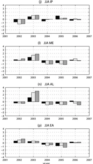
[35] The interannual variations of the observed and

sim-ulated temperature for summer and winter in the eight PRUDENCE domains can be seen in Figure 3, where the

Table 2. Temperature and Precipitation RMS Errors for RegCM3, WRF, and the NCEP Reanalysis, With Respect to the CRU Gridded Data

Variable Model DJF MAM JJA SON 2 m temperature (°C) RegCM3 1.3 1.4 1.8 1.6 WRF 2.1 1.8 1.7 3.0 NCEP 2.6 1.7 1.2 1.6 Precipitation (mm/d) RegCM3 0.9 1.3 1.5 0.7 WRF 0.8 0.3 1.0 0.8 NCEP 1.0 0.8 0.9 1.2

temperature anomaly for each year is shown with respect to seasonal climatology. As for the seasonal mean temperature (Table 3), RegCM3 captures somewhat better the interannual variability. The sign of the interannual variations is generally captured by both models; it is noteworthy for example the strong hot signal relative to the 2003 summer heat wave in central Europe (Figures 3k and 3l and Figures 3n and 3o). The RMS error in the amplitude of the variability is slightly higher on average for WRF (0.44°C) than for RegCM3 (0.39°C) but the difference is not statistically significant according to a confidence level of 95%. In some seasons and domains WRF has a better performance, for example in the Iberian Peninsula during all the seasons, but this remains only marginally significant. Also for the interannual vari-ability, WRF simulates somewhat better the summer season than RegCM3 (0.37°C, 0.44°C, respectively).

[36] Estimates of precipitation biases are shown in

Figure 4 for the four seasons and the different domains. The bias (RMSE) goes from 1.1 mm/d for RegCM3 to 0.8 mm/d for WRF, on average for the whole year and all the domains and the differences are significant with 99% confidence level. The scores divided by seasons are reported in Table 2.

[37] In the case of RegCM3, the larger bias occurs during

summer (Table 2), mainly in the Scandinavian region (SC, 2.5 mm/d) and in France (1.8 mm/d, Figure 4), while the bias has a minimum level during SON; in this season RegCM3 simulate precipitation slightly better than WRF (Table 2). The positive bias in RegCM3 precipitation over land has been already described in the standalone [Giorgi et al., 2004] and in the coupled [Artale et al., 2009] RegCM3 versions.

[38] In WRF the highest bias occurs during summer; in

such season the model systematically underestimates the land precipitation in all subdomains (Figure 4). The regions with the larger error are AL (1.7 mm/d), SC (1.4 mm/d), and

Table 3. RegCM3 and WRF Interannual Variability RMS Errors for Temperature and Precipitation

Variable Model DJF MAM JJA SON 2 m temperature (°C) RegCM3 0.35 0.27 0.44 0.45 WRF 0.53 0.33 0.37 0.5 Precipitation (mm/d) RegCM3 0.3 0.25 0.38 0.43

WRF 0.78 0.16 0.21 0.22

Figure 3. (continued)

ANAV ET AL.: VALIDATION OF HEAT AND CARBON FLUXES G04016 G04016

BI (1 mm/d), while the others domains have errors lower than 1 mm/d.

[39] The interannual variability of precipitation offers a

more complex picture than temperature. At places and times the models do not even get the sign of the vari-ability right (Figure 5). More precisely in DJF WRF has a very poor behavior representing the interannual vari-ability (0.78 mm/d), while RegCM3 (0.3 mm/d) generally has the same sign of CRU (Figure 5). During JJA the bias is smaller for both models, as reported in Table 3.

[40] RegCM3 has thus more realistic interannual

vari-ability in winter, despite the higher seasonal bias. In the other seasons, WRF is better and the differences are sig-nificant with a confidence level of 95%. These results for RegCM3 temperature and precipitation are in accordance to the bias found in the regional climate model intercompari-son [Jacob et al., 2007] although the time period is different. [41] While the above analysis against CRU data is

reassur-ing as far as the general performance of the models is concerned, the consistency of the above diagnostics has to be checked with respect to the CARBOEUROPE station data that can be affected by local features. This check has been

carried out (not shown), and results generally agree with the validation performed on the subbasins.

3.2. Validation Against Stand Site Data 3.2.1. Heat Fluxes

[42] In Figure 6, the 6 year averaged annual cycle of latent

heat flux is shown for ORCHIDEE forced by the two regional models (light and dark blue lines) and for the ref-erence CARBOEUROPE data (black asterisks). The analy-sis is conducted for the six chosen CARBOEUROPE stations. In Figure 6, also the heat fluxes directly computed by the regional models and their own SVAT scheme is plotted (red and green lines). These last two lines are added for completeness; it should be reminded however that the SVAT schemes of the two regional models are fully coupled with the atmospheric part of the models, and therefore they take into account feedbacks, while ORCHIDEE is forced offline. Finally, results of ORCHIDEE forced directly by the meteorological variables measured in the CARBOEUROPE stations are shown as black lines.

[43] In general terms, ORCHIDEE reproduces reasonably

well the mean annual cycle of latent heat flux when forced Figure 4. As Figure 2 but for precipitation.

by RegCM3 and WRF (Figure 6); the differences between these two ORCHIDEE simulations are weak and not sig-nificant. The mean bias with respect to CARBOEUROPE data ranges around 20 W/m2 when ORCHIDEE is forced with RegCM3 (henceforth ORC‐REG) and 19 W/m2

when forced with WRF (henceforth ORC‐WRF). In most panels of Figure 6, ORCHIDEE slightly overestimates the latent heat flux; the looser performances of ORCHIDEE occur in FR‐PUE (south of France) for both ORC‐REG (31 W/m2) and ORC‐WRF (23 W/m2

).

[44] Taking into account the RCMs performances,

RegCM3, with BATS, overestimates latent heat in all sites (Figure 6) more severely; this strong positive bias is in agreement with the excess in precipitation that generate a high amount of water in the soil, (see Figure 4). The mean bias (44 W/m2) is twice as high as that of ORCHIDEE.

[45] It is noteworthy that when ORCHIDEE is driven by

RegCM3, it does not show the same overestimation of latent heat, and the flux has the same magnitude of the ORC‐WRF. In the case of ORC‐REG, the excess precip-itation does not evaporate but increases soil moisture (20% more in ORC‐REG with respect to ORC‐WRF).

[46] The bias of WRF coupled with NOAH is the lowest

compared to the other models, about 16 W/m2. Finally, forcing ORCHIDEE with the station data (henceforth ORC‐CEIP) gives the best results; in this case the bias is about 14 W/m2 and results are statistically indistinguish-able form the observations.

[47] Considering that the uncertainties in the station

mea-surements are of the order of 20 W/m2[Hollinger and Richardson, 2005] all these biases, with the possible exception of RegCM‐BATS should be considered quite low. [48] Despite ORCHIDEE replicated the seasonal patterns

of latent heat reasonably well, in some sites the model performances are poor. In particular, in FR‐PUE the sum-mer stomatal closure related to the high soil moisture stress is not captured by any simulation, except ORC‐WRF. In the case of ORC‐REG, the excess of precipitation does not produce any severe summer drought, hence this result is not unexpected; however, also ORC‐CEIP had difficulty trying to match the observed trend of latent heat flux.

[49] Figure 7 shows the interannual variability of latent

heat for JJA. Only summer is shown in Figure 7and in the following showing sensible heat and carbon fluxes, because Figure 5. As Figure 3 but for precipitation.

ANAV ET AL.: VALIDATION OF HEAT AND CARBON FLUXES G04016 G04016

the main activities of vegetation are concentrated in this season, as well as its interaction mechanisms with climate. The one exception is for FR‐PUE; since the period of main activity of vegetation in this site is in spring (see Figure 10), we concentrate on MAM in all further analysis.

[50] The comparison of simulated interannual variations of

latent heat with station data reveals a complex pattern with strong and statistically significant discrepancies. Model per-formances are quite poor, particularly in DK‐SOR, NL‐LOO, DE‐THA, and FR‐PUE. Overall, between the five simula-tions, WRF is the model that better reproduces the interannual variability both in JJA and during the whole year (not shown). The overall RMS error computed taking into account all the seasons is about 6 W/m2for WRF, 7 W/m2for RegCM3, and 7 W/m2 and 8 W/m2 for ORC‐REG and ORC‐WRF, respectively. Forcing ORCHIDEE with site measurements gives a little improvement in performance with respect to ORCHIDEE forced by the regional models. The overall bias, for all seasons and sites, is 6 W/m2. This result is also far from perfect, considering that the natural variability (stan-dard deviation at the interannual timescale) is approximately 5 W/m2.

[51] Looking at sensible heat mean annual cycle (Figure 8)

all the models are in the same range (except in FR‐PUE), and they generally match the observations. Because of the over-estimation of latent heat, RegCM3 has lower levels of sen-sible heat. Even if the biases are quite close to one another, the differences are significant, but, as in the case of latent heat, they remain in the order of magnitude of the measurement uncertainties. ORC‐WRF has the lower bias (19 W/m2), while ORC‐CEIP has highest (26 W/m2

). Considering this latter simulation, ORC‐CEIP is not able to correctly reproduce the seasonal cycle of sensible heat flux in almost all the sites. The performances are particularly poor in FR‐PUE and DK‐SOR where the model is com-pletely unable to distinguish the monthly variations. These poor performances must therefore be related to the input data provided by CARBOEUROPE measurement. Specifically, some meteorological data required by ORCHIDEE (e.g., longwave radiation and surface pressure) are not provided by CARBOEUROPE data sets. Therefore surface pressure is fixed to a standard value, while longwave radiation is esti-mated with a very simple relationship from air temperature. This could explain the poor performance of simulated sen-Figure 5. (continued)

sible heat flux, whereas these parameters have few impacts of water and carbon fluxes.

[52] Concerning the interannual variability of sensible

heat flux in summer, the picture is somewhat better than in the latent heat case, with the models generally reproducing anomalies at least of the same sign of the observations (Figure 9). The higher model‐data agreement occur in RegCM3, where the bias computed over all seasons is about 8 W/m2, while all the ORCHIDEE simulations have a bias of 9 W/m2. These difference, however, are not statistically significant.

3.2.2. Carbon Fluxes

[53] One of the goals of the present study is to assess the

ability of ORCHIDEE to simulate carbon fluxes on different European forests on seasonal and interannual timescales, when the outputs of RCMs are used to prescribe the cli-matology; in Figures 10–13 we compare ORC‐REG and ORC‐WRF gross primary production (GPP) and net eco-system exchange (NEE) against station data.

[54] Figure 10 shows the 6 year averaged annual cycle of

GPP. It is noteworthy that the ORC‐REG GPP is higher than ORC‐WRF in all sites. These systematically higher values in GPP are linked with the excess of precipitation in RegCM3. As already stated above, the excess in precipita-tion does not evaporate in ORC‐REG, but the water is stored in the soil increasing the soil moisture. Higher values of soil moisture produce a favorable condition for vegetation because of the reduction in water stress and it causes an increase in stomatal conductance and hence a higher internal partial pressure of CO2.

[55] Generally both simulations reproduce reasonably well

the observations, and the bias is significantly lower in ORC‐ WRF (1.7 gC m−2d−1) than in ORC‐REG (2.7 gC m−2d−1). However, we point out that GPP data are affected by high uncertainties. In fact, only the net ecosystem exchange is measured, while the GPP is only estimated by assuming that GPP during night is zero and therefore the NEE is equivalent to the respiration. Indeed, the NEE is corrected, Figure 6. Mean (2002–2007) annual cycle of latent heat as simulated by the land surface schemes of

RegCM3 (green), WRF (red), and ORCHIDEE (forced by RegCM, dark blue, and WRF, light blue). CARBOEUROPE observations are represented by the black asterisks.

ANAV ET AL.: VALIDATION OF HEAT AND CARBON FLUXES G04016 G04016

filtered and gap filled using standard methodologies that add uncertainty. The sum of these uncertainties has been quantified by Papale et al. [2006] and Moffat et al. [2007] for forest ecosystems in about 100 gC m−2yr−1. NEE is then partitioned in the two components, GPP and ecosystem res-piration, using the method described by Reichstein et al. [2005]. This introduces an additional uncertainty [Desai et al., 2008; Lasslop et al., 2009] of about 50 gC m−2 yr−1. All together this would give a total uncertainty of 0.5 gC m−2d−1, to be compared to the above values of GPP bias. Note, however, that this is an average estimate, while for given sites and periods the error could be much larger.

[56] The phenological cycle is well captured in the

three beech sites (DE‐HAI, FR‐HES and DK‐SOR): in spring (particularly in April) the growing season starts with the leaf‐out, and hence the photosynthetic activity of the deciduous PFTs (Figure 10). The GPP reaches its maximum value in July and starts to decrease thereafter. In fall, leaves start to die and photosynthetic absorption of CO2 gradually decreases. This pattern is consistent with observations in all the three sites where the

domi-nant vegetation is composed by deciduous trees. Some mismatch with data occurs outside the growing season. This is due to the small amount of GPP that ORCHIDEE accounts during winter and it is related to the under-story and little fraction of evergreen PFTs present at the same site (not shown) that are able to assimilate carbon year‐round.

[57] In the four other sites where the dominant vegetation

is composed of temperate evergreen trees (in FR‐PUE there are broadleaves trees, while in the others there are needle leaves trees), ORCHIDEE is able to capture the observed seasonal cycle. Note that in NL‐LOO the winter simulated GPP is roughly zero and this points out that ORCHIDEE simulates a dominant deciduous broadleaf forest instead of a plantation of evergreen coniferous forest.

[58] In order to asses if the mismatch between

observa-tion and simulated GPP is related to bad input provided by the regional models in terms of climate forcing or vege-tation cover, for all sites we forced ORCHIDEE with in situ observations and we prescribed the dominant vegeta-tion according to the observed land cover.

[59] Generally, the performances are improved when

forcing ORCHIDEE with the observed climate. Although the overall error of ORC‐CEIP is on the same order of ORC‐WRF, it is noteworthy how the phenological cycle is improved. Specifically in the FR‐PUE Mediterranean site, the vegetation suffers a strong water stress during summer; ORC‐CEIP correctly simulates the decrease of GPP from the late spring to the summer, despite it systematically over-estimates the GPP year‐round. Besides, the leaf‐out in the deciduous sites is well captured, and unlike ORC‐REG and ORC‐WRF, ORC‐CEIP correctly simulates the winter GPP in the sites where evergreen tress are dominant (NL‐LOO, DE‐THA, and FR‐PUE).

[60] In Figure 11 the interannual variability of the GPP is

shown for the station sites. In general terms, when we force ORCHIDEE with RCMs output the model exhibits hardly any skill. As matter of fact, also the extreme summer of 2003, which appears in the station data as a consistently negative GPP anomaly at all sites, is not captured by ORC‐REG and ORC‐WRF. Better performances have been obtained using the observed climate forcing. Specifically, the 2003 drought

stress now is well captured in DE‐HAI, FR‐HES, and DE‐THA, and generally the simulated interannual variability matches the sign of the observations (e.g., DE‐THA).

[61] It is also noticeable in FR‐HES that during the

sum-mer 2004 there is a severe negative GPP anomaly (even more than 2003 anomaly) that is not reproduced by the model in any simulations. This is likely related to lag effect following the 2003 drought that affected productivity of the following year despite favorable weather conditions for the photosyn-thesis [Granier et al., 2007]. Therefore this result highlights that some long‐term processes related to disturbances (in such case drought stress) are missing in ORCHIDEE.

[62] In Figure 12 the seasonal phase and amplitude of

simulated NEE are shown against station data. All the three different simulations show similar overall errors of about 1.6 gC m−2 d−1. Generally ORCHIDEE simulates correctly the overall seasonal patterns of NEE, reproducing the net uptake of carbon during spring and summer months and the release of carbon during autumn and winter months. The effect of the overestimation of precipitation by RegCM3 is clearly visible also in the case of NEE. Figure 8. Same as Figure 6 but for sensible heat.

ANAV ET AL.: VALIDATION OF HEAT AND CARBON FLUXES G04016 G04016

More precisely, the summer peaks of carbon uptake in ORC‐REG are systematically below ORC‐WRF and this is due to the higher GPP induced in ORC‐REG by the reduced water stress.

[63] Model simulations at the three deciduous forest sites

(DE‐HAI, FR‐HES, and DK‐SOR) show good correlations with data and reproduce the seasonal pattern of the NEE fluxes very well despite the underestimation of summer peaks in DE‐HAI and FR‐HES by ORCHIDEE forced with the RCMs (Figure 12). On the other hand, ORC‐CEIP correctly simulates the NEE cycle year‐round in DE‐HAI and FR‐HES, while in DK‐SOR all the different simulations have good performances.

[64] In the evergreen forests both ORC‐REG and ORC‐

WRF overestimates winter carbon release. This large bias in winter NEE is caused by the wrong description of the vegetation present at the site. As already pointed out for GPP, ORCHIDEE forced by RCMs does not correctly simulate the PFT present at these sites: in particular, the evergreen PFTs are not the dominant vegetation as they should be. So, evergreen trees replaced with deciduous tress means lower amount of carbon stored in the vegetation and

hence carbon release instead of a carbon uptake during winter. In ORC‐CEIP, given that the vegetation is pre-scribed, there is an improvement of simulated NEE during winter, but a systematic underestimation of summer uptake is observed in NL‐LOO and DE‐THA. Finally in FR‐PUE ORC‐CEIP correctly simulates the mean annual NEE cycle; in such simulation is clearly visible the reduction in stomatal conductance during summer months that lead to a switch from a net carbon uptake to carbon release. Therefore the NEE became positive, indicating that total ecosystem res-piration exceed gross photosynthesis. It should also be noticed that there is a systematic annual bias between observed and simulated NEE. Indeed, by hypothesis, ORCHIDEE is run until equilibrium (i.e., the mean NEE is zero), while most of the sites show a large carbon sink. Since almost all the selected sites were managed (this means that a fraction of biomass is removed from the site) and also these represent relatively young forests, the heterotrophic respiration is less than expected without management and therefore these ecosystems become a strong sink of carbon. So the mismatch between observed and simulated NEE is likely related to the disequilibrium between productivity and Figure 9. Summer yearly anomalies of sensible heat at the CARBOEUROPE sites.

soil respiration that is not represented in ORCHIDEE in terms of forest management.

[65] Finally, Figure 13 is similar to Figure 11 but for the

interannual variability of NEE. The same consideration as for Figure 11 can be drawn here, with the regional ORCHIDEE simulations showing little or no skill, and ORC‐CEIP generally agrees with the observations. 3.3. Summary and Discussion

[66] This paper analyzes the present‐day heat and

car-bon cycles over the European region by means a mod-ified regional version of the dynamic vegetation model ORCHIDEE. Two simulations for the years 2002–2007 have been performed using two different forcing provided by the WRF and RegCM3 regional climate models. The models results were compared against eddy covariance measure-ments collected in six different sites spread around Europe and representing different climate and plants types. In addition, for each site we also performed a simulation forcing ORCHIDEE with observed climate and by pre-scribing the vegetation cover. This latter simulation allows

to assess whether the deficiencies of the simulation are related to a bad climate forcing and bad vegetation cover, or to ORCHIDEE itself.

[67] The validation of RCM shows that both RegCM3 and

WRF tend to slightly underestimate the mean annual surface temperature, but that the models are able to correctly reproduce its interannual variability. As for precipitation, RegCM3 has a strong positive bias with respect gridded CRU data and local‐scale measurements (not shown), while WRF generally matches more closely the observations.

[68] The main results of this paper is that while the

annual cycles of heat and carbon flux are reasonably well reproduced by ORCHIDEE in all the simulations, the interannual variations is not well captured, particularly so when ORCHIDEE is forced by the RCMs. The only possible exception is the seasonal variability of sensible heat when ORCHIDEE is forced with observed data.

[69] Concerning the heat fluxes, the results show that all

the different SVAT models are capable of simulating the mean annual cycle of latent and sensible fluxes. A strong positive bias has been found in RegCM3 latent heat. This Figure 10. Comparison of 2002–2007 mean annual cycle of observed and simulated gross primary

pro-duction in the CARBOEUROPE sites.

ANAV ET AL.: VALIDATION OF HEAT AND CARBON FLUXES G04016 G04016

bias is twice as high as that of ORCHIDEE and it is gen-erated by the excess of precipitation that RegCM3 simulates. The same bias has not been found in ORCHIDEE forced by RegCM3. This is not surprising since, except for Puechabon or for year 2003, these temperate sites have only a moderate summer water stress and there is a total soil water refill during the winter (especially taking into account the rela-tively simple parameterization of hydrology in the model).

[70] Local scale model evaluations of carbon fluxes have

shown that generally ORCHIDEE is able to reproduce the amplitude of the seasonal and annual cycle of GPP and NEE in different European forests. For the regional simulations, we found that the excess of precipitation of RegCM3 in-duces a decrease of water stress on vegetation and hence the GPP simulated by ORCHIDEE forced by RegCM3 is sys-tematically higher than that of ORCHIDEE forced by WRF. The excess of precipitation of RegCM3, however, does not directly influence NEE. Indeed, NEE results are comparable between the two regional models. Clearly the excess of GPP in ORCHIDEE forced by RegCM3 is compensated by an increase of respiration. In fact, higher productivity induces a

larger soil litter input and hence a larger soil carbon that in turn increases the soil respiration.

[71] Some mismatches with respect to eddy covariance

data occur in some site, mainly in winter and fall. These discrepancies are likely due to a wrong description of the dominant vegetation simulated by the LPJ module included in ORCHIDEE. More precisely, small fraction of other minority PFTs that are not present at the sites but are sim-ulated by ORCHIDEE may produce this mismatch outside the growing season. This behavior is more evident in the sites where the dominant vegetation is composed by deciduous PTFs, which have a growing season limited to the spring and summer months. In these sites, small fractions of evergreen PFTs, which are able to assimilate carbon year‐ round, increase the winter GPP in ORCHIDEE.

[72] Another possible cause for the disagreements

between the regional ORCHIDEE simulations and eddy covariance data may be related to different resolutions between the so‐called eddy covariance “footprint” (the area that influences the measurement, which depends primarily on atmospheric stability and surface roughness) and the Figure 11. Summer yearly anomalies of gross primary production at the CARBOEUROPE sites.

model grid cells. Usually, the eddy footprint extension may vary between 100 and 1000 m depending on climatic conditions, while our model resolution is 30 km; large heterogeneity makes it likely that the smaller footprint of the flux tower is not representative for the area simulated by the RCMs. In the case of local simulations, however, the data represent only the eddy footprint, therefore the heterogeneity of the ecosystem may not be a suitable reason to prove the poor model performances.

[73] Finally, we should highlight that flux data are noisy

and potentially biased, encompassing the most likely esti-mate of the flux, plus both systematic and random errors. Consequently, the latter may increase model‐data mismatch. The estimation of the errors of the eddy covariance mea-surements is not a trivial task and several attempts have been made [see, e.g., Lasslop et al., 2009].

[74] However, the fundamental outcome of this study is

the overall inability of ORCHIDEE to capture the interan-nual variability of both heat and carbon fluxes, despite the general performances are improved in ORC‐CEIP. In the case of regional simulations, the ORCHIDEE results are not

surprising: as already stated by Kucharik et al. [2006] the parameterization of dynamic global vegetation models may be such that they are constrained to produce acceptable output across a wide range of climate conditions and biome types across the globe, and for that reason can be deficient at specific locations. Furthermore, when the models are used at a larger scale (and/or coarser resolution) one must operate with the assumption that site‐level variability is much greater than large‐scale observed variability [Kucharik et al., 2006].

[75] On the other hand, despite the simulations performed

providing the observed climate improve the model perfor-mances, the results showed highlights that some inconsis-tency still remain in most sites in the case of interannual variability. Therefore, we can point out that important site‐ level processes are possibly not represented by the model [Kucharik et al., 2006]. As matter of fact, among several processes that are missing into the model, we believe that the lack of nutrient cycle is liable of the bad ability reproducing the interannual variability. Besides, since the tropospheric ozone may cause reductions in forest pro-Figure 12. Comparison of 2002–2007 mean annual cycle of observed and simulated net ecosystem

exchange in the CARBOEUROPE sites.

ANAV ET AL.: VALIDATION OF HEAT AND CARBON FLUXES G04016 G04016

duction ranging from 0% to 30% of the yearly value [Adams et al., 1989; Ren et al., 2007], we suggest also that the lack of ozone stress may significantly lead to the bad year‐to‐year variability. We also highlight that the ozone stress does not affect only carbon fluxes: in fact when stomata are open O3can gain access to the interior of leaves, then, it reacts with lipid and protein components of cell walls and plasma membranes, leading to the formation of aldehydes, peroxides and assorted reactive oxygen species [Lindroth, 2010]. These products can then cause cell death, or activate various transduction pathways for defense responses, such as stomatal closure. Therefore, the stomatal closure lead to a different partition of the heat fluxes during the day through the control on plant transpiration.

[76] There are also several lag effects clearly visible

between 2003 and 2004 for instance related to carbon reserve, interaction with pathogen or root damages that are not taken into account in ORCHIDEE and may have an important impact on interannual variability of fluxes. Last, it should also be noticed that, even if we selected sites with limited gaps, there are however gaps in the original data that

vary from one year to another both in the number of gap and in period when they appear. As gap filling procedure are not perfect this can have an impact on simulated interannual variability of fluxes considering that uncertainty on gap filling methods is not negligible compared to interannual variability of flux [Papale et al., 2006].

[77] Some previous studies show that ORCHIDEE

pro-vides correct estimates of the mean annual heat and carbon fluxes [Ciais et al., 2005; Krinner et al., 2005; Chevallier et al., 2006; Santaren et al., 2007; Keenan et al., 2009; Le Maire et al., 2010] and it matches with results we found here. In the case of interannual variability, on the contrary, we do not know about any rigorous validations as the present one.

[78] Therefore, despite that the model‐data mismatch

could be reduced using the observed climate instead of forcing provided by climate models, our results suggest that ORCHIDEE is able to capture the main features of the seasonal cycle, but it is not able to properly reproduce the features of interannual variability of fluxes related to com-plex processes not taken into account yet. There are pro-Figure 13. Summer yearly anomalies of net ecosystem exchange at the CARBOEUROPE sites.

blems in either leaf‐level physiological response to water or nutrient stress, and/or in scaling algorithms that take average leaf photosynthesis and covert it to a canopy value.

[79] Acknowledgments. We especially thank the investigators and the teams managing the Hainich, Tharandt, Hyytiälä, Sorø, Loobos, and Hesse eddy‐flux sites. We also acknowledge the E‐OBS data set from the EU‐FP6 project ENSEMBLES (http://ensembles-eu.metoffice.com/) and the data providers in the ECA&D project (http://eca.knmi.nl/). The authors with also to thank two anonymous reviewers for their helpful reviews of the manuscript.

References

Adams, R. M., D. J. Glyer, S. L. Johnson, and B. A. McCarl (1989), A reassessment of the economic effects of ozone on United States agricul-ture, J. Air Pollut. Control Assoc., 39, 960–968.

Alessandri, A., S. Gualdi, J. Polcher, and A. Navarra (2007), Effects of land surface–vegetation on the boreal summer surface climate of a GCM, J. Clim., 20(2), 255–278, doi:10.1175/JCLI3983.1.

Arora, V. (2002), Modeling vegetation as a dynamic component in soil‐ vegetation‐atmosphere transfer schemes and hydrological models, Rev. Geophys., 40(2), 1006, doi:10.1029/2001RG000103.

Artale, V., et al. (2009), An atmosphere‐ocean regional climate model for the Mediterranean area: Assessment of a present climate simulation, Clim. Dyn., doi:10.1007/s00382-009-0691-8.

Aubinet, M., et al. (2000), Estimates of the annual net carbon and water exchange of forests: The EUROFLUX methodology, Adv. Ecol. Res, 30, 113–175.

Baldocchi, D., et al. (2001), FLUXNET: A new tool to study the temporal and spatial variability of ecosystem scale carbon dioxide, water vapor, and energy flux densities, Bull. Am. Meteorol. Soc., 82, 2415–2434. Bernhofer, C., et al. (2003), Spruce forests (Norway and Sitka spruce,

including douglas fir): Carbon and water fluxes, balances, ecological and ecophysiological determinants, in Fluxes of Carbon, Water and Energy of European Forests, Ecol. Stud., vol. 163, edited by R. Valentini, pp. 99–122, Springer, Heidelberg, Germany.

Bonan, G. B., K. Oleson, M. Vertenstein, S. Levis, X. Zeng, Y. Dai, R. E. Dickinson, and Y. Zong‐Liang (2002), The land surface climatology of the community land model coupled to the NCAR community climate model, J. Clim., 15(22), 1307–1326.

Bonan, G. B., S. Levis, S. Sitch, M. Vertenstein, and K. W. Oleson (2003), A dynamic global vegetation model for use with climate models: Con-cept and description of simulated vegetation dynamics, Global Change Biol., 9, 1543–1566.

Calvet, J. C., J. Noilhan, J. Roujean, P. Bessemoulin, M. Cabelguenne, A. Olioso, and J. Wigneron (1998), An interactive vegetation SVAT model tested against data from six contrasting sites, Agric. For. Meteorol., 92, 73–95.

Chevallier, F., N. Viovy, M. Reichstein, and P. Ciais (2006), On the assign-ment of prior errors in Bayesian inversions of CO2fluxes, Geophys. Res.

Lett., 33, L13802, doi:10.1029/2006GL026496.

Christensen, J. H., and O. B. Christensen (2007), A summary of the PRUDENCE model projections of changes in European climate by the end of this century, Clim. Change, 81, 7–30, doi:10.1007/ s10584-006-9210-7.

Ciais, P., et al. (2005), Europe‐wide reduction in primary productivity caused by the heat and drought in 2003, Nature, 437, 529–533, doi:10.1038/nature03972.

Collatz, G., M. Ribas‐Carbo, and J. Berry (1992), Coupled photosynthe-sis‐stomatal conductance model for leaves of C4 plants, Aust. J. Plant Physiol., 19, 519–538.

De Rosnay, P., and J. Polcher (1998), Modeling root water uptake in a complex land surface scheme coupled to a GCM, Hydrol. Earth Syst. Sci., 2, 239–256.

Desai, A. R., et al. (2008), Cross‐site evaluation of eddy covariance GPP and RE decomposition techniques, Agric. For. Meteorol., 148, 821–838, doi:10.1016/j.agrformet.2007.11.012.

Dickinson, R. E., A. Henderson‐Sellers, and P. J. Kennedy (1993), Biosphere‐Atmosphere Transfer Scheme (BATS) version 1e as cou-pled to the NCAR community climate model, NCAR Tech. Note TN‐387+STR, 72 pp., Natl. Cent. for Atmos. Res, Boulder, Colo. Dolman, A. J., E. J. Moors, and J. A. Elbers (2002), The carbon uptake of a

mid latitude pine forest growing on sandy soil, Agric. For. Meteorol., 111, 157–170.

D’Orgeval, T., J. Polcher, and P. De Rosnay (2008), Sensitivity of the West African hydrological cycle in ORCHIDEE to infiltration processes, Hydrol. Earth Syst. Sci., 12, 1387–1401.

Ducoudré, N. I., K. Laval, and A. Perrier (1993), SECHIBA, a new set of parameterizations of the hydrologic exchanges at the land‐atmosphere interface within the LMD atmospheric general circulation model, J. Clim., 6, 248–273.

Dudhia, J. (1989), Numerical study of convection observed during the winter monsoon experiment using a mesoscale two‐dimensional model, J. Atmos. Sci., 46, 3077–3107.

Falge, E., et al. (2001), Gap filling strategies for defensible annual sums of net ecosystem exchange, Agric. For. Meteorol., 107(1), 43–69, doi:10.1016/S0168-1923(00)00225-2.

Farquhar, G., S. von Caemmener, and J. Berry (1980), A biochemical model of photosynthesis CO2fixation in leaves of C3 species, Planta,

149, 78–90.

Foley, J. A., J. E. Kutzbach, M. T. Coe, and S. Levis (1994), Feedbacks between climate and boreal forests during the Holocene epoch, Nature, 371, 52–54.

Foley, J., I. Prentice, N. Ramankutty, S. Levis, D. Pollard, S. Sitch, and A. Haxeltine (1996), An integrated biosphere model of land surface processes, terrestrial carbon balance, and vegetation dynamics, Global Biogeochem. Cycles, 10, 603–628.

Foley, J., S. Levis, I. C. Prentice, D. Pollard, and S. Thompson (1998), Coupling dynamic models of climate and vegetation, Global Change Biol., 4, 561–579.

Friend, A. D., et al. (2007), FLUXNET and modelling the global carbon cycle, Global Change Biol., 13(3), 610–633, doi:10.1111/j.1365-2486.2006.01223.x.

Fritsch, J. M., and C. F. Chappell (1980), Numerical prediction of convec-tively driven mesoscale pressure systems. Part I: Convective parameter-ization, J. Atmos. Sci., 37, 1722–1733.

Gibelin, A. L., J. C. Calvet, J. L. Roujean, L. Jarlan, and S. O. Los (2006), Ability of the land surface model ISBA‐A‐gs to simulate leaf area index at the global scale: Comparison with satellites products, J. Geophys. Res., 111, D18102, doi:10.1029/2005JD006691.

Giorgi, F. (1990), Simulation of regional climate using a limited area model nested in a general circulation model, J. Clim., 3, 941–963.

Giorgi, F., and L. O. Mearns (1999), Introduction to special section: Regional climate modeling revisited, J. Geophys. Res., 104, 6335–6352. Giorgi, F., M. R. Marinucci, and G. T. Bates (1993a), Development of a sec-ond generation regional climate model (RegCM2). Part I. Boundary‐layer and radiative transfer processes, Mon. Weather Rev., 121, 2794–2813. Giorgi, F., M. R. Marinucci, G. T. Bates, and G. De Canio (1993b),

Devel-opment of a second generation regional climate model(RegCM2). Part II. Convective processes and assimilation of lateral boundary conditions, Mon. Weather Rev., 121, 2814–2832.

Giorgi, F., X. Bi, and J. S. Pal (2004), Mean, interannual variability and trends in a regional climate change experiment over Europe. I. Present‐ day climate (1961–1990), Clim. Dyn., 22, 733–756, doi:10.1007/ s00382-004-0409-x.

Granier, A., et al. (2000), The carbon balance of a young beech forest, Funct. Ecol., 14, 312–325.

Granier, A., et al. (2007), Evidence for soil water control on carbon and water dynamics in European forests during the extremely dry year: 2003, For. Meteorol., 143, 123–145.

Grell, G. A. (1993), Prognostic evaluation of assumptions used by cumulus parameterizations, Mon. Weather Rev., 121, 764–787.

Grell, G. A., J. Dudhia, and D. R. Stauffer (1994), A description of the fifth generation Penn State/NCAR Mesoscale Model (MM5), NCAR Tech. Note TN‐398+STR, 121 pp., Natl. Cent. for Atmos. Res., Boulder, Colo. Hogue, T. S., L. Bastidas, H. Gupta, S. Sorooshian, K. Mitchell, and W. Emmerich (2005), Evaluation and transferability of the Noah land surface model in semiarid environments, J. Hydrometeorol., 6, 68–84, doi:10.1175/JHM-402.1.

Hollinger, D. Y., and A. D. Richardson (2005), Uncertainty in eddy covari-ance measurements and its application to physiological models, Tree Physiol., 25, 873–885, doi:10.1093/treephys/25.7.873.

Holtslag, A., E. de Bruijn, and H. L. Pan (1990), A high resolution air mass transformation model for short‐range weather forecasting, Mon. Weather Rev., 118, 1561–1575.

Jacob, D., et al. (2007), An inter‐comparison of regional climate models for Europe: Model performance in present‐day climate, Clim. Change, 81, 31–52, doi:10.1007/s10584-006-9213-4.

Jarlan, L., G. Balsamo, S. Lafont, A. Beljaars, J. C. Calvet, and E. Mougin (2008), Analysis of leaf area index in the ECMWF land surface model and impact on latent heat and carbon fluxes: Application to West Africa, J. Geophys. Res., 113, D24117, doi:10.1029/2007JD009370.

ANAV ET AL.: VALIDATION OF HEAT AND CARBON FLUXES G04016 G04016

Jung, M., et al. (2007), Uncertainties of modelling GPP over Europe: A systematic study on the effects of using different drivers and terrestrial biosphere models, Global Biogeochem. Cycles, 21, GB4021, doi:10.1029/2006GB002915.

Keenan, T., R. Garca, A. D. Friend, S. Zaehle, C. Gracia, and S. Sabate (2009), Improved understanding of drought controls on seasonal varia-tion in Mediterranean forest canopy CO2and water fluxes through

com-bined in situ measurements and ecosystem modelling, Biogeosciences Discuss., 6, 2285–2329.

Kiehl, J. T., J. J. Hack, G. B. Bonan, B. A. Boville, B. P. Breigleb, D. Williamson, and P. Rasch (1996), Description of the NCAR commu-nity climate model (CCM3), NCAR Tech. Rep. TN‐420+STR, Natl. Cent. for Atmos. Res., Boulder, Colo.

Klein Tank, A. M. G., et al. (2002), Daily dataset of 20th‐century surface air temperature and precipitation series for the European Climate Assess-ment, Int. J. Climatol., 22, 1441–1453.

Knohl, A., E.‐D. Schulze, O. Kolle, and N. Buchmann (2003), Large car-bon uptake by an unmanaged 250‐year‐old deciduous forest in central Germany, Agric. For. Meteorol., 118, 151–167.

Krinner, G., N. Viovy, N. de Noblet‐Ducoudré, J. Ogée, J. Polcher, P. Friedlingstein, P. Ciais, S. Sitch, and I. C. Prentice (2005), A dynamic global vegetation model for studies of the coupled atmosphere‐ biosphere system, Global Biogeochem. Cycles, 19, GB1015, doi:10.1029/ 2003GB002199.

Kucharik, C., C. Barford, M. El Maayar, S. C. Wofsy, R. K. Monson, and D. Baldocchi (2006), A multiyear evaluation of a dynamic global vege-tation model at three AmeriFlux forest sites: Vegevege-tation structure, phe-nology, soil temperature, and CO2and H2O vapor exchange, Ecol.

Modell., 196, 1–31, doi:10.1016/j.ecolmodel.2005.11.031.

Lasslop, G., M. Reichstein, D. Papale, A. Richardson, A. Arneth, A. Barr, P. Stoy, and G. Wohlfahrt (2009), Separation of net ecosystem exchange into assimilation and respiration using a light response curve approach: Critical issues and global evaluation, Global Change Biol., doi:10.1111/j.1365-2486.2009.02041.x.

Le Maire, G., et al. (2010), Detecting the critical periods that underpin interannual fluctuations in the carbon balance of European forests, J. Geophys. Res., doi:10.1029/2009JG001244, in press.

Lindroth, R. L. (2010), Impacts of elevated atmospheric CO2and O3on

forests: Phytochemistry, trophic interactions, and ecosystem dynamics, J. Chem. Ecol., 36, 2–21, doi:10.1007/s10886-009-9731-4.

Lloyd, J., and J. A. Taylor (1994), On the temperature dependence of soil respiration, Funct. Ecol., 8, 315–323.

Mahecha, M. D., et al. (2010), Comparing observations and process‐based simulations of biosphere‐atmosphere exchanges on multiple timescales, J. Geophys. Res., 115, G02003, doi:10.1029/2009JG001016.

Mlawer, E. J., S. J. Taubman, P. D. Brown, M. J. Iacono, and S. A. Clough (1997), Radiative transfer for inhomogeneous atmosphere: RRTM, a validated correlated‐k model for the long‐wave, J. Geophys. Res., 102(D14), 16,663–16,682.

Moffat, A. M., et al. (2007), Comprehensive comparison of gap‐filling techniques for eddy covariance net carbon fluxes, Agric. For. Meteorol., 147, 209–232, doi:10.1016/j.agrformet.2007.08.011.

Morales, P., et al. (2005), Comparing and evaluating process‐based eco-system model predictions of carbon and water fluxes in major European forest biomes, Global Change Biol., 11, 2211–2233, doi:10.1111/ j.1365-2486.2005.01036.x.

Morales, P., T. Hickler, D. P. Rowell, B. Smith, and M. T. Sykes (2007), Changes in European ecosystem productivity and carbon balance driven by regional climate model output, Global Change Biol., 13, 108–122, doi:10.1111/j.1365-2486.2006.01289.x.

New, M., M. Hulme, and P. D. Jones (1999), Representing twentieth cen-tury space‐time climate variability. Part 1: Development of a 1961–90 mean monthly terrestrial climatology, J. Clim., 12, 829–856.

New, M., M. Hulme, and P. D. Jones (2000), Representing twentieth cen-tury space‐time climate variability. Part 2: Development of 1901–96 monthly grids of terrestrial surface climate, J. Clim., 13, 2217–2238. New, M., D. Lister, M. Hulme, and I. Makin (2002), A high‐resolution data

set of surface climate over global land areas, Clim. Res., 21, 1–25.

Noh, Y., W. G. Cheon, S. Y. Hong, and S. Raasch (2003), Improvement of the K‐profile model for the planetary boundary layer based on large eddy simulation data, Boundary Layer Meteorol., 107, 401–427.

Pal, J. S., E. E. Small, and E. A. B. Eltahir (2000), Simulation of regional‐scale water and energy budgets: Representation of subgrid cloud and precipitation processes within RegCM, J. Geophys. Res., 105, 29,579–29,594.

Pal, J. S., et al. (2007), The ICTP RegCM3 and RegCNET: Regional cli-mate modeling for the developing world, Bull. Am. Meteorol. Soc., 88, 1395–1409, doi:10.1175/BAMS-88-9-1395.

Papale, D., et al. (2006), Towards a more harmonized processing of eddy covariance CO2fluxes: Algorithms and uncertainty estimation,

Biogeos-ciences Discuss., 3, 961–992.

Parton, W., J. Stewart, and C. Cole (1988), Dynamics of C, N, P, and S in grassland soil: A model, Biogeochemistry, 5, 109–131.

Pielke, R. A., R. Avissar, M. Raupach, H. Dolman, X. Zeng, and S. Denning (1998), Interactions between the atmosphere and terrestrial ecosystems: Influence on weather and climate, Global Change Biol., 4, 101–115. Pilegaard, K., P. Hummelshøj, N. O. Jensen, and Z. Chen (2001), Two

years of continuous CO2eddy‐flux measurements over a Danish beech

forest, Agric. For. Meteorol., 107, 29–41.

Prentice, I. C., M. Heimann, and S. Sitch (2000), The carbon balance of the terrestrial biosphere: Ecosystem models and atmospheric observations, Ecol. Appl., 10(6), 1553–1573.

Rambal, S., et al. (2003), Drought controls over conductance and assim-ilation of a Mediterranean evergreen ecosystem: Scaling from leaf to canopy, Global Change Biol., 9, 1813–1824.

Reichstein, M., et al. (2005), On the separation of net ecosystem exchange into assimilation and ecosystem respiration: Review and improved algo-rithm, Global Change Biol., 11, 1424–1439, doi:10.1111/j.1365-2486. 2005.001002.x.

Ren, W., H. Tian, M. Liu, C. Zhang, G. Chen, S. Pan, B. Felzer, and X. Xu (2007), Effects of tropospheric ozone pollution on net primary productiv-ity and carbon storage in terrestrial ecosystems of China, J. Geophys. Res., 112, D22S09, doi:10.1029/2007JD008521.

Santaren, D., P. Peylin, N. Viovy, and P. Ciais (2007), Optimizing a pro-cess‐based ecosystem model with eddy‐covariance flux measurements: A pine forest in southern France, Global Biogeochem. Cycles, 21, GB2013, doi:10.1029/2006GB002834.

Sitch, S., et al. (2003), Evaluation of ecosystem dynamics, plant geography and terrestrial carbon cycling in the LPJ dynamic global vegetation model, Global Change Biol., 9, 161–185.

Skamarock, W. C., J. B. Klemp, J. Dudhia, D. O. Gill, D. M. Barker, W. Wang, and J. G. Powers (2005), A description of the advanced research WRF version 2, NCAR Tech. Note TN‐468+STR, Natl. Cent. for Atmos. Res, Boulder, Colo.

Steiner, A. L., J. S. Pal, S. A. Rauscher, J. B. Bell, N. S. Diffenbaugh, A. Boone, L. C. Sloan, and F. Giorgi (2009), Land surface coupling in regional climate simulations of the West African monsoon, Clim. Dyn., doi:10.1007/s00382-009-0543-6.

Vetter, M., et al. (2008), Analyzing the causes and spatial pattern of the European 2003 carbon flux anomaly in Europe using seven models, Biogeosciences, 5, 561–583.

Zeng, X., M. Zhao, and R. E. Dickinson (1998), Intercomparison of bulk aerodynamic algorithms for the computation of sea surface fluxes using TOGA COARE and TAO data, J. Clim., 11, 2628–2644.

Zobler, L. (1986), A world soil file for global climate modelling, NASA Tech. Memo., 87802, 32.

A. Anav and F. D’Andrea, Laboratoire de Meteorologie Dynamique, IPSL, École Normale Supérieure, 24 Rue Lhomond, F‐75231 Paris CEDEX 05, France. (alessandro.anav@lmd.polytechnique.fr; dandrea@lmd.ens.fr)

N. Viovy and N. Vuichard, Laboratoire des Sciences du Climat et de l’Environnement, F‐91191 Gif‐sur‐Yvette, France. (nicolas.viovy@lsce.ipsl.fr; nicolas.vuichard@lsce.ipsl.fr)