Consensus Dynamics: An Overview

HAL Id: hal-02507613

https://hal.archives-ouvertes.fr/hal-02507613

Submitted on 13 Mar 2020

HAL is a multi-disciplinary open access

archive for the deposit and dissemination of sci-entific research documents, whether they are pub-lished or not. The documents may come from teaching and research institutions in France or abroad, or from public or private research centers.

L’archive ouverte pluridisciplinaire HAL, est destinée au dépôt et à la diffusion de documents scientifiques de niveau recherche, publiés ou non, émanant des établissements d’enseignement et de recherche français ou étrangers, des laboratoires publics ou privés.

Consensus Dynamics: An Overview

Luca Becchetti, Andrea Clementi, Emanuele Natale

To cite this version:

Luca Becchetti, Andrea Clementi, Emanuele Natale. Consensus Dynamics: An Overview. ACM SIGACT News, Association for Computing Machinery (ACM), 2020, 51 (1), pp.57. �10.1145/3388392.3388402�. �hal-02507613�

Consensus Dynamics: an Overview

Luca Becchetti1, Andrea Clementi2, and Emanuele Natale3

1_{Sapienza Università di Roma, [email protected]} 2_{Università Tor Vergata di Roma, [email protected]} 3_{Université Côte d’Azur, CNRS, I3S, INRIA, [email protected]}

Contents

1 Introduction 2

1.1 Algorithmic perspective on emergent complexity . . . 2

2 Preliminaries 4 2.1 Distributed models . . . 4

2.2 Dynamics . . . 5

2.3 Stable almost Consensus . . . 7

3 _{Voter dynamics} 8 3.1 _{Fundamental results on the Voter dynamics . . . .} 9

4 _{Median dynamics} 11 5 Majority dynamics 14 5.1 _{2-Choices dynamics . . . 14}

5.2 _{The 3-Majority dynamics . . . 18}

5.3 _{2-Choices vs 3-Majority dynamics . . . 20}

5.4 Further results on majority dynamics . . . 21

6 Dynamics using extra states 21 6.1 Two colors in the random sequential model . . . 22

6.2 Memory lower bounds for Majority and k-Plurality Consensus . . . 25

6.3 The parallel synchronous setting . . . 26

6.4 Dealing with more colors . . . 28

7 Averaging dynamics 29 7.1 Averaging dynamics . . . 30

7.2 _{Averaging dynamics, random walks and Consensus . . . .} 30

7.3 _{Clustering properties of the Averaging dynamics . . . 33}

7.3.1 Clustering properties in the LOCAL model . . . 34

1

Introduction

The term Distributed System typically refers to a set of entities, called nodes, connected by point-to-point communication links. The set of nodes together with the set of links form a network, which is usually represented by a graph. The term “system” is used to remark that nodes evolve over time, i.e., they change their internal states according to some local interaction-rule, which is applied in every time step (i.e. round ).

Nowadays, many complex phenomena are studied using models that are de facto (dynamical) distributed systems. Examples range from physics and biology, where the study of systems of simple interacting entities (such as particles or bacteria) is an active research area, to modern social sciences, with their focus on social networks of intelligent agents.

In physics, for example, the investigation of interacting particle systems has played a central role in establishing statistical mechanics as a fundamental theory connecting the microscopic behavior of elementary entities (e.g., molecules) to emerging, macroscopic phenomena [Lig12].

In systems biology, many natural processes exhibit complex behavior and can perform non-trivial information-processing tasks, in many respects behaving as highly robust and adaptive distributed systems of simple agents [Cha12, BCE+17].

Decades ago, inherently distributed models were introduced in social sciences to describe emerging social phenomena, such as consensus and opinion formation [DeG74, FJ90]. More recently, variants of these and other models have been revisited in an algorithmic perspective, with the general intent of investigating emerging computational properties of social networks of elementary computing entities [MS10, KMM+13, MNT14]. These algorithmic models pro-vide powerful metaphors, capable of capturing important traits of emerging, complex social behaviour. In a number of cases, they afforded a rigorous analysis of the collective ability of social networks of simple agents to perform non-trivial coordination tasks.

1.1 Algorithmic perspective on emergent complexity

It is common opinion [FK13, NBJ15] that Theoretical Computer Science (TCS) is in a van-tage point to achieve significant advances in our understanding of key emergent properties in complex systems. Indeed, interpreting “computational entity” and “communication links” in a broad sense, the use of the computational lens [Kar11] to investigate the myriad of algorithmic processes evolved by such dynamical systems, currently represents one of the most significant challenges in many research areas. In particular, a very interesting and fascinating issue is the apparent difficulty to provide non-trivial mathematical characterizations of the Complexity From Simplicity (for short CFS ) phenomenon, namely, the hidden interplay between simple local in-teractions occurring at a microscopic level and global system evolution, often characterized by complex and sometimes surprising forms of self-organizing behavior.

Distributed Computing (DC) naturally lends itself to addressing such questions, with its focus on the design and analysis of systems of computational agents that collectively achieve some global goal in an efficient and resilient way. If we set an emerging, observed “complex behaviour” as the global goal of the system, while constraining agents to “simple” communication and computational primitives that are consistent with the microscopic behaviour of a social or natural system of interest, we are in fact investigating a form of the Complexity From Simplicity phenomenon. The above description of the current state of affairs is not wishful thinking. From programmable matter [DDG+14, CDRR16] to chemical reaction networks [CSWB09, Dot14, CKW16, Reu16], from sensor networks [AAD+06a, AFJ06] to social insects’ behaviour [FHK14, FN16], significant research efforts in distributed computing are driven by the pursuit of a theory analogous to the one developed in statistical mechanics to characterize the behavior of interacting particle systems, with the latter replaced by (simple) computing agents.

One possible, algorithmic abstraction of the interplay between the microscopic and the macroscopic scales of complex phenomena is the notion of Dynamics. In Distributed Com-puting, the term Dynamics usually refers to simple interaction and computational rules, locally implemented and applied by the nodes of an anonymous network. Currently, the study of dynamics, their global properties and their application to perform fully decentralized compu-tational tasks is an active research area. In a sense, an entire sub-area of Distributed Com-puting is devoted to the investigation of problems that are inherently related to the CFS phe-nomenon [AAE08, BCN+16, DGM+11, FHK14, MNT14]. Originally, the study of dynamics in Distributed Computing was motivated by the quest for novel algorithmic paradigms in the design of lightweight decentralized algorithms, with the goal of achieving levels of simplicity comparable to those of interacting particle systems. As an early example, [HP01] analyzed the famous Voter model [Lig12] (here, Voter dynamics), as a proportionate-consensus dynamics for distributed systems.

As in other areas, computer simulations alone are unlikely to afford scientific breakthroughs in the absence of new, robust theories. Distributed computational models can help understand biological and social distributed systems. However, a long observed fact is that very few such processes seem amenable to analytical treatment [Wol02]. This naturally raises the question of whether it is possible to make significant advances towards a rigorous theory of dynamics.

The main goal of this survey is to provide an overview of a rich body of recent results, which globally provide analytical evidence of important computational and self-organizing properties of dynamics. In this survey, we mostly focus on results that address crucial aspects of these distributed processes and in particular:

• Convergence time. If allowed to evolve from an initial configuration, dynamics may or not converge to a stationary state (also known as steady states and absorbing configurations [LPW09]). When this is the case, a key question is the time it takes to achieve conver-gence. From a mathematical perspective, dynamics are typically Markov chains [LPW09]. Thus, in principle, one might leverage advanced techniques in Markov-chain theory and concentration-of-measure tools, to provide tight bounds on the number of rounds required by the system to reach a steady state in the absence of external perturbations. Conver-gence time is a key measure to quantitatively describe the behavior of important epidemic processes in biological systems and social networks [AAE08, Ald13, FHK15], as well as to characterize the efficiency of algorithms that solve fundamental tasks in parallel and distributed computing [BCN+16, BGPS06, DGH+87, DGM+11].

• Computational power. Another crucial and fascinating characterization of dynamics cerns their ability to somehow “compute” and reflect global properties of a starting con-figuration. This is extremely important, since initial configurations in many cases can be regarded as a global input, collectively “sensed” from the environment by the nodes of the system. Typical examples include the ability to efficiently converge to the global median or to the average of the initial values held by nodes of the system [BGPS06, DGM+11]. Further basic tasks (listed here in increasing order of complexity) include reaching a valid consensus [AAE08, BCN+_{16], a proportional (or fair) consensus [HP01] or, finally,}

plural-ity consensus (see following sections for formal definitions of these notions). On one hand, an algorithmic characterization of the properties above can be crucial to explain surpris-ing forms of synchronization and coordination in agent populations. On the other hand, decentralized mechanisms performing the aforementioned tasks are fundamental building-blocks to address key problems, well beyond core primitives traditionally considered in distributed computing [AW04].

• Fault-tolerance and self-stabilization. Other interesting properties of dynamics reflect the ability of many natural systems to achieve stronger or weaker forms of self-stabilization [AFJ06, DGM+11, Dij74] in the presence of faulty or, even worse, malicious behavior [DH07]. Informally, a dynamic process is said to be self-stabilizing if, starting from any possible configuration, the system eventually reaches a legal configuration, i.e., one ex-hibiting certain properties of interest. This property should be preserved in the presence of a limited fraction of faulty/malicious nodes that depart from the dynamics’ local rule. Self-stabilization is a fundamental desideratum in Distributed Computing [Dij74, Dol00a]. While self-stabilizing protocols do exist for specific problems, several impossibility results have been obtained over the last decades [AAFJ08, BBK11, Dol00a, DKS10]. In this survey, we discuss a number of examples, highlighting the somewhat surprising ability of dynamics to achieve “relaxed”, yet effective forms of self-stabilization in important cases. In the remainder, we consider the behaviour of dynamics under different models of distributed communication, ranging from asynchronous population protocols [AAFJ08] to synchronous mod-els, such as the LOCAL model [CKP16, DGM+11, CIG+15].

Disclaimer. This overview is definitely not complete, nor is it “fair”: Rather, it covers recent contributions that mainly appeared in traditional venues of the Theoretical Computer Science and Distributed Computing communities. One common trait of the results we discuss here is the fascination they exerted on the authors of this survey, inducing them to focus on the investigation of these distributed models over the past five years.

2

Preliminaries

As discussed in the previous section, the past few years have witnessed a surge in the de-sign and analysis of elementary, yet fundamental synchronization and coordination primitives in distributed systems, under models that severely constrain communication and computation [AAE08, BCN+15, DGM+11]. This interest is motivated both from efficiency considerations and because such models seem to capture key aspects of the way coordination and consensus are achieved in social networks, biological systems, and other domains of interest in network science [AAD+06a, AFJ06, DKS10, CKW16, Dot14, FHK14, FPM+02].

The next subsection provides an overview of the computation and communication models we consider in the remainder of this survey. Subsection 2.2 introduces the notion of dynamics. Finally, Subsection 2.3 describes the probabilistic notion of almost-stable consensus, which plays a crucial role in essentially all results selected in this survey.

2.1 Distributed models

In the remainder of this survey, we use the terms agent and node interchangeably.

We assume an anonymous network, whose nodes/agents possess no unique IDs, nor do they have any static binding of their local link ports (i.e., nodes cannot keep track of who sent what ). Computationally, unless otherwise specified, we assume the most restrictive setting in which each node only has O(log |Σ|) bits of memory available, where Σ is an alphabet that describes the set of possible, fundamental states for a node in the network.1 We further assume that this bound extends to link bandwidth available in each round. In the most restrictive case, we further assume that communication resources are severely constrained and non-deterministic:

1_{The meaning and size of Σ depend on the problem under consideration. For example, in consensus problems,} Σ will denote the set of available opinions or colors.

Every node can communicate with at most a (small) constant number of random neighbors in each round.

These constraints are well-captured by the uniform-gossip communication model [DGH+87, KSSV00, KDG03]: In each round, every node can exchange a (short) message (say, Θ(log(|Σ|)) bits) with each of at most h random neighbors, with h a (small) absolute constant2_{. A more}

recent, sequential variant of the uniform-gossip model is the (random) Population Protocol Model [AAE08, AG15, AR07] where, in each round, a single interaction between a pair of randomly selected nodes occurs3_{. In the asynchronous, sequential model, one oriented edge (u, v) of the}

underlying graph is selected uniformly at random in each step. Upon selection, node u can “pull” information from v and perform local computations4. This model is inspired by network scenarios where a (random) link activation represents an opportunistic meeting that the endpoints can exploit to interact in a single time step. Observe that this process is sequential, since only one node can update its state in each round. Moreover, it is asynchronous, since nodes do not share any global clock. Finally, the system is anonymous: nodes are not aware of theirs or their neighbors’ identities. This model is also known as the (uniform) Population Protocol Model [DEM+18].

In the parallel, synchronous model, called (uniform) GOSSIP nodes share a discrete-time global clock. In each round, one edge is selected for every node, independently and uniformly at random. Then, every node exchanges one message with its selected partner. Finally, each node performs a local computation, possibly resulting in an update of its internal state. Communi-cation can occur in two ways: a node can pull information from its randomly-selected partner, or it can push information to it. We mostly consider the first variant, also known as the PU LL model.

Finally, we also consider the LOCAL model [Pel00, FKP13], which is intended to capture the essential traits of locality in distributed computing. In this model, computation proceeds in fault-free synchronous rounds, during which every agent can exchange messages with each of its neighbors and perform a computational step. The averaging dynamics described in Section 7 in fact works in the LOCAL model. Though no assumption on the size of messages or computational power of a single node are implied by the model, the examples we consider in this survey are consistent with constraints on both.

2.2 Dynamics

Within the field of Distributed Computing, the focus of this work is on a class of distributed processes that may resemble interacting particles systems in statistical mechanics [LM10, Lig12]: the class of protocols we consider are simple and lightweight [HP01], their typical behavior strongly relies on randomness, which constitutes an essential part of the process. Commonly, they are referred to as dynamics [AAE08, AAB+11, Dot14, MNT14].

As in the case of natural algorithms and complex networks, the notion of dynamics is affected by a clear discrepancy between the informal consensus about the meaning of the concept within

2

In fact, h = 1 in the standard uniform-gossip model. In general, it is easy to see that all results we are going to present in this survey still hold in this more restricted setting, at the cost of a constant slow-down in convergence time and local memory size.

3

We remark that, in the original definition of Population Protocols [AAD+06b], the sequence of edge-activations is determined by a scheduler which does not need to be random; however, in this survey we focus on the uniformly-random scheduler, which has been the standard assumption in the literature concerned with the convergence time of the protocols.

4

In an essentially equivalent continuous-time model, each (oriented) edge has a clock that ticks at random intervals with a Poisson distribution of average 1; when the clock ticks, the endpoints of the edge become active. For t larger than n log n, the behavior of the continuous time process for t/n units of time and the behavior of the discrete-time process for t steps are roughly equivalent.

the related experts’ community, and the lack of principled attempts at a rigorous definition, which would be extremely useful, especially to outsiders.

For this reason, the first definition appearing in this survey is an attempt at a first formal-ization5 of the notion of dynamics as simple, lightweight, natural, local, elementary rules. Definition 1 (Dynamics). A dynamics is a distributed algorithm characterized by a very simple structure. In particular, the state of a node at round t only depends on its state and a symmetric function of the multi-set of states of its neighbors at round t − 1, while the update rule is the same for every graph and for every node and it does not change over time.

Remark 1. Within the constraints of the previous definition, it may still be possible to come up with computational rules that appear cumbersome and unnatural. We emphasize that the goal of Definition 1 is to provide a reference, not to replace reliance of the scientific community on the real world phenomena the concept is intended to capture. Definition 1 is therefore overtly provisional and open to replacement by more suitable candidates.

=

⇒

=

⇒

=

⇒

Figure 1: Illustration of the 3-Median dynamics (in which each agent samples two other agents at random and updates her color with the median of their values and her own), the 3-Majority (in which each agent samples three other agents at random and update her color with the most frequent value among those three, breaking ties arbitrarily), and Undecided-State Dynamics (in which each agent samples another agent, if their values differ she becomes undecided, and if she is undecided she picks the first color she sees).

Note that Definition 1 implies that the network is anonymous, that is, nodes do not possess distinguished identities. Examples of dynamics include update rules in which every node updates its state to the plurality or the median of the states of its neighbors6 (see Figure 1), or which it updates to the average of the values held by its neighbors7 (see Figure 1).

5

The definition has already appeared in [BCN+17b]. 6

When states correspond to rational values. 7

In contrast, an algorithm that, say, proceeds in two phases, using averaging during the first 10 log n rounds and plurality from round 1 + 10 log n onward, with n the number of nodes, is not a dynamics according to our definition, since its update rule depends on the size of the graph. As another example, an algorithm that starts by having the lexicographically first node elected as “leader” and then propagates her state to all other nodes again does not meet the definition of dynamics, since it assigns roles to the nodes and requires them to possess distinguishable identities.

2.3 Stable almost Consensus

Consensus and Plurality Consensus are simplified models of the way inconsistencies and dis-agreements are resolved in social networks, biological systems and peer-to-peer systems [Dot14, FPM+02, MNT14]. In distributed models that severely restrict the way in which nodes commu-nicate (to model constraints that arise in peer-to-peer systems or in social or biological networks), upper and lower bounds for Consensus protocols often give insights on how to break symmetry in distributed networks in the case of balanced initial color configurations.

It is reasonable to claim that the main, initial interest of our scientific community to all dynamics described in this survey was essentially motivated by their ability to achieve some form of consensus. Consensus (a.k.a. Agreement ) is a fundamental algorithmic problem that has been studied under all available models of distributed computing. Several variants of this task have been defined, depending on the underlying communication model, the presence of faults and/or Byzantine agents, the specific properties required for the final legal system configuration, and further important aspects. Its original version [Dij74, Dol00b, PSL80, Rab83] can be informally defined as follows. A collection of agents, each holding a piece of information (an element of a set Σ), interact with the goal of agreeing on one of the elements of Σ initially held by at least one agent, possibly in the presence of an adversary that is trying to disrupt the protocol.

As for the Consensus task in the presence of an adversary (a.k.a. Byzantine Agreement) [PSL80, Rab83], the goal is to design a distributed, local protocol that brings the system into a configuration that meets the following criteria:

• (Agreement). All non-corrupted nodes support the same color v;

• (Validity). The color v must be a valid one, i.e., a color which was initially declared by at least one (non-corrupted) node;

• (Termination). Every non-corrupted node can correctly decide to (locally) terminate the protocol at some point.

The classic notion of Consensus is typically too strong and unrealistic in distributed settings where dynamics are used as algorithmic models of natural or social phenomena. Self-organization and other important properties shown by these systems rely on weaker forms of consensus, which have been deeply investigated [AAE08, AFJ06, BCN+17b, DGM+11]. We thus consider a variant of the Stable Consensus problem [AFJ06] considered in [AAE08]: There, a solution is required to converge to a stable regime in which the above three properties are guaranteed in a relaxed, yet useful form8. We formalize these notions in the paragraphs that follow.

not a reasonable assumption in several applications where agents have limited local memory. Still, we believe this protocol should be considered a dynamics in the sense defined above, since it matches all properties required in Definition 1 and well-describes microscopic behavior of many natural and social systems [HK05, OT09, XBK07].

8

We consider a distributed system of n nodes/agents, interacting over an underlying graph G = (V, E) according to one of the communication models described in Subsection 2.1. In each round, every node supports a color, i.e. an element i ∈ Σ = {1, 2, . . . , k} (with 2 _{6 k 6 n).} A configuration of the system is thus a function c : V → Σ. When G is the complete graph and nodes are anonymous, the state of the system at any round is completely specified by a color configuration c = hc1, . . . , cki (where ci denotes the number of agents supporting color

i ∈ [k]). There can be an initial plurality c1 of agents supporting some plurality color (wlog, we

can assume that color communities are ordered, so that c_{i > ci+1} for any i_{6 k − 1). Initially,} every node only knows its own color. In the remainder, the subset of agents supporting color i is denoted as C_i.

Definition 2 (Stable almost Consensus). A stabilizing almost (Plurality) Consensus protocol must ensure the following properties:

• (Almost agreement.) Starting from any initial configuration, in a finite number of rounds, the system must reach a regime of configurations where all but a negligible “bad” subset (i.e. having size O(nγ) for constant γ < 1) of the nodes support the same color.

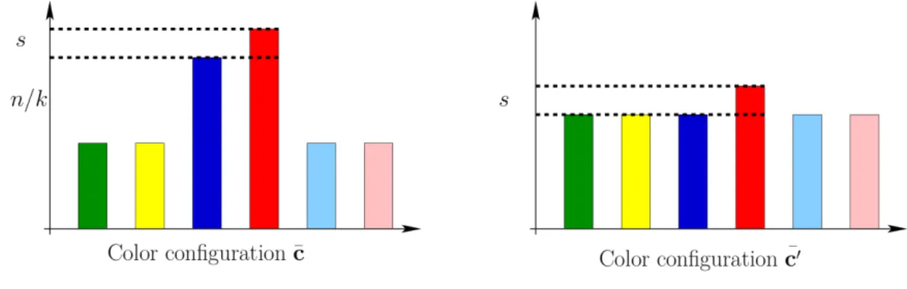
• (Almost validity / Almost plurality). The system is required to converge w.h.p. to an almost-agreement regime where all but a negligible bad set of nodes keep the same valid color. In the case of stabilizing Almost Plurality Consensus, the almost-validity property is replaced by the request to converge to an almost-agreement regime where all but a negligible bad set of nodes hold the color that was initially supported by the plurality of the nodes, assuming that there was some initial bias s w.r.t. all the other colors - see below for a definition of bias.

• (Stability). The convergence toward such a weaker form of agreement is only guaranteed to hold with high probability (in short, w.h.p.9) and only over a long period (i.e. for any arbitrarily-large polynomial number of rounds).

Note that the above definition does not require the property of termination. In particular, in dynamic distributed systems, nodes represent simple and anonymous computing units that are not necessarily able to detect any global property, let alone termination.

The crucial parameters in the analysis of (Plurality) Consensus processes are the number n of nodes, the number k of colors, and, in the case of Plurality Consensus, the initial bias towards the plurality color. The latter is characterized in terms of a parameter that only depends on the relative magnitude: Typically, this relative magnitude is defined in terms of the absolute difference or the ratio between c₁ and c₂. Moreover, several analyses of Consensus processes we describe in the following sections assume the presence of an F -bounded dynamic adversary that, in each round, can arbitrarily change the color of any subset of nodes of size at most F . In this framework, we say that a protocol is F -resilient if it guarantees the properties of Definition 2 even in the presence of F -bounded dynamic adversaries.

3

_{Voter dynamics}

The Voter Model, which for consistency we call here Voter dynamics, is arguably the simplest nontrivial dynamics: at each round, every node copies tha state of a neighbor sampled uniformly at random. Here, by nontrivial we mean that the node is updating its state in a meaningful way with respect to the states of its neighbors.

9 _{According to the standard definition, we say that a sequence of events En, n = 1, 2, . . . holds with high} probability if P (En) = 1 − O(1/nλ) for some positive constant λ > 0.

More formally, let G(V, E) be a connected graph with node set V (of cardinality n) and edge set E (of cardinality m). Let Σ be a palette of colors of size n. Let d(u) be the number of neighbours of u ∈ V .

Definition 3 (Voter dynamics). The Voter Model {Xt}t on G is the discrete time Markov

process where the state space is the set of color functions c : V 7→ Σ and its time evolution is determined by the following elementary dynamics (denoted as Voter dynamics):

• Each node initially supports a color in Σ;

• In each round one node is selected uniformly at random and it adopts the color of a neigh-bour sampled uniformly at random.

The asynchronous version of the Voter dynamics, in which at each round only one node chosen uniformly at random updates its state, has long been studied in statistical mechanics as a model for consensus formation in population of spinless individuals [KRBN10, Lig12, Ald13]. The study of the synchronous version of the model, in which all nodes update their state, has been first considered in Distributed Computing in [HP01] as a proportionate agreement protocol. The Proportionate Agreement problem is defined as follows. Given a network of n nodes, where each node is initially supporting a color out of a set of k possibilities, we require the system to eventually reach a configuration in which every node is supporting the same color and, moreover, the final color should equal i with a probability proportional to the volume10 _of

the initial set of nodes supporting i, for each i ∈ [k].

As usual, when the system reaches a configuration in which every node is supporting the same color, we say that the system has reached Consensus.

The Proportionate Agreement problem is a special case of Consensus, which the further constraint of a probability distribution on the color the system eventually agrees on.

As discussed in Section 1.1, many fundamental aspects of dynamics are often best described in the language of Markov chains. In the following sections, we present the fundamental results on the convergence probability and the convergence time of the Voter dynamics.

3.1 _{Fundamental results on the Voter dynamics}

It is immediate to see that absorbing states11_{of the Voter dynamics are the ones in which nodes} have reached consensus, i.e., those corresponding to monochromatic configurations. Probably the first and most natural question one may ask is with which probability each monochromatic configuration is reached, as a function of the initial color configuration.

[HP01] answered this question by providing, via an elegant martingale argument, the guaran-tee for employing the Voter dynamics as a protocol for the Proportionate Agreement problem, in which we want the system to reach consensus on color i with probability proportional to the volume of the set of nodes initially supporting color i.

10

The volume of a set of nodes S is defined as the sum of the degrees of nodes in S, in formulas vol(S) := P

u∈Sdu. In the general case of weighted graphs, we further have that duequals the sum of the weights of the edges incidents to u, namely du:=P

v∼uw(u, v).

11_{We remark that the term state is used in quite different ways in theory of Markov chains and in the distributed} computing literature: in distributed computing the term state usually refers to a single node and a full description of the system at a given time is referred to as configuration (thus, a configuration is often the vector of each node’s state); on the contrary, the term state in the theory of Markov chains corresponds to that of configuration in distributed computing. In this survey, for the sake of consistency, we employ the term state in the Markov-chain sense when referring to absorbing states.

Theorem 4 (Proportionate Agreement [HP01]). Let i be any color and e(0)_i be the volume of the nodes that support color i at t = 0; formally, e(0)_i = {P

u:c(0)_(u)=idu}. Then, e

(0) i

2m is the

probability that the Voter dynamics converges to the monochromatic configuration in which all nodes supports color i.

The next natural question that arises when considering a dynamics such as the Voter dynamics, is the speed with which consensus is reached. It turns out that also for the latter question, Voter dynamics is amenable to an elegant mathematical treatment: its convergence time can be analyzed via a duality with the coalescing random walks process [AF95].

Definition 5. The Coalescing Random Walks process (for short CRW) on G is a discrete time Markov process defined as follows:

• Each node initially holds one token.

• In each round, each node sends all its tokens to a neighbor chosen uniformly at random.

Figure 2: The diagram represent an instance of the CRW process, from left to right, in which an edge from u to v means that the token on u -if any- moves to v. In the diagram, after T = 4 rounds the number of random walks in the CWR process reduces to k = 2. The same diagram represents an instance of the Voter dynamics, from right to left, in which an edge from u to v means that u pulls v’s color. For the Voter dynamics as well, we see that the number of colors after T = 4 rounds is also 2. This is no coincidence, given that the two processes share the same random choices (i.e. black arrows).

The term coalescing in the name of the CRW process refers to the fact that, as soon as too tokens happen to be located on the same node, they will move together in the following rounds. Hence, we can imagine that they have “coalesced”.

It is easy to see that, by the process’ definition, all tokens in the CRW process are eventually located on a single node. The first occurrence of the latter event is thus referred to as the coalescing time. In fact, the following theorem draws a direct correspondence between the convergence time of the Voter dynamics and the coalescing time of the CRW process, allowing to study either of them by investigating the other (for a proof see e.g. Lemma 4 in [BCE+17]). An intuitive representation of the duality is also depicted in Figure 3.1.

Theorem 6 (Voter dynamics vs CWR). Let τ be the first round such that the Voter dynamics reaches consensus and let τ0 be the first round such that all the tokens of the CWR process are on the same node. A coupling between the Voter dynamics and the CWR process exists such that τ = τ0.

The coalescing time of the CRW process, and thus the corresponding consensus time for the Voter dynamics, can be studied on a variety of topologies by employing standard tools for the analysis of stochastic processes [HP01, KMTS19].

As an example, by combining Theorem 6 with the application of drift analysis techniques to the CWR process, we obtain the following theorem that provides the time after which at most k colors are still “alive” (for a proof, see e.g. Lemma 3 in [BCE+17]).

Theorem 7 (Color evolution on the complete graph). Let G be the complete graph, where each node has also a self-loop. Starting from an arbitrary initial configuration c on G, the Voter dynamics reaches a configuration c0 having at most k remaining colors w.h.p. in O(n_klog n) rounds.

More generally, by combining Theorem 6 with results on the meeting time of random walks on general graphs [TW93], we obtain the following general bound on the convergence time of the Voter dynamics.

Theorem 8 (Convergence time on general topologies). Let G be any connected undirected graph. Starting from an arbitrary initial configuration c on G, the Voter dynamics reaches consensus w.h.p. in O(n3log n) rounds.

4

_{Median dynamics}

If we consider an ordered color set hΣ,_{6i, then a simple consensus dynamics is the Min dynamics:} every node pulls a random neighbor (or a few of them) and then it recolors itself with the minimal color it sees.

Let us consider the synchronous PU LL model on a connected graph G(V, E) and assume that the dynamics starts with any color configuration with one node u having the minimal value min.12 _{Then it is not hard to see that the resulting process is equivalent to the popular}

single-source broadcast on the PU LL model which has been widely studied in algorithm theory [CLP11, CCD+16, Gia16]: For instance if the graph is regular and it has high conductance13, the Min dynamics turns out to be fast, i.e. O(log n) [CLP10].

However, this dynamics is not reliable in network scenarios where the state of some, few nodes can be corrupted by an adversary. Indeed, to just get a simple intution about this breakable behaviour, let us consider the time the system has reached the monochromatic configuration in which all nodes support the initial minimal value. Then it suffices that the adversary corrupts the state of just one node by setting its value to a smaller value than min and this small change immediatly causes the system to start a new process where all nodes will change the state again. If the adversary makes this small change frequently, it is clear that the system will never stays over an (almost-)stable regime.

In [DGM+11], Doerr et al proposed another natural dynamics on the synchronous PU LL model that works on any ordered color set: the Median dynamics. Its local updating rule is

12

Notice that if the minimal value is initially supported by more nodes, then, clearly, the process will be stochastically not slower than the the single-source process.

13

Informally speaking, the conductance of a connected graph is a fundamental parameter φ ∈ (0, 1] which is large for highly-connected graphs (such as the complete graphs), while it is small when the graph contains some bottleneck.

very simple: at every round, every node u pulls the colors x(v) and x(w) of 2 neighbors chosen independently and uniformly at random; then, the color of node u at the next round will be the median among x(u), x(v), and x(w). Notice that, differently from getting the average of the values, the median rule does not introduce new values, i.e. values that were not supported by any node in the previous round.

Doerr et al provide an analysis of the Median dynamics on the complete graph for both the fault-free model and in presence of an F -bounded adversary that can corrupt the state of at most F nodes at every round.

The first result essentially shows that, if no node of the complete graph is ever corrupted, then the Median dynamics let the median value to spread fast over the network, as the minimal one in the Min dynamics.

Theorem 9 (Median rule in the fault-free case [DGM+11]). Starting from any color configura-tion of the complete graph, w.h.p., the Median dynamics guarantees the following properties:

• (Convergence time.) It takes O(log n) rounds to converge to a stable monochromatic con-figuration.

• (Median computation.) The system converges to the configuration where all nodes support the median value.

As remarked above, however, the main interest on this dynamics, lies in its tolerance w.r.t. node corruptions.

Doerr et al show that the Median dynamics is in fact a natural and efficient almost-stabilizing consensus protocol against O(√n)-bounded adversary on the complete graph (see Definition 2). More precisely, they prove the following results.

Theorem 10 (Median rule vs Byzantine nodes [DGM+_{11]). Let the Median dynamics start}

from any color configuration of the complete graph. Assume there is an F -bounded adversary with F = O(√n). Then, the following properties hold:

• (Almost stability.) The system converges to an almost-stable regime where all but at most O(F ) nodes agree on some legal color j ∈ Σ and this regime lasts for any poly(n) many rounds, w.h.p.

• (Convergence time.) The time to reach this almost-stable regime is bounded by O(log |Σ| · log log n + log n), w.h.p.

• (Median computation.) The legal value j “computed” by the system in the almost-stable regime is between the (n/2−c√n log n)-largest value and the (n/2+c√n log n)-largest value of the initial values, w.h.p, for a suitable constant c > 0.

Key-ingredients of the analysis. The analysis of the Median dynamics proposed in [DGM+11] considers two main cases.

They first consider the binary case, i.e., Σ = {0, 1}. Notice that, in this setting, the update rule of the Median dynamics turns out to be equivalent to the majority rule: every node takes the most frequent value he sees among its own value and the values of the two randomly-selected neighbors (notice that there cannot be ties). In this case, the analysis works in 3 phases depending on the magnitude of the bias s = |c₀− c₁| of the starting configuration (recall that c_i is the number of nodes supporting color i).

(Case 1.) If s _{> n/4, then the size of the minimal color is proved to decrease at a} double-exponential rate, w.h.p.: this implies that after O(log log n) rounds the minimal color will dis-appear, w.h.p.

(Case 2.) If the bias s is such that Ω(√_{n log n) 6 s 6 n/4, then the analysis focuses on the} evolution of the random variable s over a logarithmic time-window. Indeed, it is proved that, at every round, the bias increases by a constant factor, w.h.p. and, thus, after O(log n) rounds, the system falls into the range of Case 1. In both Cases 1 and 2, the analysis essentially relies on a strong expected drift towards the majority color and some standard concentration arguments (i.e. Chernoff’s bounds).

(Case 3.) If the system starts from some configuration having bias s <√n log n then the analysis requires different arguments since the drift of the bias is too weak for applying any step-by-step concentration argument. When s₆√n, they essentially prove that, thanks to the variance of the process, at the next round there is constant probability that the bias reaches a magnitude of γ√_{n for some suitable constant γ > 0. Once the system reaches a bias s > γ}√n, then s is likely to increase at the next round. However, differently from the previous two cases, this event cannot be guaranteed to hold w.h.p. at every round and an amortized, more complex argument is required. To this aim, the authors make use of a useful bound on the hitting time on a Markov chain Zt (t = 1, 2, . . .) defined on a finite set of integers {0, 1, . . . , q} which have some

drift properties towards increasing values (see Claim 2.9 in [DGM+11] for a formal statement of the bound). Setting Z_t:= bs/(γ√n)c and q = b(n/2)/γ√nc, the bound on the hitting time implies that after O(log n) rounds, the Markov chain hits a state j such that j _{> α log q, for} some suitable constant α > 0. We thus have that the bias reached by the system after O(log n) rounds turns out to be Ω(√n log n), w.h.p. which let the analysis go back to Case 2 above.

The analysis of the multivalued case (i.e. |Σ| _{> 3) relies on some arguments which} signif-icantly depart from the binary case. It is important to observe that in the multivalued case, the Median dynamics has a local rule which is different from the majority one and it is not symmetric w.r.t. to the color values. Indeed, by definition, the median value plays a preferential role among the colors. Informally speaking, the analysis introduces a sort of rank of the colors: the more the color is close to the median, the more this rank is high and it is maximum for the median value. Then, it is shown that the dynamic makes colors with highest rank to increase their own supporters at every round. This process is then proved to converge within O(log n) time to a configuration with at most only two “median” colors and, thus, the analysis can go back to the binary case. The presence of the adversary further complicates the process analysis and it requires the additive factor log |Σ| · log log n in the obtained convergence time claimed in Theorem 10.

On the validity property. It is important to investigate the kind of agreement which is guaranteed by Theorem 10 for the Median dynamics. The property of validity which is required in the standard definition of Consensus against Byzantine nodes (i.e. the Byzantine Agreement) is that the system must converge to an almost-stable configuration where all but a small fraction of node support a valid color, i.e., a color which was supported by at least one non-corrupted node in the initial configuration. Unfortunately, the analysis in [DGM+11] leading to Theorem 10 does not guarantee this validity property: in particular, it is an interesting open issue to establish a bound on the fault tolerance parameter F for which the Median dynamics guarantees this stronger, classic validity property. We believe the real bound needs to be small, much smaller than F = O(√n). To motivate our intuition here, we invite the reader to think about the starting configuration with n/2 nodes colored with value 0 and n/2 nodes colored with value 2. Then, the adversary takes m = Θ(polylog (n)) nodes at every round and it colors them with value 1. Non-rigorous, “mean-field” arguments lead us to guess that, with non-negligible probability, the non-valid, “median” value 1 will spread faster than any possible growth of the

other two valid colors, thus forcing the system to converge to the non valid color 1.

The Median dynamics over non-complete topologies. We are not aware of rigorous analysis of the Median dynamics that works over non-complete graphs. However, in the binary case, the Median dynamics turns out to be equivalent to the popular majority dynamics known as 2-Choices (see Section 5.1) and the latter has been recently analyzed over regular expander graphs.

5

Majority dynamics

The Median dynamics protocol fully relies on the presence of some total ordering on the color set Σ. In some scenario, such as the ones inspired by biological systems, this assumption might be not reasonable: Particles and bio-inspired agents may have no ordering on the possible states they can assume. Moreover, as remarked in the previous section, it is unknown (and, in our opinion, unlike) whether Median dynamics can guarantee the important validity property, with high probability.

A class of natural dynamics, requiring no color ordering, are those based on majority rules. In the synchronous PU LL model, h-Majority dynamics works as follows:

Definition 11 (h-Majority dynamics). At every round, every node u samples h > 1 neighbors, independently and uniformly at random.

Then, u gets the plurality color among those in the sample; if there is no plurality in the sample, u gets the first sampled color.14

An important instance of the h-Majority dynamics is the 3-Majority dynamics. The reason of its relevance is essentially that a sample of size 3 is the minimal one to hope for a different behaviour from the Voter dynamics seen in Section 3. Indeed, looking at only two random nodes and breaking ties uniformly at random would yield a coloring process equivalent to the Voter dynamics, and the latter it is known to converge to a minority color with constant probability even in the case of 2-color initial configurations having a large initial bias (see Section 3).

Another popular majority rule is the 2-Choices. It differs from the 3-Majority dynamics on the fact that node u samples the colors of (only) two random neighbors. Then, it applies the plurality rule (like 3-Majority dynamics) among such two random colors and its own color. So, in the 2-Choices, the updating rule deterministically depends on the current state of the node while 3-Majority dynamics gives no special role to the current state of the node. As we will see later in Subsection 5.3, even though the expected behaviours of 3-Majority dynamics and 2-Choices are equivalent, their “real” behaviours turn out to be significantly different when the number k of the initial colors is large.

5.1 _{2-Choices dynamics}

It is easy to see that, in the binary case (i.e. |Σ| = 2), Median dynamics turns out to be equivalent to 2-Choices. As for the latter, we thus have the following immediate consequences of the results [DGM+11] shown in the previous section.

Corollary 12 (Two colors, [DGM+_{11]). Let Σ = {0, 1}. Let the system start from any color}

configuration and assume there is an F -bounded adversary with F = O(√_{n). Then, 2-Choices} is a stabilizing almost (Plurality) Consensus protocol. In more detail, it guarantees the following properties:

14

• (Almost Stability.) The system converges to an almost-stable regime where all but at most O(F ) nodes agree on some valid color j ∈ Σ and this regime lasts for any poly(n) many rounds, w.h.p.

• (Convergence Time.) The time to reach this almost-stable regime is bounded by O(log n), w.h.p.

• (Plurality Consensus.) Assume the initial configuration has bias s towards a plurality color such that s_{> c}√n log n, for some constant c > 0. Then, the color the system converges to in the almost-stable regime is the plurality one, w.h.p.

As we will also see in further results described in this survey about dynamics for Plurality Consensus, the bias threshold √n log n will show up rather often. Informally speaking, this is due to the fact that the standard deviation (in the binary case) of the studied process is order of √

n. This implies that if the system starts from bias “too” close to the magnitude of the standard deviation, some anti-concentration bounds say us that the system can change plurality color in one round, with non-negligible probability. Thus, in order to preserve the initial plurality and to get results in concentration, the system must start from a bias Ω(√n log n).

The multi-color case. A deep analysis of this dynamics for k = O (nε) has been recently presented by Elsässer et Al in [EFK+17]. They consider initial configurations c = (c1, c2, . . . , ck)

having some initial bias s = c1− c2 and show that this dynamics is an efficient, fault-tolerant

protocol for Plurality Consensus.

Theorem 13 (More colors, biased initial configurations, [EFK+17]). Let Σ = {1, 2, . . . , k} with k = O (nε) where ε is a sufficiently small constant15_{. Then 2-Choices is a stabilizing}

almost Plurality Consensus protocol. In detail, let the system start from any color configuration c = (c1, c2, . . . , ck) with bias s > γ

√

n log n where γ > 0 is some positive constant and assume there is an F -bounded adversary with F _{6 c1}(c1− c2)/(8n). Then,

• (Almost Stability.) The system converges to an almost-stable regime where all but at most o(n) nodes agree on some valid color j ∈ Σ and this regime lasts for any poly(n) many rounds, w.h.p.

• (Convergence Time.) The time to reach this almost-stable regime is bounded by O((n/c1) log n),

w.h.p. Notice that, since it always holds that c_{1 > n/k, then the latter bound also implies} the bound O(k log n).

• (Plurality Consensus.) The color the system converges to in the almost-stable regime is the plurality one, w.h.p.

Moreover, if the initial configuration c is such that s_{> γ}√n log n and cj = c2 for j = 3, . . . , k,

then the expected time required to converge to the almost-stable regime is Ω(n/c₁+ log n). The proof of the above theorem relies on the following arguments. By using Chernoff bounds, Elsässer et al. show that the number of nodes which change their color to 1 is larger than the number of nodes which switch to color 2. From the lower bound on the initial bias s assumed by the above theorem, the bias increases by some positive factor in the next round w.h.p, and using a union bound over an O((n/c₁) log n) sequence of rounds, they get the claimed upper bound on the convergence time. The main technical issue lies in bounding the number of nodes moving to color 1 and 2. Indeed, just applying a Chernoff bound to every single color community would

15

lead to much weaker results. Instead, they carefully aggregate colors when considering the nodes moving to one color to the other. Intuitively, the difficulty lies in the sheer number of initial colors the new analysis allows. Their total support may significantly exceed c1.

Starting from unbiased configurations. A natural issue on 2-Choices concerns its be-haviour when starting from balanced configurations, i.e., whenever s turns out to be relatively small, say s = o(√n).

This setting has been analyzed in a recent work by Ghaffari et Al in [GL18]. They provide a tight bound on the convergence time starting from any configuration with a polynomially-bounded number of colors, i.e., k = O(pn/ log n).

Theorem 14 (More colors, balanced intial configurations [GL18]). Let Σ = {1, 2, . . . , k} with some k = O(pn/ log n). Then, 2-Choices is a stabilizing almost Consensus protocol. In more detail, let the system start from any color configuration c and assume there is an F -bounded adversary with F = O(√n/k1.5). Then,

• (Almost stability.) The system converges to an almost-stable regime where all but at most o(n) nodes agree on some valid color j ∈ Σ and this regime lasts for any poly(n) many rounds, w.h.p.

• (Convergence time.) The time to reach this almost-stable regime is bounded by Θ(k log n), w.h.p.

The analysis in [GL18] uses and improves an approach which has been previously introduced by Becchetti et Al in [BCN+_{16] to analyze 3-Majority dynamics in a similar setting (see} Subsection 5.2). When the process starts from an (almost-)balanced configuration, any first-moment analysis of the expected values of the color size is almost useless: in average, the system stays in the same (almost-)balanced configuration. On the other hand, the real process starts to jump randomly over several (almost-)balanced configurations thanks to its variance until the symmetry among the color sizes is broken: we can then observe the birth of some plurality color that starts to increase rapidly. It thus follows that a non-standard second-moment analysis is required that makes use of anti-concentration bounds for multinomial distributions.

Analysis over non-complete topologies. In [CER14], Cooper et al. analyze, for the first time, the random process yielded by applying 2-Choices over d-regular graphs. They consider the binary case and give different bounds on the convergence time depending on several input parameters, such as node degree d, initial bias s, and on which class of regular graphs the process runs on. We give here two of the bounds mentioned above.

The first result concerns a graph which is sampled uniformly at random from the class of d-regular graphs of n nodes.

Theorem 15 (Binary case on sparse random graphs [CER14]). Let G be a d-regular random graph with d ₆√_{n and assume the initial color configuration has bias s > γn/}√d, for a large enough constant γ > 0. Then, with probability 1 − o(1), 2-Choices converges to the initial majority within O(log n) rounds.

The second results provided in [CER14] concerns (deterministic) regular graphs having good expansion properties. A graph G is said to be an (edge) ε-expander if, for any node subset S of size not larger than n/2, it holds e(S, V − S)_{> ε|S|, where e(S, V − S) denotes the number of} edges in the cut E, V − S). The expansion properties of the underlying d-regular graph G(V, E) can be expressed in terms of the spectral gap λ₁−λ₂, where λ₁and λ₂are respectively the largest and the second-largest (in absolute value) eigenvalue of the transition matrix P = (1/d) · A of G (A denotes the symmetric adjacency matrix og G - see also Section 7.2 for further useful concepts

in spectral graph theory). If G is connected and not bipartite then it holds that λ₁ = 1, λ2< 1

and |λ_{i| > 1, for every i = 1, . . . , n. Roughly speaking, the larger is the spectral gap the larger is} the (edge) expansion of the graph. This fact is formalized by the well-known Expander Mixing lemma which is a key-ingredient in Cooper et al.’s analysis:

Lemma 16 (Expander mixing lemma [AC88]). Let G be a connected, non-bipartite d-regular graph, then, for any S, T ⊂ V , it holds

    e(S, T ) −d|S| · |T | n     6 λ2 dp|S| · |T | .

Theorem 17 (Binary case on expander graphs [CER14]). Let G be a d-regular graph with d 6 √n and second largest eigenvalue 0 < λ2 < 1, and assume the initial color configuration

has bias s_{> γλ2}n, for a large enough absolute constant γ > 0. Then, with probability 1 − o(1), 2-Choices converges to the initial majority within O(log n) rounds.

We first notice that the success probability guaranteed in the above theorems is weaker than that defined in the standard notion “w.h.p.” we adopt in this paper.

Roughly, the proofs of the above two bounds on the convergence time of the 2-Choices process rely on the following key-ingredients. Let us look at the color configuration of G at a generic round t_{> 0 and consider the sizes c}1 and c2 of subsets C1 and C2 of nodes that support

the majority color and the minority one, respectively. Let us also define the two random variables ∆12and ∆21 which count the number of 1-colored (2-colored) nodes that will get color 2 (1), at

round t + 1. A first simple but crucial fact is that, if a 2-colored node changes its color at the next round, then, according to the 2-Choices, it must have sampled the other color twice from its neighborhood, i.e., from some neighbors that must belong to C₁. Then, it is easy to verify that that the expected number E [∆21] of nodes that makes this change is an increasing function

of the expansion of subset C2, i.e., of the size e(C2, V − C2 = C1). A symmetric argument clearly

holds for E [∆₁₂]. Now, if G is a good expander, say λ2< 1/3, their analysis shows that Lemma

16 implies a positive drift for the expectation E [∆12− ∆21]. This analysis is organized in few

consecutive phases that depend on the range the random variable c1 (and, thus, c2) currently

lies on during the process. Several technical issues are neglected by our informal description above which are essentially due to get concentration bounds even when the considered random variables takes small values.

Further analysis of the 2-Choices dynamics on non-complete graphs consider the binary case over non-regular expander graphs [CER+15] and the multi-color case on regular expander graphs [CRRS17]. The techniques introduced in these works are combined in [CNS19] with the community-sensitive labeling scheme introduced in [BCN+17c] (see Section 7 for further details on the latter), in order to use the 2-Choices dynamics to perform community detection.

Finally, the 2-Choices has also been proposed in recent work by Cruciani et al. [CNNS18] as a natural, simplistic model of competition among opinions in social networks having core-periphery topologies. The author consider a network model where a densely-connected subset of agents, the core, holds a different opinion from the rest of the network, the periphery. Then, depending on the strength of the cut between the core and the periphery, they provide analytical evidence of the existence of a phase-transition phenomenon: Either the core’s opinion rapidly spreads among the rest of the network, or a metastability phase takes place, in which both opinions coexist in the network for superpolynomial time. This result sheds light on the influence of the core on the rest of the network, as a function of the core’s expansion over the latter. Moreover, this represents the first analytical result which shows a heterogeneous behavior of a “pure” majority dynamics as a function of structural parameters of the network; similar behaviour have been previously proved for averaging dynamics only, that is, when opinions admit numerical operations (see Section 5).

5.2 _{The 3-Majority dynamics}

From an historical point of view, the study of the 3-Majority dynamics started on the ground of the results obtained for the Median dynamics by Doerr et Al in [DGM+11] that we have described in Section 4. Indeed, as discussed in that section, the Median dynamics is a fault-tolerant, efficient dynamics which, however, does not guarantee to reach a valid consensus (see the discussion at the end of Section 4). This fact naturally leads researchers to look for efficient dynamics having this further fundamental property.

3-Majority dynamics for Plurality Consensus

The 3-Majority dynamics was the first dynamics which has been proved to be a fault-tolerant protocol for (valid) Plurality Consensus. Such results were proved by Becchetti et Al in [BCN+17a].

Theorem 18 (Plurality Consensus [BCN+17a]). Let Σ = {1, 2, . . . , k} with any with k _{6 n.} Then, 3-Majority dynamics is a stabilizing almost Plurality Consensus protocol. In details, let λ be any value such that λ < √3_{n, and let c be any initial color configuration, with c}

1 > n/λ

and s _{> 72}√2λ n log n. Assume there is an F -bounded adversary with F = o(s/k). Then, the 3-Majority dynamics guarantees the following properties:

• (Almost-stable Plurality Consensus.) The system converges to an almost-stable regime where all but at most o(n) nodes agree on the ( valid) initial plurality color and this regime lasts for any poly(n) many rounds, w.h.p.

• (Convergence time.) The system converges to the plurality color within O (λ log n) time, w.h.p.

The analysis achieving the theorem above is accurate enough to get an interesting form of the upper bound that does not depend on k. Indeed, when the initial plurality size c₁ is larger than n/λ(n) for any function λ(n) such that 1 _{6 λ(n) <} √3_{n and s > 72}p2λ(n) n log n, the

process converges within time O (λ(n) log n), w.h.p., no matter how large k is. Hence, when c1 > n/polylog (n) and s >pn polylog (n), the convergence time is polylogaritmic.

Becchetti et Al [BCN+17a] show that the upper bound on the convergence time in Theorem 18 is tight for a wide range of the input parameters. When k _{6 (n/ log n)}1/4, they in fact prove a lower bound Ω(k log n) on the convergence time when the 3-Majority dynamics starts from some configurations with bias s _{6 (n/k)}1−ε, for an arbitrarily small constant ε > 0. Observe that this range largely includes the initial bias required by the upper bound whenever k 6 (n/ log n)1/4. So, the linear-in-k dependence of the convergence time cannot be removed for a wide range of the parameter k.

The analysis also provides a clear picture of the process yielded by the 3-Majority dynam-ics. Informally speaking, the larger the initial value of c1 is (w.r.t. n), the smaller the required

initial bias s and the faster the convergence time are. On the other hand, the lower-bound argument shows, as a by-product, that, from balanced configurations, the initial plurality size c1 needs Ω(k log n) rounds just to increase from n/k + o(n/k) to 2 n/k.

Another natural issue is to analyze the process under weaker assumptions on the initial bias. Becchetti et Al [BCN+17a] show that there are initial configurations with bias s = O(√kn) for which the bias decreases in a single round with constant probability. This implies that the assumption on the magnitude of the initial bias is in a sense (almost) tight if one wants to prove a monotonic increase of the bias in every round with high probability, as they did in proving the upper bound on the convergence time.

Analysis over non-complete topologies. Very recently [KR19], the 3-Majority dynamics was analyzed over a class of dense graphs with minimum degree d = Ω(nα_{), where Ω((log log n)}−1_{) 6}

α 6 1, and starting from random, biased binary configurations . In more detail, [KR19] prove that if initially each vertex chooses red with probability greater than 1/2 + δ, and blue other-wise, where δ _{> (log d)}−β, for some β > 0, then the dynamic solves Plurality Consensus within O(log log n + log(δ−1)) rounds, w.h.p.

3-Majority dynamics for Consensus

In [BCN+_{16], Becchetti et al extend the analysis of 3-Majority dynamics in the multi-color} case from any (even balanced) initial configuration in the presence of an adaptive F -dynamic adversary and of the F -static adversary (in the latter, the adversary looks at the initial configu-ration, then changes the opinion of up to F nodes and, after that, no further adversary’s actions are allowed).

Theorem 19 (Consensus [BCN+16]). Let k_{6 n}α for some constant α < 1 and F = β√n/(k52 log n)

for some constant β > 0. Starting from any initial configuration having k valid opinions, 3-Majority dynamics reaches a stabilizing almost-consensus in the presence of any F -dynamic adversary within O((k2√log n + k log n)(k + log n)) rounds, w.h.p.

Moreover, the same bound on the convergence time holds in the presence of any F -static adver-sary with a larger bound on F , i.e., F = n/k −√kn log n.

Not assuming a large initial bias of the plurality opinion considerably complicates the anal-ysis. Indeed, the major open issue here is the analysis from (almost) uniform configurations, where the system needs to break the initial symmetry in the absence of significant drifts towards any of the initial opinions. Notice that the phase before symmetry breaking is the one in which the adversary has more chances to cause undesired behaviours: Long delays and/or convergence towards non-valid opinions. Let us consider the non-adversarial case. When the configuration is (approximately) uniform, the process exhibits no significant drift toward any fixed opinion. Interestingly, things change if we consider the random variable c(t)_m, indicating the smallest opin-ion support at round t. Let j _{6 k be the number of active opinions in a given round t, it is first} proved that the expected value of c(t)_m always exhibits a non-negligible negative drift:

Ehc(t+1)_m | c(t) _{= ˆc}i_{6 c} m− ε

√ n

j3/2, for some constant ε > 0 . (1)

The analysis then proceeds along consecutive phases, each consisting of a suitable number of consecutive rounds. If the number of active opinions at the beginning of the generic phase is j, it is shown that, with positive constant probability, c(t)_m vanishes within the end of the phase, so that the next phase begins with (at most) j − 1 active opinions.

Clearly a good bound is needed on the length of a phase beginning with at most j opinions. To this aim, the authors derive a new upper bound on the hitting time of stochastic processes with expected drift that are defined by finite-state Markov chains [LPW09]. Thanks to this result, they can use the negative drift in (1) to prove that, from any configuration with j _{6 k} active opinions, c(t)_m drops below the threshold n/j −√jn log n within O(poly(j, log n)) rounds, with constant positive probability: This “hitting” event represents the exit condition from the symmetry-breaking stage of the phase. Indeed, once it occurs, we can consider any fixed active opinion i having support size c_i below the above threshold (thanks to the previous stage, we know that there is a good chance this opinion exists): It is then shown that ci has a negative

drift of order Ω(ci/j). This allows to prove that ci drops from n/j −

√

O(poly(j, log n)) further rounds, with positive constant probability. This interval of rounds is the dropping stage of the phase.

Ideally, the process proceeds along k consecutive phases, indexed as j = k, k − 1, . . . , 2, such that we are left with at most j − 1 active opinions at the end of Phase j. In practice, there is only a constant probability that at least one opinion disappears during Phase j. However, using standard probabilistic arguments, it is proved that, w.h.p., for every j, the transition from j to j − 1 active opinions takes a constant (amortized) number of phases, each requiring O(poly(j, log n)) rounds.

The upper bound in Theorem 19 was later improved in [GL18], using a more refined analysis that does not require k consecutive phases (see Theorem 14 and the discussion below it).

5.3 _{2-Choices vs 3-Majority dynamics}

The results described in the previous two subsections naturally lead to investigating the main differences between the 2-Choices and the 3-Majority dynamics. This issue has been recently addressed by Berenbrink et Al in [BCE+17].

We notice that Theorem 14 provides an upper bound on the convergence time for the 2-Choices for a limited number of colors (i.e. k = O(pn/ log n)). On the other hand, when k is almost linear in n, the behaviour of the 2-Choices turns out to be rather “lazy”, as stated by the following result.

Theorem 20 (2-Choices: Many colors, balanced initial configurations [BCE+_{17]). Let Σ =}

{1, 2, . . . , k} with some k = Ω(n/ log n). Let the system start from any color configuration c = (c1, c2, . . . , ck) such that c1 = O(log n), then, the 2-Choices needs Ω(n/ log n) rounds to

converge to a monochromatic configuration, w.h.p.

The proof of the above theorem shows that, when started from an almost balanced config-uration, the convergence time is dominated by the time it takes for one of the colors to gain a community of supporters of size ω(log n). The analysis adopts the following line of reasoning. If the system lies in an almost-balanced configuration with an almost linear number of colors, then most nodes are likely to see two different colors in their respective 2 randomly-selected neighbors. This implies that, according to the 2-Choices updating rule, such nodes will keep their own color for several rounds. In other words, under this setting, the variance of the process is relatively low.

Does the 3-Majority dynamics show the same “lazy” behaviour when it starts from many-colors, unbiased configurations? The answer to the above question is given by the following result.

Theorem 21 (3-Majority dynamics: Many colors, balanced initial configurations [BCE+17]). Let Σ = {1, 2, . . . , k} with any k_{6 n. Starting from an arbitrary configuration, the 3-Majority} dynamics converges to a monochromatic configuration within O(n3/4log7/8n) rounds, w.h.p.

Theorems 20 and 21 together show that there can be a polynomial gap between the conver-gence time of 2-Choices and 3-Majority dynamics: one should note that this gap is in stark contrast not only to the expected behavior of both processes (which is identical - see for instance [BCN+17a, BCE+17]) but also to the setting when k = O(nε) (for some ε < 1) and a good bias towards one color: essentially, we have seen in the previous subsections that, in that case, both processes exhibit the same asymptotic runtime O(k · log n).

Interestingly enough, the proof of Theorem 21 introduces (and exploits) a new coupling between the 3-Majority dynamics and the Voter dynamics (see Section 3). Berenbrink et al. show that the time needed by 3-Majority dynamics to reduce the number of colors to