Publisher’s version / Version de l'éditeur:
32nd AIAA Aerodynamic Measurement Technology and Ground Testing
Conference, 13-17 June 2016, Washington, D.C., 2016-06
READ THESE TERMS AND CONDITIONS CAREFULLY BEFORE USING THIS WEBSITE. https://nrc-publications.canada.ca/eng/copyright
Vous avez des questions? Nous pouvons vous aider. Pour communiquer directement avec un auteur, consultez la
première page de la revue dans laquelle son article a été publié afin de trouver ses coordonnées. Si vous n’arrivez pas à les repérer, communiquez avec nous à [email protected].
Questions? Contact the NRC Publications Archive team at
[email protected]. If you wish to email the authors directly, please see the first page of the publication for their contact information.
NRC Publications Archive
Archives des publications du CNRC
This publication could be one of several versions: author’s original, accepted manuscript or the publisher’s version. / La version de cette publication peut être l’une des suivantes : la version prépublication de l’auteur, la version acceptée du manuscrit ou la version de l’éditeur.
For the publisher’s version, please access the DOI link below./ Pour consulter la version de l’éditeur, utilisez le lien DOI ci-dessous.
https://doi.org/10.2514/6.2016-4161
Access and use of this website and the material on it are subject to the Terms and Conditions set forth at
Pressure-sensitive paint measurements on a moving store in the NRC
1.5 m blowdown wind tunnel
Mébarki, Youssef
https://publications-cnrc.canada.ca/fra/droits
L’accès à ce site Web et l’utilisation de son contenu sont assujettis aux conditions présentées dans le site LISEZ CES CONDITIONS ATTENTIVEMENT AVANT D’UTILISER CE SITE WEB.
NRC Publications Record / Notice d'Archives des publications de CNRC:
https://nrc-publications.canada.ca/eng/view/object/?id=eb2ee871-835c-4c21-82d5-36c44ba3a252 https://publications-cnrc.canada.ca/fra/voir/objet/?id=eb2ee871-835c-4c21-82d5-36c44ba3a252
Pressure-Sensitive Paint Measurements on a Moving Store in
the NRC 1.5 m Blowdown Wind Tunnel
Youssef Mébarki and Ali Benmeddour
National Research Council, Ottawa, Ontario, K1A0R6, Canada
The pressure-sensitive paint technique (PSP) is used to measure the model surface pressures in wind tunnel testing. In the NRC 1.5 m blowdown wind tunnel, the testing time is limited between 10 to 100 sec, depending on the mass flow rate and the tunnel geometry (2D or 3D test section). Traditionally, production PSP testing required a stationary model during the image acquisition. In order to optimize the testing time, a novel approach for PSP testing in production wind tunnels has been implemented to acquire PSP data on continuously moving objects. This type of testing (pitch and roll sweeps) is the usual method of testing in the 1.5 m blowdown wind tunnel, when conventional instrumentation is used (balance forces and pressure tap data). The measurement method is based on the single shot lifetime method, using UV-LED excitation pulses and 49 Hz image acquisition with a scientific CMOS (sCMOS) camera. The method was demonstrated on the fins of a generic store, tested at M = 0.6, 0.8 and 1.0, at angles of attack from -10° to 20°, and moving at variable pitch rates of 3°/s, -6°/s and 9°/s. The PSP data on the moving model (pitch sweep mode) was compared to PSP data on steady model (pitch step mode), to determine the maximum acceptable pitch rate. The store model was not instrumented with pressure taps and the PSP data from the pitch sweep test was compared with computational fluid dynamics (CFD) simulations. A single Cp offset from the CFD simulations was used to compensate for the model global temperature changes.
Nomenclature
A,a = Coefficients of pressure and temperature sensitivity (e.g. slopes)
B, b = Coefficients of pressure and temperature sensitivity (intercept)
Cp = Pressure coefficient
t = Delays
f = Fraction of the excitation pulse measured in the second image
I = Intensity
M = Mach number
P = Static pressure
P0 = Total pressure
R = Intensity ratio between first and second image
SNR = Signal to noise ratio
T = Temperature
t = Time
t0 = External trigger period
= PSP luminescence lifetime Subscript
ref = Reference (wind-off) L = Light
I = Camera interframing
1, 2 = Relative to first and second images
I.
Introduction
he typical mode of operation of the NRC 1.5 m wind tunnel is the continuous pitch sweep mode, where the
Unlike continuous wind tunnels, the NRC 1.5 m wind tunnel is a pressurized blowdown facility that can operate during 10 sec to 100 sec depending on the flow conditions. For instance, at M = 1, P0 = 21 psi, the useful run time, before running out of air, is about 25 sec.
Traditionally, the PSP data acquisition in the facilities of the Aerodynamics Laboratory has been performed on stationary models, in a pitch step mode. In this mode, the model is positioned at the incidence of interest and the PSP images are collected. The model is then moved to the next angle, and data collection resumed.
There are several advantages to the pitch step operation for PSP. First, it offers the ability to increase the signal to noise ratio (SNR), using long exposure times or time-averaging over a large number of images. Also, since the model is at rest, the paint response time to pressure changes has no effect on the data accuracy. Figure 1 displays an illustration of a pitch step run with 5 data points, at 5° pitch angle increments. The total number of images per step can vary by an order of magnitude depending on the frame rates of the cameras selected for the test.
Figure 1: Example of a pitch step run with 5 steps, 4 sec per step.
The advantage of the pitch sweep mode of operation is that it permits the collection of more data points in a single run. It is then possible to combine in a single run, angle sweeps (pitch, roll and the combination of the two) and Mach number and/or total pressure changes, thus making optimal use of the limited run time.
The PSP acquisition can also be performed on a continuously moving model, if the exposure time can be reduced to less than a few milliseconds. The lifetime method seemed ideal for this type of application: it uses short excitation pulses (<100s), and the duration of the luminescence does not exceed 200s in most applications.
The traditional lifetime method using on-chip accumulation, requires multiple (~10000) pulses to accumulate enough photons on the sensor,1 and is not compatible with a moving model. The present study demonstrates a PSP application on a moving model.
The originality of the present work is the use of UV LED sources and low-noise scientific CMOS cameras operated at 49 Hz to perform single shot lifetime method on a moving object.2 Also, a simplified data processing pipeline on a model not equipped with pressure taps is proposed and demonstrated, using CFD simulations as the baseline data.
II.
Test Description
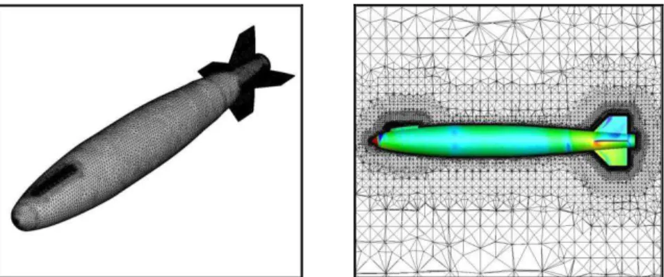
The model is a 40%-scale model of a GBU-38 store mounted on a straight sting and equipped with nose strakes (see Figure 2). The fins have of a maximum thickness of 2.3 mm near the center body, and slanted leading edges and sides. No pressure taps were available to assess the accuracy of the PSP data on the fins. The store center body was not painted with PSP to eliminate self-illumination between the normal surfaces. The model length was less than 1 m, and the maximum distance between two opposite fin edges was about 200 mm. In the following, the origin of the axis system is the store nose, with x being the longitudinal direction and z being the vertical direction.
As shown in Figure 2, only the upper surfaces of the store horizontal fins were painted with PSP. Six markers were placed on the top surfaces of the fins to allow image processing. The markers were 0.1 mm thick retroreflective circular tapes. The markers physical coordinates were determined by model scanning (Creaform HandyScan 3D). The paint was applied directly on the model fins made of steel. The paint thickness was measured with a thickness gauge (Positector 6000) to be on average 7+/-1m.
Figure 2: Left: GBU-38 store with nose strakes. Right: Store horizontal fins painted with PSP.
The PSP camera and 3 LED lamps (described in the next section) were mounted in the plenum of the test section, viewing the model through 3” diameter ceiling windows.
The camera selected for this acquisition is the Zyla 5.5 camera from Andor, equipped with a 5.5 Mpixel scientific CMOS sensor. This camera was selected because of its high resolution and frame rates, low read-out noise and short inter-framing times.3 It has USB3 connectivity delivering a maximum of 53 Hz images with 16-bit dynamic range. In order to increase the amount of light collected by the camera, 3x3 pixel binning was used, reducing the resolution of the camera to 850x720 pixels.
The light source is the Hardsoft IL-106X UV LED lamp equipped with a 40° angle UV lens. Different filters were used to separate the excitation and the emissions: Omega 415WB100 on the light source, and Andover 630-FG-07 on the camera. The data acquisition was performed while the model was continuously pitching between -10° and +20°, at various pitch rates: +3 °/sec, -6 °/sec and +9 °/sec as illustrated in Figure 3.
3°/s -6°/s
9°/s
Figure 3: Pitch sweep run with variable sweep rates.
The run conditions are summarized in Table 1. Three runs were conducted in pitch sweep mode, with variable sweep rates of +3, -6, +9 °/sec and two runs were conducted in pitch step modes, similar to that illustrated in Figure 1. The pitch step runs were used to verify the quality of the data acquired during the pitch sweep runs. In addition, two wind-off measurements (not shown in Table 1), were acquired at the same pitch angles.
M (°) Pitch rates (°/sec)
0.6 -10 to 20 +3, -6, +9
0.8 -10 to 20 +3, -6, +9
1.0 -10 to 20 +3, -6, +9
1.0 0, 5, 10, 15, 20 4 sec steps
III.
PSP Technique
A. PSP Settings
This section describes how the various systems were synchronized to allow the single-shot lifetime measurements. A simplified timing diagram of the PSP system is shown in Figure 4: the external exposure trigger signal controlled both the sCMOS camera and the light source pulses. The camera was set to external exposure time mode, and the period of the external trigger controlled the exposure time of each image.
The image read-out started at each external trigger, and the following image capture started only when the previous image read-out was completed. The minimum delay between two successive images is called charge transfer time or interframing time. The electronic output signal indicate a 2 s delay at maximum readout rate (560 MHz), which is actually the total duration of the read-out. However, the camera can overlap the read-out and exposure and as a result, the actual delay is only about 100 ns,3 and this was verified optically with our camera.
In this mode of operation, the minimum exposure time per image is limited by the camera frame rate. The full frame minimum exposure time is 20.4 msec at the maximum 560 MHz readout rate, and 37.2 msec at the 200 MHz readout rate. Note that the minimum exposure time can be reduced if a region of interest on the sensor is used.
7 ns min. external trigger pulse
20.4 ms min. camera period
2 s charge transfer time electronic signal
~100ns min. opticalcharge transfer time
10 to 100 s duration excitation pulse
Delay from trigger set by eq. 1)
Same period as camera period
External exposure trigger
sCMOS parameters
Light parameters
Luminescence shown in dotted lines
I
1I
2I
1I
2Figure 4: PSP system acquisition parameters.
The light source was synchronized with the camera acquisition, but the light was pulsed only every second trigger. This guaranteed that for every pair of images, the first image captured the rise of the luminescence and the second image captured the exponential decay of the luminescence, plus a fraction of the rise, if desired. The parameter that controls the light-camera synchronisation is the light exposure delay tL, given by :
(1)
where t0 is the external trigger period, tL is the light pulse duration, is the camera signal charge transfer
time of 2 s at 560 MHz readout and 5.5 s at 200 MHz readout, the optical interframing time of 100 ns being neglected. The factor f in Eq. (1) represented the fraction of the pulse which could be acquired by the first image, the remaining (1 – f ) fraction of the pulse being measured in the second image of each pair. In our case, the parameter f was set to 1, so all the pulse was measured by the first image and the second image measured only the luminescence decay.
Table 2 shows the values of the main acquisition parameters for the test conditions and the paint used. The paint selected was the Unifib PSP commercialized by ISSI, Inc. It contains a porphyrin molecule in a fluorinated polymer (FIB), mixed with scattering agents. It emits in the red (650 nm) and its luminescence lifetime varies from 80 s under vacuum to about 10 s at atmospheric pressure.4 The light pulse duration was selected to optimize both the sensitivity and SNR of the method, for the pressure range expected during the test.5
Parameter Value
sCMOS read out rate 560 MHz
Camera period t0 20.400 msec
Camera charge transfer time 2 s Fraction of pulse in first image 1
Light pulse period t0 20.400 msec
Light pulse duration tL 50 s
Resulting light pulse delay L 20.352 msec
Light pulse current 65 A
Table 2: Summary of the PSP system parameters used in the test.
B. Data Processing
The camera exposure time is determined by the period of the external trigger. As a result, the exposure time is much longer than the pulse and the luminescence lifetimes. Therefore, the dark image removal is essential for the accuracy of the method. The dark image is usually made of background light, e.g. parasitic natural or artificial light, plus the camera dark current caused by thermal charge accumulation on the sensor. The camera air cooling reduces the thermal noise to 0.14 e-/pxl/sec. The NRC 1.5 m wind tunnel is pressurized and its test section is enclosed in a plenum shell. As a result, the background light in the test section was virtually zero and only a single dark image was sufficient to process the whole test.
However, if the background light was large enough so that parts of the model appear in the dark images, a dark image would be needed at each angle of attack. Ideally, the dark images should be acquired during the wind-on run, since the model position under the aero loads can vary from its wind-off position. This could be achieved by simply adding another period (+t0) to the light exposure delay expression given in Eq. (1). With such a setup, two dark
images, one 40.8 msec before and the other 20.4 msec after each light pulse would be acquired lights-off, the PSP luminescence being totally extinct after 20.4 msec. The two images PSP image I1 and I2 would be surrounded by two
dark images, which could be used to remove the background light and dark current for each PSP image I1 and I2
respectively.
In our case, the camera dark current was sufficiently uniform that a single value (averaged over the dark image) was used. Once the dark current was removed from the continuous sequence of images, the images were grouped by pair, where each pair of images I1 and I2 was associated with each light pulse (see Figure 4). Then the intensity ratio
R = I1/I2 was formed and each ratio formed a data point in the run. As a result, the data point frequency was 24.5 Hz for the PSP lifetime data, corresponding to 650 data points during a 26.5 sec run. At the lowest pitch rate of 3 deg/s, this corresponded to a pitch interval of 0.12° between two data points.
The relation between the ratio R and the pressure/temperature levels was previously measured in laboratory on a PSP sample, using the exact same camera and light settings. The sensitivity to pressure was fairly linear between 1.4 bar and 0.4 bar, with a sensitivity of 67% per bar. Below 0.35 bar, the pressure sensitivity increased to reach 1.2% per bar, resulting in an verage sensitivity of 78% per bar across the whole pressure range 0-1.4 bar (see Figure 5), which is similar to the intensity method. The temperature sensitivity was 0.37% per C between 10C and 40C, which is about 0.2% less than that obtained with with the intensity method. A general expression for the ratio can be written as:
(2) The paint ideality is conserved: the temperature and pressure sensitivities are thus decoupled. As result, when the ratio is divided by a reference ratio at the same temperature, Tref = T, the resulting ratio R/Rref is independent of the
temperature:
(3) where Pref = 1 bar. Eq. (3) is another form of Eq. (2), where the information about the temperature has been
included in the term Rref. This expression implies that, if the reference measurement Rref is at the same temperature
as the wind-on measurement, then a simple expression similar to Eq. (3), can be used to get accurate pressure data. In practice, the reference measurement is not at the same temperature as the wind-on measurement and a correction for the temperature changes is required.
0 1 2 3 4 5 6 0 0.2 0.4 0.6 0.8 1 1.2 1.4 1.6 R P/Pref T=20C T=10C T=30C T=40C 0 0.2 0.4 0.6 0.8 1 1.2 1.4 0 0.2 0.4 0.6 0.8 1 1.2 1.4 R /R re f P/Pref T=20C T=10C T=30C T=40C
Figure 5: Lifetime ratio calibration on a Unifib sample. Pref = 1 bar (left), Tref = T (right).
The surface temperature on the model was measured during a pitch step run at M = 1, using a Jenoptik Variocam HD camera equipped with 640x480 pixels and with a 60° lens. Figure 6 shows the temperature measured in the region of the store fins at three angles of attack. The PSP emissivity was set to 0.80, as determined from laboratory calibrations on a PSP sample, and the ambient temperature (tunnel wall temperature) was set to 17C.
The model temperature, monitored on the store centre body during each 4 sec step, was decreasing by about 0.1C/sec during the whole run. The fin temperature was fairly uniform with a variation (2) of +/-0.44C at = 0, +/-0.78C at = 10 and +/-1.08C at = 20. This temperature variation could cause a maximum error of +/-0.007
Cp at M = 1 (Q = 0.765 bar), for pressure and temperature sensitivities of 67% per bar and 0.37% per C
respectively.
Figure 6: Model surface temperature distribution in the region of the store fins, at M = 1. The perforated tunnel walls are visible on the background.
As a result, the model temperature was assumed to be uniform wind-on and, in a first step, equal to the wind-off temperature (Tref = 20C). As a result, the expression in Eq. (3) could be used to obtain a first approximation of the surface pressure. Then, a single Cp offset was computed using the solutions available from the CFD simulations, at one location on the fins. In this case, the CFD data at that location was considered to be the reference for the PSP data, equivalent to a single pressure tap.
The advantage of the single value Cp offset is that it did not require the knowledge of the surface temperature, and this approach was shown to be effective for relatively small temperature variations on the model.6 This solution was adopted in the following, and the overall processing pipeline is illustrated in Figure 7.
Extract pair of images I1 and I2from sequence Subtract dark image(s)
Compute ratio R = I1/I2
Compute ratio R/Rref
Convert to pressure
Single offset correction Compute mean value
Rref 3D resection R and Rref
Figure 7: PSP processing pipeline using single shot lifetime method.
C. 3D resection and CFD simulations
A preliminary measurement of the surface pressure can be obtained very rapidly after the test, using a mean value for the wind-off ratio Rref, without correction of the temperature changes between wind-off and wind-on.
When a pixel correction of the lifetime non-uniformity is required, then a map of the lifetime distributions over the model is needed. This is achieved by mapping both the wind-off and wind-on images on a 3D surface mesh: this operation is called 3D resection of the PSP data.7
Among other things, the 3D resection is essential to perform accurately the following tasks: 1) extract pressure information at known coordinates to compare with the numerical simulations or discrete instrumentation when available, 2) isolate a region of interest or the whole model from the image, 3) compare wind-on images at different model orientations, and 4) perform accurate image operations such as wind-on to wind-off ratios, when the model is at different positions and orientations.
The camera intrinsic and extrinsic parameters were estimated using Afix2 software developed by Le Sant,7 based on the knowledge of the model marker positions. With this information, the 3D resection was performed in Matlab, using 3D unstructured and structured meshes of the surface of the model.
The 3D triangular surface mesh of the fins was the same as the one used for the CFD simulations: it is shown in Figure 8, left. The origin of the axis system is at the model nose. The maximum mesh resolution was about 1.5 mm in X, and refined in the regions of the fin leading edges. A 3D structured mesh (Figure 8 right), of 0.4 mm (or image pixel) resolution, was also created to retain the image resolution at the pixel level in 3D, and also manipulate the 3D PSP data as images.
In effect, all the PSP images shown in the following are 3D data obtained on the structured mesh (the 3D scale has been removed). For comparison between PSP and CFD data, the CFD data obtained on the triangular mesh was interpolated at the nodes of the regular structured mesh.
It should be noted that the 3D resection was performed for the first image of each pair, and assumed to be valid for the second image of the pair (distant by 50 s). The process was repeated for the next pair of images, and as a result, a total of 650 images per run were analyzed in 3D.
Figure 8: Unstructured-CFD (left) and structured (right) meshes of the model fins (not to scale).
A number of computational fluid dynamics simulations have also been conducted to provide baseline data for the PSP. The free air flow fields around the GBU-38 store have been calculated for the three Mach numbers (M = 0.6, 0.8 and 1.0) and three angles of attack (AOA = 0, 10 and 20). The computational simulations were performed on an unstructured hybrid mesh with about 6M grid cells (tetras, prisms & pyramids) generated using ANSYS ICEM CFD Tetra/Prism commercial mesh generation software (Version 15.0).8 The computational GBU-38 surface mesh and a cut through the volume mesh are depicted in Figure 9.
The unstructured compressible Reynolds Averages Navier-Stokes (RANS) flow solver COBALT (Version 6.0),9 from Cobalt Solutions LLC, was employed to obtain the CFD flow fields. The flow turbulence was modelled using the Spalart-Allmaras one-equation turbulence model.
Figure 9: Left: computational surface mesh. Right: cut through volume mesh.
IV.
PSP Results
A. Step Run
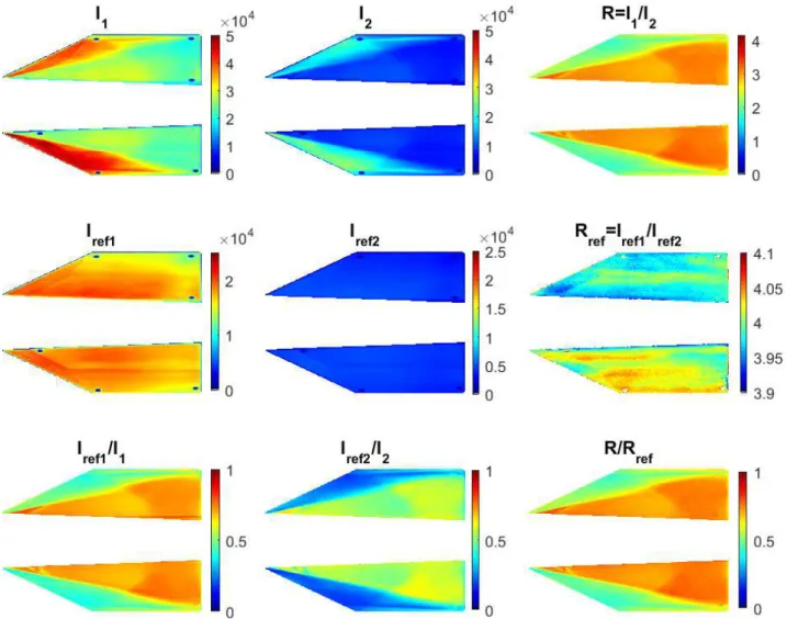
The efficiency of the lifetime ratio compared with the intensity method is illustrated in Figure 10. Let us consider this figure row by row. The first row of images consists of a pair of wind-on images subtracted for the dark current,
I1, I2 and their ratio R, obtained at M = 1, = 10°. The middle row of Figure 10 shows the dark-subtrated image pair
Iref1, Iref2 acquired wind-off at the same angle of attack, and their ratio Rref. The bottom row of Figure 10 contains the
ratios formed by the two images taken in the same column above it: Iref1/I1, Iref2/I2 and R/Rref respectively.
Very similar results were obtained for the wind-on ratio, R, the ratio I1/Iref1, comparable to the intensity method,
and the ratio R/Rref. This illustrates that the information about the pressure field was captured efficiently in the
wind-on ratio R, with the advantage of having a built-in correctiwind-on for the excitatiwind-on and model positiwind-on changes during the run.
The intensity levels of the two images I1 and I2, depend on the pressure and on the excitation distribution. The
second image, I2, acquired after the light has been turned off, is less intense than the image acquired during the
pulse. At M = 1, = 10°, the wind-on ratio R varied between 2 and 3 roughly, and this variation was due to the pressure changes on the fins. During wind-off (second row), the wind-off ratio was 4 in average, with a +/-2% peak to peak variation (RMS = 0.006%), despite a uniform atmospheric pressure on the model. This effect was observed elsewhere, and was attributed to variations of lifetime due to self quenching.10
The value of the reference ratio was also independent of the model position, orientation and the excitation levels, as was confirmed for pitch sweep and pitch step off runs. Therefore, even if the incidence was changed wind-off, a time-average Rref was used to increase the SNR of the reference measurement.
Unfortunately, the reference ratio Rref was found to vary pixel by pixel as shown in Figure 10. The effect of the
variation of the reference lifetime ratio is not apparent at M = 1, = 10°, because the pressure variation on the model was greater than the lifetime variation wind-off. Its influence was more visible at a lower Mach numbers and a lower angle of attack, as shown in Figure 11.
The data has been acquired at M = 0.6, = 0° and processed without (left image) and with (right image) a 3D pixel by pixel correction of the reference ratio variability. Without wind-off ratio correction, the variation of the Cp on the model was not uniform between the two fins, with a difference up to 0.1 Cp peak to peak. On the other hand, the data was more uniform, across each fin, and between the fins, after the wind-off ratio was used.
Before each test with this method, a reference ratio was acquired and examined: when its variation on the model exceeded some threshold fixed by the test requirements, a pixel by pixel correction using the 3D mesh was used, as illustrated in the processing pipeline shown in Figure 7. In the following, all the images have been processed using the wind-off pixel by pixel correction.
Figure 11: Cp at M = 0.6 , = 0° without (left image) and with (right image) wind-off pixel-by-pixel correction.
B. Pitch Sweep Versus Pitch Step Data at M = 1
The effect of continuously sweeping through model incidence range has been investigated around 10° angle of attack, M = 1, by comparing the PSP sweep data with the pitch step data obtained at the same condition (see Figure 12).
When the sweep motion was too fast, the paint response time lagged, and the pressure field included information from the previous angles, particularly in the regions of high pressure gradients near the leading edge of the fins. As a result, at 9 °/sec the sweep data exhibited greater Cp in the low pressure regions (Cpsweep-step ~ 0.3). At -6 °/sec, the sweep data showed lower Cp than the step data, because the model was coming from a greater angle of attack with lower Cp values: Cpsweep-step ~ -0.15. At 3 °/sec, the difference was more uniform on the model, yet slightly positive on the location of the vortex: Cpsweep-step ~ 0.03, at the most.
Figure 12: Difference between pitch sweep and pitch step Cp at M = 1, = 10°. Same Cp scale applies to all images.
Data has been extracted along the Y = +/-75mm stations shown in Figure 12 (right image), and the result is given in Figure 13. The upper fin is labelled fin 1 and the lower fin 2. The regions of the greatest differences are the regions of the largest pressure gradient, at the limits of the leading edge vortices on the fins. This comparison showed for one of the test condition yielding the largest pressure gradients on the model, a pitch sweep motion of 3°/sec or lower was acceptable to capture accurately all the flow features on the store fins.
Figure 13: Difference between sweep and step Cp at M = 1 - = 10° along Y = +/-75mm (stations shown in Figure 12).
Another analysis of the paint response time was performed by plotting the data at two locations on the fins (X = 938 mm, and Y = +/-76 mm) versus the angle of attack. The Cp obtained for the sweep run at M = 1, was compared with the Cp obtained for the step run at the same Mach number. Only the step data averaged over the whole duration of each step (0° to 20°, by 5°) is shown in Figure 14, whereas each data point of the sweep run are displayed.
This result shows that the paint followed well the pressure changes only at the 3°/s sweep rate, and was lagging for the faster rates. These effects could not be attributed to aerodynamic hysteresis, since the measured pitch sweep lift force was independent on the various pitch rates and direction of motion, and matched the lift forces of the pitch steps.
A flow separation is noticeable in Figure 14 only on fin 2: the pressure coefficient increased for angles of attack above = 13° roughly. This was measured by both step and sweep data. This flow separation was induced by a horizontal nose strake positioned upstream of fin 2 (not visible on Figure 9), which was responsible for the flow separation at those incidences.
The Cp data was extracted at the same locations on the PSP images obtained at M = 0.80, and the comparison between step data, averaged over the step angles, and sweep data is given in Figure 15. The paint followed well the smoother pressure changes at this Mach number, for all the sweep rates. It is interesting to note that the flow separation on fin 2 starts only at about 18°.
Figure 14: Pressure coefficient at two locations on the fins (shown as white dots in the = 5°-Cp image inserted). X = 938 mm, and Y = +/-76 mm for sweep and step runs at M = 1.
Figure 15: Pressure coefficient at two locations on the fins (shown as white dots in the = 5°-Cp image inserted). X = 938 mm, and Y = +/-76 mm for sweep and step runs at M = 0.80.
C. Effect of temporal and spatial averaging at =3°/sec
T
he main drawback of the single-shot lifetime method is the low light levels that can cause a poor SNR. This reduced the pressure resolution of the method compared with the intensity method in pitch step runs. One solution to improve the quality of the data is to perform temporal averaging (average several data points together around the angle of interest). When the model is moving, the number of images used should be selected carefully, in order not to compromise the desired data accuracy. The number of images used in the averaging is expected to be a function of the flow field under study, the sweep rate and the paint response to pressure changes, and should be determined for each application.Once again, the analysis is presented here for the flow condition causing a large pressure variation on the model: M = 1, around = 10°. The Cp data has been averaged over +/-4, 8, 16 data points around = 10°, which represent +/- of 0.5°, 1°, and 2°. The visual quality of the PSP data was improved by the temporal averaging, and no improvement was visible past +/-1° averaging.
The data has been extracted along a constant X station of 938 mm, shown in Figure 16 top left image, and is presented in Figure 17. The left graph in Figure 17 shows the Cp profile without averaging at angles around 10°, and the right graph shows the effect of averaging +/-0.5° and +/-1°. The noise was reduced by +/-0.04 Cp peak to peak, without affecting significantly the accuracy of the PSP data at = 10°.
Figure 16: Effect of temporal averaging on the Cp distribution at M = 1, =10°. Line in top left image corresponds to X = 938 mm.
Figure 17: Left: Cp distribution at = 10°+/-1°, M = 1, no averaging. Right: Effect of temporal averaging around =10°+/, M = 1. Data extracted at X = 938 mm in both cases.
When no temporal averaging is available, as in the case of unsteady flows, another effective method to reduce the noise level is the use of spatial averaging. Figure 18 shows that the noise reduction using a spatial filtering of +/-5 pixels was similar to that obtained using the temporal averaging of +/-1° at a pitch rate of 3°/sec. The spatial filtering worked even in the presence of sharp pressure gradients, as visible in the Cp distribution obtained at M = 1, = 10° (the unfiltered image is the top left image of Figure 16).
Figure 18: Left: Cp distribution at M = 1, = 10°, with averaging +/-5 pixels. Right: Effect of spatial averaging along X = 938 mm (section shown on the left image). Red circle is at position Y = 48mm.
D. Comparison PSP vs CFD
The comparison between PSP and CFD was performed only using the PSP data collected at the 3°/s pitch rate. A temporal averaging of +/-8 images was used in the comparison with the CFD data. This corresponded to angle brackets = +/-1°, for the pitch angles of 0° and 10°, and = +/-0° at = 20°, the model being held still for a few seconds at 20° (around t = 13.8sec, see Figure 3).
Since no pressure tap was available during the test, the CFD data was treated as the baseline for the PSP data. In particular, the CFD data was used to compute the offset at one location on fin 1, as if it were a single pressure tap, and applied to the data on both fins for each angle of attack. The location, selected outside the regions of sharp
pressure changes, is indicated in the image of Figure 18, in the form of a red circle. This offset was computed for each CFD solution available: M = 0.6, 0.8 and 1 at = 0°, 10° and 20°.
The average offset was varying between Mach numbers from 0.08Cp at M = 1, 0.05Cp at M = 0.8, and 0.03Cp at
M = 0.6, with variations of +/-0.02Cp over the angles from 0 to 20. The resulting Cp images obtained at the three
angles of attack are given in Figure 19 (M = 0.6), Figure 20 (M = 0.8) and Figure 21 (M = 1). The Cp comparison between PSP and CFD data is excellent. It is interesting to note that at M = 1, the numerical simulation has captured the oblique shock downstream of the leading edge vortices on both fins, at both angles of attack 10° and 20°. The CFD data also predicted the non-symmetric flow between the two fins at = 20°. At this incidence, the lower fin was affected by the flow separation behind a strake located near the store nose (visible in Figure 9). The effect of the nose strake on fin 2 was visible for pitch angles above 13° roughly.
Data was extracted at the stations Y = +/-48 mm, shown as straight lines in the center-right image of Figure 21. The comparison between PSP (dotted lines) and CFD (solid lines) is presented in Figure 22, at = 10°, for all available Mach numbers. The discrepancies between the CFD predictions and the PSP measurements are located at the regions of the greatest pressure gradients. This is attributed to the relative coarseness of the computational mesh in these regions. Although the leading edge vortex is well captured by the CFD solver, the mesh requires some refinement to predict better its strength. Also, the Cp plots show that the CFD solutions tend to smear out the pressure changes, which is typical of a coarse grid when simulating flows with the large pressure gradient.
For each Mach number, the conversion to pressure of all the PSP data was performed using a single offset obtained from the average of the offsets at all angles, except = 20°, where the CFD was considered to be inaccurate. The PSP data was projected on the 3D structured grid at the pixel resolution. As a result, movies of the
CFD
PSP
=0°
=10°
=20°
CFD
PSP
=0°
=10°
=20°
CFD
PSP
=0°
=10°
=20°
Figure 22: Comparison between CFD and PSP at =10°, along station Y=48 mm (fin 1, left) and Y=-48mm (fin 2, right). Line at X = 938 mm, on fin 1, indicates where the offset was computed.
V.
Conclusions
A PSP lifetime method was used for the first time in the NRC 1.5 m wind tunnel to acquire data on a moving model at various pitch rates of +3, -6°, and +9°/sec , and various Mach numbers from M = 0.6 to M = 1. Only the upper surfaces of the horizontal fins of a GBU-38 store were painted with PSP.
Since the model was not instrumented with pressure taps, the comparisons were performed using computational simulations obtained with the Cobalt CFD flow solver. As if it was measured from a single pressure tap, a single offset from one location of the CFD data was used to correct the PSP data for the wind-on temperature variations on the model.
The PSP system was composed of an Andor Zyla 5.5 sCMOS camera operated at the maximum frame rate (49 Hz) and the UV LED Hardsoft IL-106X as the excitation source. It was shown that the wind-on ratio contains all the pressure information and could be used to produce a rapid first estimate of the surface pressure distribution.
For increased pressure resolution and accuracy, the correction of the lifetime distribution wind-off was found to be necessary. This was performed using the 3D resection of the wind-on and wind-off PSP data on a structured mesh at the resolution of the pixels. The 3D data can also be available at the nodes of the unstructured surface meshes used for CFD simulations.
The PSP data obtained during the sweep motion around = 10° was compared with step data collected at M = 1. It was shown that the paint response time followed well a pitch rate of 3°/sec. Higher pitch rates introduced a lag in the PSP response, particularly in the regions of high pressure gradients.
The SNR was considerably improved with spatial filtering +/-5 pixels or (the preferred method) temporal averaging. It was shown that averaging over +/-1° did not affect the response of the PSP at M = 1 around = 10°.
The conversion of the ratios R/Rref was performed in two steps: 1) conversion to pressure assuming T = Tref, and
2) application of an offset computed at one single location on fin 1, from the difference PSP-CFD. The comparison between CFD and PSP was excellent for all flow conditions, except for the largest angle of attack. A mesh refinement could be used to improve the quality of the CFD data around the high pressure gradients.
Future work could include the acquisition of more images per pulse to extract more information from the paint,11 and the use of faster paints to increase the model motion without affecting the accuracy of the measurement.12
Acknowledgments
The authors would like to thank the Department of National Defence for providing the GBU-38 model. The first author would like to acknowledge the financial support of the NRC Aeronautical Product Development Technologies program.
References
1Bell J.H., “Pressure-Sensitive Paint Measurements on the NASA Common Research Model in the NASA 11-ft Transonic Wind Tunnel”, 49th AIAA Aerospace Sciences Meeting, Orlando, 2011, AIAA paper 2011-1128. 2Juliano T.J., Kumar P., Peng D., Gregory J.W., Crafton J. and Fonov S., “Single-shot, lifetime-based
pressure-sensitive paint for rotating blades”, Meas. Sci. Technol., 22, 085403, 2001. 3
http://www.andor.com/learning-academy/piv-mode-for-neo-and-zyla-particle-imaging-velocimetry 4
Bell J.H. et al., “Surface pressure measurements using luminescent coatings”, Annu. Rev. Fluid Mech. 33, 2001, 155-206.
5Mebarki Y., Lascombes B., Ferracina L. and Underwood J.C., “Development of Pressure-Sensitive Paints for Flexible Parachutes”, 23rd
AIAA Aerodynamic Decelerator Systems Technology Condference, 2015, AIAA paper 2015-2168.
6Mebarki Y., Cooper K.R., Reichert T.M., “Automotive Testing with Pressure-Sensitive Paint”, Journal of Flow Visualization, 2003, Volume 6, Issue 4, pp 381-393.
7Le Sant Y., Durand A., Merienne M.C., “Image Processing Tools Used for PSP and Model Deformation Measurements”, 35th
AIAA Fluid Dynamics Confernce and Exhibit, 2005, AIAA paper 2005-5007. 8
Ansys ICEM CFD - http://resource.ansys.com/Products/Other+Products/ANSYS+ICEM+CFD 9
Cobalt - http://www.cobaltcfd.com
10Bell J.H., “Accuracy limitations of lifetime-based pressure-sensitive paint (PSP) measurements”, 19th Int. Congr.
on Instrumentation in Aerospace Simulation Facilities, 2001, pp 5-16.
11Mitsuo K., Asai K., Takahashi A., and Mizushima H., “Advanced lifetime PSP imaging system for pressure and temperature field measurements”, Meas. Sci. Technol, 17, 2006.
12
Michou Y., Deleglise B., Lebrun F., Scolan E., Griverl A., Steiger R., Pugin R., Merienne M.C. and Le Sant Y., “Development of a nano-porous unsteady pressure sensitive paint and validation in the large transonic ONERA’s S2MA wind tunnel”, 31st AIAA Aerodynamic Measurement Technology and Ground Testing Conference, 2015, AIAA paper 2015-2408.