The contribution of spatial mass effects to plant diversity in arable fields

HAL Id: hal-02628595

https://hal.inrae.fr/hal-02628595

Submitted on 26 May 2020

HAL is a multi-disciplinary open access

archive for the deposit and dissemination of

sci-entific research documents, whether they are

pub-lished or not. The documents may come from

teaching and research institutions in France or

abroad, or from public or private research centers.

L’archive ouverte pluridisciplinaire HAL, est

destinée au dépôt et à la diffusion de documents

scientifiques de niveau recherche, publiés ou non,

émanant des établissements d’enseignement et de

recherche français ou étrangers, des laboratoires

publics ou privés.

Distributed under a Creative Commons Attribution| 4.0 International License

diversity in arable fields

Helen Metcalfe, Kirsty L. Hassall, Sébastien Boinot, Jonathan Storkey

To cite this version:

Helen Metcalfe, Kirsty L. Hassall, Sébastien Boinot, Jonathan Storkey. The contribution of spatial

mass effects to plant diversity in arable fields. Journal of Applied Ecology, Wiley, 2019, 56 (7),

pp.1560-1574. �10.1111/1365-2664.13414�. �hal-02628595�

1560  

|

Received: 26 November 2018 

|

R E S E A R C H A R T I C L E

The contribution of spatial mass effects to plant diversity in

arable fields

Helen Metcalfe

_{| Kirsty L. Hassall}

_{| Sébastien Boinot}

_{| Jonathan Storkey}

This is an open access article under the terms of the Creat ive Commo ns Attri bution License, which permits use, distribution and reproduction in any medium, provided the original work is properly cited.

© 2019 The Authors. Journal of Applied Ecology published by John Wiley & Sons Ltd on behalf of British Ecological Society

1_{Sustainable Agricultural}

Sciences, Rothamsted Research, Harpenden, Hertfordshire, UK

2_{Computational and Analytical}

Sciences, Rothamsted Research, Harpenden, UK

3_{System, INRA, CIHEAM‐IAMM, Montpellier}

SupAgro, Univ Montpellier, Montpellier, France

Correspondence

Helen Metcalfe

Email: helen.metcalfe@rothamsted.ac.uk

Funding information

Natural Environment Research Council; Biotechnology and Biological Sciences Research Council, Grant/Award Number: NE/N018125/1 LTS‐M

Handling Editor: Peter Manning

Abstract

1. In arable fields, plant species richness consistently increases at field edges. This potentially makes the field edge an important habitat for the conservation of the ruderal arable flora (or ‘weeds’) and the invertebrates and birds it supports. Increased diversity and abundance of weeds in crop edges could be owing to ei-ther a reduction in agricultural inputs towards the field edge and/or spatial mass effects associated with dispersal from the surrounding landscape.

2. We contend that the diversity of weed species in an arable field is a combination of resident species, that can persist under the intense selection pressure of regular cultivation and agrochemical inputs (typically more ruderal species), and transient species that rely on regular dispersal from neighbouring habitats (characterised by a more ‘competitive’ ecological strategy).

3. We analysed a large dataset of conventionally managed arable fields in the UK to study the effect of the immediate landscape on in‐field plant diversity and abun-dance and to quantify the contribution of spatial mass effects to plant diversity in arable fields in the context of the ecological strategy of the resulting community. 4. We demonstrated that the decline in diversity with distance into an arable field

is highly dependent on the immediate landscape, indicating the important role of spatial mass effects in explaining the increased species richness at field edges in conventionally managed fields.

5. We observed an increase in the proportion of typical arable weeds away from the field edge towards the centre. This increase was dependent on the immediate landscape and was associated with a higher proportion of more competitive spe-cies, with a lower fidelity to arable habitats, at the field edge.

6. Synthesis and applications. Conserving the ruderal arable plant community, and the invertebrates and birds that use it as a resource, in conventionally managed arable fields typically relies on the targeted reduction of fertilisers and herbicides in so‐ called ‘conservation headlands’. The success of these options will depend on the neighbouring habitat and boundary. They should be placed along margins where the potential for ingress of competitive species, that may become dominant in the

1 | INTRODUCTION

Arable field edges (defined as the first few metres of crop by Marshall & Moonen, 2002) have often been observed to support higher levels of species richness than field centres (Alignier, Petit, & Bohan, 2017; Marshall, 1989; Wilson & Aebischer, 1995). This increased weed di-versity at field edges presents a potential opportunity to support the conservation of biodiversity on farmland (Albrecht, Cambecèdes, Lang, & Wagner, 2016, Fried, Petit, Dessaint, & Reboud, 2009) and reconcile the trade‐off between biodiversity and agricultural pro-ductivity (the increase in plant diversity observed on organic farms is largely made up of species found in the cropped areas; Fuller et al., 2005). A diverse, abundant, naturally regenerated arable flora has been demonstrated to make a disproportionate contribution to supporting other trophic levels, including phytophagous insects (Storkey et al., 2013), bees (Bretagnolle & Gaba, 2015), natural ene-mies (Brooks et al., 2012; Norris & Kogan, 2000) and birds (Eraud et al., 2015; Henderson et al., 2012). However, the potential of the field edge flora to provide these resources will depend on the relative importance of two different processes that explain the increased di-versity at crop edges.

First, it is often argued that field edges represent a valuable hab-itat for arable plants exhibiting typical ruderal traits (sensu Grime, 1974) due to a decrease in the intensity of fertiliser and herbicide in-puts at the field edge (Alignier et al., 2017; Marshall & Moonen, 2002; Wilson & Aebischer, 1995). However, this is often inferred and has rarely been directly measured (Tsiouris & Marshall, 1998; Weaver, Downs, & Thomas, 2005). This distinct habitat is said to support rud-eral species that have an affinity to arable fields due to an adaptation to fertile and disturbed environments (Bourgeois et al., 2018) yet can no longer sustain populations under intensive herbicide and fertiliser pressure in the centre of the field (Fried et al., 2009; Kleijn & Van der Voort, 1997; Wagner, Bullock, Hulmes, Hulmes, & Pywell, 2017). In this scenario, the field edge also provides an opportunity for threat-ened arable plants to persist (Fried et al., 2009) as well as supporting the delivery of ecosystem services through enhanced biodiversity in agricultural landscapes (Bretagnolle & Gaba, 2015; Marshall et al., 2003; Storkey & Westbury, 2007). Conservation headlands (areas of crop at the edge of the field with reduced fertiliser and herbicide inputs) are the primary policy mechanism specifically targeted at conserving the arable flora (Albrecht et al., 2016).

Another hypothesis for the increased diversity at field edges is that they are subject to spatial mass effects or spill‐over of species from neighbouring habitats (Shmida & Wilson, 1985). Spatial mass

effects augment diversity within mosaic landscapes due to immi-gration from adjacent habitats (Kunin, 1998). Under this hypothe-sis, field edges receive the same management as the field centre but are biotically linked to the neighbouring habitat and, therefore, represent a unique habitat (Gabriel, Roschewitz, Tscharntke, & Thies, 2006; Kovar, 1992; Le Coeur, Baudry, Burel, & Thenail, 2002; Marshall & Moonen, 2002). As the agricultural landscape presents very steep transitional gradients between the intensively managed cropped area and the semi‐natural field boundary vegetation, we might expect that such spatial mass effects make a significant con-tribution to plant diversity and abundance at the edge of fields, due to the close proximity of the contrasting habitats. Under this hypothesis, the increase in plant diversity, through the addition of non‐arable plants, could be considered as a threat to both crop pro-duction and the conservation of rare arable plants in field edges, particularly if the additional species have a more competitive eco-logical strategy.

Here, we aim to determine the contribution of spatial mass ef-fects to plant diversity in arable fields, and the implications for both crop production and the conservation of farmland biodiversity in conventionally managed fields. Previous studies reporting the effect of the landscape on plant species richness, have focussed on large‐ scale landscape factors and have shown that landscape heteroge-neity or field size can affect weed species richness (Alignier et al., 2017; Gaba, Chauvel, Dessaint, Bretagnolle, & Petit, 2010; Gabriel et al., 2006; Gabriel, Thies, & Tscharntke, 2005; Poggio, Chaneton, & Ghersa, 2010; Roschewitz, Gabriel, Tscharntke, & Thies, 2005). Heterogeneous landscapes are composed of diverse habitat mosaics and so the species pool in these landscapes should be greater as the niche space within these different habitat types is broader than would be found in a homogeneous landscape. Smaller fields, with a higher edge/area ratio, have a greater probability of being colonised from these surrounding habitats. In contrast, other studies have failed to detect a significant relationship between landscape hetero-geneity and weed species richness (Alignier et al., 2017; Bohan & Haughton, 2012; Marshall, West, Kleijn, 2006).

One reason for the resulting uncertainty around the contribu-tion of spatial mass effects to plant diversity in arable fields is that spill‐over from neighbouring habitats will depend on the features of the immediate landscape, which are not captured in typically used metrics of habitat heterogeneity (e.g. the proportion of arable land in a predefined radius). Considering that plant mean dispersal distance is 50 m (Nathan, 2006) and that many plants typical of arable land-scapes are gravity‐dispersed (Benvenuti, 2007), it is likely that only

absence of herbicides, is limited. This will enhance ecosystem services delivered by the ruderal flora and reduce the risk of competitive species occurring in the crop.

K E Y W O R D S

agricultural landscape, arable fields, conservation headlands, fidelity score, field edge, plant diversity, spatial mass effects, weeds

the habitats immediately adjacent to the crop impact local species richness and the wider landscape exerts a relatively minor influence.

We present a novel analysis of the dataset from the Farm‐Scale Evaluations (FSE) of genetically modified, herbicide‐tolerant (GMHT) crops that represent the most extensive survey of biological com-munities in arable fields in the UK (Firbank et al., 2003). The data on weed communities have previously been used to analyse the im-portance of crop management, crop rotation and landscape in driv-ing variation in field‐scale plant diversity and abundance (Bohan & Haughton, 2012; Bohan et al., 2011; Heard et al., 2003). Here, we develop models of weed diversity and abundance that use previ-ously unreported data on the field boundary, margin (an established strip between the boundary and field edge), and habitat immediately neighbouring each field in the FSE. We contend that field‐scale arable plant diversity is a combination of resident species that can persist under the intense selection pressure of cultivation and ag-rochemical inputs (typical arable species), and transient species that rely on regular re‐colonisation from neighbouring habitats, charac-terised by a more ‘competitive’ ecological strategy (Figure 1). We use an objective measure of fidelity to arable habitats to determine the extent to which plant species are adapted to the arable habitat, and quantify the relative contribution of resident and transient species to a community. We also relate this measure of fidelity to indepen-dent measures of competitiveness to indicate the extent to which

spatial mass effects at field edges could pose a threat to both crop production and the conservation of ruderal habitats.

If spatial mass effects are making an important contribution to the variance in field‐scale plant diversity, we would expect: (a) a sig-nificant interaction between the decline in diversity and abundance with distance into the field and the nature of the neighbouring habi-tat and/or boundary feature, (b) an increase in fidelity to arable field habitats from the field edge to the centre, and (c) a weakening of these patterns post‐herbicide treatment, as transient species are re-moved, leaving a greater proportion of resident species that are able to persist in intensively managed fields owing to buffering from large persistent seedbanks or evolved resistance to herbicides. If spatial mass effects are important in determining field edge diversity and transient species are competitive with low fidelity to the arable en-vironment, these species will pose a threat to crop production and the conservation of farmland biodiversity.

2 | MATERIALS AND METHODS

2.1 | FSE dataset

We used data collected as part of the FSE study of GMHT crops (Firbank et al., 2003). The study covered 296 fields growing either sugar beet, maize, winter or spring oilseed rape (OSR) and ran from

F I G U R E 1   The gradient of management intensity (reduction in fertiliser/herbicide inputs) towards the field edge may account for some

increase in species richness observed at field edges. However, spatial mass effects will also contribute to the change in species richness and abundance at field edges. We hypothesise that the size of these effects is relative to the immediately adjacent habitats and field boundaries. (a) Large spatial mass effects, owing to species rich adjacent environments (e.g. managed grassland), boundaries (e.g. hedge) and margin, lead to a greater species richness and more abundance with a larger proportion of transient species in the community. In this scenario, fidelity scores, measuring the affinity of species to the arable habitat, will be lower. (b) Small spatial mass effects, owing to species poor adjacent environments (e.g. bare ground) and boundaries (e.g. water) lead to a low abundance of weeds with a reduced transient community in the field edge. Here, the resident weed community, buffered by the seedbank, will comprise the greater part and so the field edge community will be less diverse and show higher fidelity scores

2000 to 2002. Each field was split into two halves, a GMHT half and a conventionally cropped half. A wide range of metrics of agricultural biodiversity were collected (Firbank et al., 2003). The fields were spread widely across the lowlands of eastern and southern Britain (see Figure S1a) and were broadly representative of contemporary agriculture (Champion et al., 2003). Herbicide treatment was not stipulated in the experimental design for the conventional crops and it was left to farmers to implement ‘cost‐effective’ weed control using their normal farm management practice (Heard et al., 2003). We only used data from the conventionally managed treatments and removed all data from GMHT treatments from our analyses.

2.2 | Weed data

Weed counts at the species level were done in 0.25 × 0.5 m quadrats on 12 transects in each half‐field. The transects ran perpendicularly from the field edge into the crop with sampling points at 2, 4, 8, 16 and 32 m (Heard et al., 2003; see Figure S1b). Weeds were counted at two separate time points during the year of the experiment. The first count (pre‐herbicide dataset) was made after crop sowing and, where possible, prior to any post‐emergence herbicide application. The sec-ond count (post‐herbicide dataset) was done after the last herbicide application, allowing a delay period for mortality to occur. To address the limitation that the original experimental design focused on spring crops, we also considered a third count (winter wheat dataset) which was made in May–June of the year following the experiments for any fields where the growers chose to grow a winter wheat crop (Figure S2).

2.3 | In‐field and landscape factors

Information about the soil type of each field was provided by the farmers at the site selection stage and grouped into four categories: light, medium, heavy and organic (Firbank et al., 2003). Farmers also provided data on the field size.

The land adjacent to the trial field at the end of each transect was classified into broad habitat categories (Firbank et al., 2003—catego-ries from: Carey et al., 2002; UK Biodiversity Steering Group, 1998). We grouped these landscape factors into a single categorical vari-able ‘adjacent environment’ with categories including bare ground (ploughed field or urban), crop, managed grassland, natural grassland and woodland (Figure S3). Among the 3,028 transects, 885 were found to have multiple adjacent environments present and so were not included in the subsequent analysis.

Other landscape information was recorded for a 10‐m section at the field edge for each transect position (Firbank et al., 2003). These data included the presence or absence of margins (Figure S4), the width of any margin present and the types of field bound-ary features (Figure 1). We grouped the boundbound-ary attributes into a single categorical variable ‘adjacent boundary’ that could take any one of the following values: ditch, hedge or tree line, road, water course or no boundary (Figure S5). Transects found to have multiple adjacent boundaries, for example both a hedge and a ditch, were not included in the subsequent analysis to avoid rank deficiencies

in the modelling step. At this stage, a further 377 transects were removed from the dataset leaving 1,766 transects in our analyses.

2.4 | Analysis

2.4.1 | Diversity indices

For each of the three weed count datasets, we calculated the weed species richness and total weed abundance in each quadrat.

2.4.2 | Fidelity scores

Fidelity scores (F) are based on the relative observed species fre-quencies within the habitat of interest (arable fields) compared to other habitats (Equation 1, Chytrý, Tichý, Holt, & Botta‐Dukát, 2002). Fidelity scores range from −1 to +1 with positive (negative) values indicating that the species and the habitat of interest co‐ occur more (less) frequently than would be expected by chance. Larger positive values indicate a greater degree of joint fidelity. We defined the habitat of interest to be the central cropped area of ar-able fields and considered each field site in the FSE to be one plot in the habitat of interest (for the purposes of calculating this metric, we omitted the data in quadrats 2 m from the crop edge to avoid edge effects and to exclude the transient community, N_p = 268). We

used independent data from the Countryside Survey (Carey et al., 2008) to represent plots in other habitats. The Countryside Survey covered a total of 591 1 km × 1 km sample squares spread across England, Scotland and Wales, representative of the variations in the climate and geology of the three countries. The species of plant present were recorded for each plot. From these data, we excluded all plots in an arable or horticultural habitat as well as plots from non‐terrestrial habitats, leaving a total of N = 16,024 plots.

We computed a fidelity score for each of the 181 species pres-ent in the FSE dataset using Equation 1 where n is the total num-ber of plots in which the species is found (across both the FSE and Countryside Survey datasets) and n_p is the number of plots where the species is found in the habitat of interest (FSE dataset only).

For each quadrat within the FSE dataset, a community weighted mean (CWM) of fidelity scores (F_CWM) was calculated based on abun-dance data following

where i is the number of species present in the quadrat, p_i the pro-portion of the total number of individuals in the quadrat made up by species i and F_i the fidelity score for species i.

(1) F =√ N ⋅ np− n ⋅ Np n ⋅ Np⋅(N −n)⋅(N−Np) . FCWM= n ∑ i=1 piFi

2.4.3 | Species competitiveness

We took two complementary approaches to assess the relationship between fidelity and the relative competitiveness of weed species. First, we used data on the competitive index of various weed species estimated by Marshall et al. (2003) as the weed density required to give 5% crop yield loss in wheat, with a lower value indicating in-creased competitiveness. While the absolute value of the index will be specific to a given crop, and will also depend on local environ-ment, weather and manageenviron-ment, it is nevertheless a useful quan-titative measure of relative competitiveness. For the 25 species for which these data were available, that were also found in the FSE, we compared this competitive index (log values +0.1) to the fidelity score for that species to determine whether these two metrics were correlated (Pearson correlation).

In the second approach we recorded the ecological strategy (C/S/R, and all combinations thereof, where C species are compet-itors, S species are stress‐tolerators and R species are ruderals) ac-cording to Grime, Hodgson, and Hunt (2014), where available, for all species present in the FSE. These strategies are indicative of adap-tation to environments with contrasting soil fertility and disturbance with the difference between ruderals and competitors representing a contrast in competitive ability in fertile environments. We deter-mined the average fidelity score for each group and tested for signif-icant differences in fidelity score between the ecological strategies (one‐way ANOVA).

2.4.4 | Generalised linear mixed effects models

We investigated the effect of landscape and in‐field factors on weed diversity, abundance, and CWM fidelity scores using generalised lin-ear mixed effects models (GLMMs). Observations at the quadrat scale were used as the response, with sites and transects nested within sites included as random effects following the original experimental design. There was no evidence for spatial structure in any response variable and so no further correlation structure was incorporated into these random effects. Species richness and abundance were assumed to fol-low a Poisson distribution, while CWM fidelity scores were assumed to follow a normal distribution. For all responses, the canonical link function (natural logarithm for Poisson responses and identity for nor-mal responses) was used. For each Poisson response, the dispersion

parameter was estimated to account for over and under dispersion. We considered the following terms in the fixed effects model: dis-tance from field edge (natural logarithms), adjacent environment, adjacent boundary, the presence of a margin and its width, soil type, field size, and crop type. We also included the interaction between each landscape and in‐field factor with distance from the field edge. Due to high levels of imbalance between higher order factor level combinations, in particular the presence of combinations with zero counts (11 out of 157, see Table S1), higher order terms were not con-sidered in the model. Models were fitted using the method of Schall (1991) with terms fitted in the following order: distance + adjacent environment + adjacent boundary + margin/width + soil type + field size + crop type + distance:adjacent environment + distance:adjacent boundary + distance:margin/width + distance:soil type + distance:field size + distance:crop type. Terms were selected using backwards elimi-nation according to the largest p‐value given by an approximate F‐test when that term was dropped (Kenward & Roger, 1997). The final pre-dictive model was chosen when all remaining terms gave significant values (p ≤ 0.05) for an F test when dropped from the model.

3 | RESULTS

3.1 | Weed diversity and abundance

All three FSE datasets (pre‐herbicide, post‐herbicide and winter wheat) showed similar species richness with a mean of two to three species across all quadrats. Weed abundance was generally lower in the post‐herbicide dataset than in either the pre‐herbicide or winter wheat counts (Table 1).

3.2 | Fidelity

Of the 181 species present in the FSE dataset, the species scoring highest for fidelity were those that are typically considered as weed species with R species achieving the highest fidelity scores (Table 2). The species scoring the lowest for fidelity were mostly perennials, more commonly associated with hedgerows and grass margins, in-cluding seedlings of woody species, and were characterised by a more competitive ecological strategy. The absence of species scor-ing less than −0.1 indicates that there were no species atypical of the arable landscapes found in the dataset.

TA B L E 1   Summary statistics of diversity and abundance at the quadrat level across all three weed datasets

Diversity metric Dataset

Number of

quadrats Mean Median Min Max Lower quartile Upper quartile Variance Skew

Species richness Pre‐herbicide 7,407 2.773 2 1 16 1 4 3.387 1.419

Post‐herbicide 6,886 2.467 2 0 17 1 3 2.346 1.436

Winter wheat 3,443 2.896 2 1 15 1 4 4.458 1.639

Abundance Pre‐herbicide 7,407 14.33 6 1 491 2 16 639.4 6.376

Post‐herbicide 6,886 8.056 5 0 214 2 10 115.9 4.651

Species name Fidelity score Fidelity ranking Grimes’ eco‐ logical strategy Viola arvensis 0.560 1 R Chenopodium album 0.555 2 CR Sonchus sp. 0.513 3 R/CRa Matricaria sp. 0.501 4 Rb Fallopia convolvulus 0.498 5 R/CR Capsella bursa‐pastoris 0.492 6 R Veronica persica 0.489 7 R Lamium purpureum 0.452 8 R Urtica urens 0.434 9 R/CR Persicaria maculosa 0.402 10 R/CR Cerastium fontanum −0.043 172 R/CSR Plantago lanceolata −0.044 173 CSR Fraxinus excelsior −0.045 174 C/SC Anthriscus sylvestris −0.046 175 C/CR Urtica dioica −0.058 176 C Festuca rubra −0.066 177 CSR Agrostis stolonifera −0.071 178 CR Dactylis glomerata −0.072 179 C/CSR Rubus fruticosus −0.088 180 SC Holcus lanatus −0.088 181 CSR

a_{Strategy for Sonchus oleraceus.} b_{Strategy for Matricaria perforata (Merat).}

TA B L E 2   Fidelity scores of the species

present in the FSE dataset. Species were ranked according to their fidelity to the arable environment. Here the top and bottom ten species by their ranking are shown. The ecological strategy of these species according to Grime et al. (2014) is also shown, where C species are competitors, S species are stress tolerators and R species are ruderals

F I G U R E 2   Relationships between species competitiveness and fidelity scores. (a) Correlation between fidelity score and competitive

index (number of individuals required to give 5% crop yield loss in wheat; Marshall et al., 2003). (b) Median fidelity score for species showing different ecological strategies according to Grime et al. (2014). The relative position of the circle indicates the ecological strategy, the colour of the circle represents the median fidelity score for that ecological strategy and the number within the circle is the number of species represented by that ecological strategy

3.3 | Species competitiveness

We observed a significant correlation between the log competitive index and the fidelity score for the 25 species present in both the FSE and Marshall et al. (2003) datasets (r = 0.49, p = 0.01, Pearson correlation; Figure 2a). The correlation was positive indicating that species with low fidelity scores require fewer individuals to cause 5% yield loss and so are more competitive.

The 118 species present in our dataset for which ecological strat-egies were listed by Grime et al. (2014) comprised 14 different eco-logical strategies. Most of the species were R, R/CR or CR strategists with no S‐strategy species present within the dataset and very few S/R species (the functional group adapted to lower soil fertility that has declined because of the increased use of inorganic fertilisers; Storkey, Moss, & Cussans, 2010) (Figure 2b). There were significant differences between fidelity scores for the different ecological strat-egies (F_(13,102) = 4.58, p < 0.001) with R strategists having the high-est fidelity score. Fidelity scores generally decreased as strategies tended towards C and S types (Figure 2b, Table 2).

3.4 | Generalised linear mixed effects models

3.4.1 | Diversity and abundance

In all three datasets, there was a consistent effect of distance into the field on species richness (Table 3). In all cases, this represented an in-creased species richness at the edge of the field with lower species rich-ness at the field centre. For the pre‐herbicide dataset (Figure 3a) and winter wheat dataset (Figure S6) (both assessed prior to the application of contact herbicides), the rate of species richness decline into the field was modified, dependent on the environment in the adjacent parcel of land. Fields adjacent to grassland showed the highest level of overall spe-cies richness. The rate of decline in spespe-cies richness from the field edge to the centre was steepest for fields adjacent to woodland and man-aged grasslands while there is no increase in species richness at the field edge for fields adjacent to bare ground. For the pre‐herbicide dataset, the species richness was particularly low when adjacent to bare ground. However, in winter wheat, this distinction was not observed. Soil type also significantly impacted species richness showing that the in‐field en-vironment is still very important, although fields with organic soils (which exhibit a different response to other soil types) were underrepresented in the dataset. Crop type was not a significant term explaining variance in weed diversity prior to the application of contact herbicides.

However, following the application of herbicide, the role of the adjacent environment became insignificant and instead a significant effect of the crop type was observed indicating the importance of herbicide selectivity; OSR crops supported the largest number of species, whereas maize crops had the lowest species richness (Figure 3b). There was also a small interaction between the margin's width, if present, and the distance into the field. In this case, fields with very wide margins had higher species richness at the field edge with species richness declining towards the centre to reach the same

level as in fields with a narrow margin. TA

B LE 3  Fi na l G LM M m od el t er m s a nd t he ir s ig ni fic an ce ( N S t er m i nc lu de d i n m od el b ut n ot s ig ni fic an t, * p ≤0 .0 5, * *p ≤ 0 .01 , * ** p ≤ 0. 001 ) f or a ll d iv er si ty m et ric s a nd C W M f id el ity s co re s. A s ep ar at e m od el w as f itt ed t o e ac h d at as et f or e ac h r es po ns e v ar ia te . F or m od el s f itt ed t o t he c ou nt s m ad e i n w in te r w he at , t he c ro p t yp e i nd ic at ed h er e i s t he c ro p i n t he e xp er im en ta l y ea r an d s o r ep re se nt s t he c ro p g ro w n i n t he y ea r p rio r t o t he c ou nt Di ver si ty m et ri c D at as et M ain e ff ec ts In te ra ct io n w ith d is ta nc e i nt o t he f ie ld Di st an ce in to cro p A dja ce nt en vi ro nm en t A dja ce nt bo un da ry M ar gi n pr es en ce M ar gi n W idt h So il ty pe Fi eld si ze C ro p ty pe A dja ce nt En vi ro nm en t A dja ce nt bo un da ry M ar gi n pr es en ce M ar gi n W idt h So il ty pe Fie ld si ze C ro p t ype Sp ec ies rich ne ss Pr e‐ he rbic id e *** N S N S *** *** Po st ‐h er bi cid e *** N S N S *** N S * W in te r w he at *** *** N S ** ** *** ** A bun da nc e Pr e‐ he rbic id e *** *** *** N S N S *** ** ** N S *** Po st ‐h er bi cid e *** N S N S N S N S N S * ** *** * *** * *** W in te r w he at *** *** N S N S ** *** ** Fid el it y sc ore Pr e‐ he rbic id e *** * ** N S N S * ** *** * ** Po st ‐h er bi cid e *** N S * ** W in te r w he at *** N S N S N S N S *** ** ** *

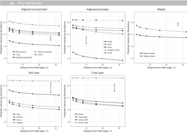
Across all three datasets many terms were selected as being important in determining overall weed abundance (Table 3) indi-cating the importance of both management (crop type) and en-vironment (soil type) as well as other landscape factors (adjacent environment, adjacent boundary, margin presence and width). In both the pre‐ and post‐herbicide counts, weed abundance dif-fered significantly according to crop type with more individuals

counted in OSR crops (Figure 4). Both before and after herbicide application, fields adjacent to bare ground had the lowest weed abundance and fields next to grassland the highest (Figure 4). In winter wheat, abundance was particularly high at the field edge in fields adjacent to grassland (Figure S7). Weed abundance also significantly varied with different boundary types although the response was not consistent across all three datasets (Figure 4,

F I G U R E 3   Predicted natural log species richness from a GLMM on (a) the pre‐herbicide dataset and (b) post‐herbicide dataset.

Model terms are shown in Table 3. Predictions are classified by distance from field edge and the main effects included in the final model. Predictions are averaged over all other terms included in the model. Error bar shows the approximate average standard error of difference

(a)

Pre-herbicide

Figure S7). Fields adjacent to roads or farm tracks had the greatest weed abundance prior to herbicide application with high abun-dance of weeds at all distances into the field.

3.4.2 | CWM fidelity scores

The CWM fidelity scores increased towards the field centre (Figure 5). This indicates that species present in the centre of the field are those more typical of arable habitats (resident species) while those present at the edge of the field are more likely to originate from other habi-tats (transient species). As well as having higher abundance, fields neighbouring grassland also had plant communities with the high-est fidelity to arable habitats indicating that species originating from grassland were most likely to be able to colonise arable fields. Prior to herbicide application (pre‐herbicide and winter wheat datasets), the adjacent boundary feature showed a significant interaction with distance into the field indicating that the way in which CWM fidelity scores changed from the field edge to the centre was modified by the boundary feature (Figure 5, Figure S8). Fields adjacent to a wa-tercourse had communities with the lowest fidelity scores and the steepest gradient in CWM fidelity score from the field edge to the

centre, whereas fields with no boundary features tended to show little change in fidelity between the field edge and centre.

Following the application of herbicide, the difference in fidelity score at the field edge was largely driven by the presence of a margin and the distance into the field. At the field centres, fidelity scores were generally high with communities composed of ‘arable species’. When there was no margin this stayed the same from the field cen-tre to the edge, yet when there was a margin present, the fidelity scores dropped at the field edge indicating that a proportion of the individuals colonising the cultivated field from the margin were able to persist following the application of contact herbicide.

4 | DISCUSSION

Our results confirm the importance of the immediate landscape in influencing the increased weed diversity and abundance observed at field edges. This provides evidence for the hypothesis that spatial mass effects contribute significantly to in‐field plant diversity and abundance and that weed communities are composed of both resi-dent weed communities, replenished by the in‐field seed bank and

FI G U R E 4 Predicted natural log abundance from a GLMM on (a) the pre‐herbicide dataset and (b) post‐herbicide dataset. Model terms are

shown in Table 3. Predictions are classified by natural logarithms of distance into field and all main effects included in the final model. Predictions are averaged over all levels of other terms included in the model. Error bar shows the approximate average standard error of difference

transient communities, which rely on repeated colonisation of field edges. We demonstrated that the spatial distribution of species rich-ness at the field scale, namely a decline in diversity with distance into the field, is highly dependent on the immediate landscape context. This confirms our first hypothesis that there is a significant interac-tion between the decline in diversity with distance into the field and the nature of the neighbouring habitat and/or boundary feature.

The highest species richness and abundance prior to the applica-tion of contact herbicides was observed in fields adjacent to grass-lands. This is indicative of grassland species having high potential to colonise arable fields and is also reflected in the relatively high CWM fidelity scores for fields neighbouring grassland. This was in contrast to the low species richness observed in fields adjacent to bare ground (including urban) where there is a limited source of new species in the local environment. Notably for the 135 transects next to bare ground, no decline with distance into the field was observed, implying that spatial mass effects may be exclusively responsible for the increased species richness at the edges of intensively managed fields.

It is interesting to note the differences between managed and natural grassland systems in terms of their effect on the total weed abundance as well as the gradient of species richness in the adjacent crop. In the pre‐herbicide dataset, we observed more species overall

and a steeper gradient in species richness from managed grasslands to the field centres, whereas the gradient from natural grassland to the field centres was shallower (although this difference was not seen in the winter wheat dataset). Natural grasslands, which gener-ally have lower soil fertility, largely consist of relatively less competi-tive stress‐tolerant species (characterised by a slow growth rate and low specific leaf area) that are likely to be less well adapted to the highly fertilised cropped field edge (DeVries et al., 2012). The prev-alence of vegetative regeneration traits in natural grasslands and greater amounts of seed dispersal in managed grasslands (Pakeman, 2004) also helps to explain the higher spatial mass effects from man-aged grasslands.

Our second hypothesis that we would see an increase in fidelity to arable field habitats from the field edge to the centre was also confirmed by our analyses indicating that transient communities at the field edge are less typical of the arable environment, whereas it is the resident communities, comprising typical arable species, that are found at the field centre. The steepest declines in diversity were observed next to woodland, which would act as a source of species poorly adapted to disturbed arable fields—a conclusion also sup-ported by the low fidelity scores observed in these transects. The idea that field boundaries are acting both as an additional source for spatial mass effects and as a barrier to dispersal is also supported by (b)

Post-herbicide

our analysis of fidelity scores, as fields adjacent to water have the lowest abundance and communities with the lowest fidelity scores possibly due to the large difference in species composition of wet-lands compared to the arable field. The observation that the pres-ence of field margins can lead to increased abundance in the field and reduced fidelity scores indicates that they may have a similar effect as neighbouring grassland (reflecting the fact that field mar-gins in the UK are dominated by grass buffer strips). This supports

the results of Marshall (2009) who found that grass margins can be a source of grasses, such as Festuca rubra, colonising the cropped field.

The reduction in species richness post‐herbicide, and the asso-ciated reduction in the number of landscape factors explaining that species richness, supports our third hypothesis and demonstrates how the application of herbicide is effective in removing transient species (rare weeds and species ingressing from other habitats; Gaba, Gabriel, Chadœuf, Bonneu, & Bretagnolle, 2016). However, (a)

Pre-herbicide

F I G U R E 5   Predicted CWM fidelity score from a GLMM on (a) the pre‐herbicide dataset and (b) post‐herbicide dataset. Model terms

are shown in Table 3. Predictions are classified by natural logarithms of distance into field and all main effects included in the final model. Predictions are averaged over all levels of other terms included in the model. Error bar shows the approximate average SE of difference

resident weed species that are present in high numbers in the centre of fields can persist post‐herbicide application owing to buffering from large persistent seedbanks and also, possibly, evolved resis-tance to herbicides (Neve, Vila‐Aiub, & Roux, 2009). The imporresis-tance of crop type in determining species richness post‐herbicide is likely to be an artefact of herbicide efficacy and selectivity in those crops and again supports the idea that the communities present at this stage are dominated by the resident weed communities and many transient species have been effectively removed by the herbicide.

Our analysis gives strong support for the view that increased spe-cies richness at the edges of fields is largely a result of spill‐over from neighbouring habitats and that spatial mass effects are a key process explaining increased weed diversity and abundance at the edges of conventionally managed fields. The absence of any S or S/R species from our dataset or any rare weeds (on the UK Biodiversity Action Plan, 2018 list of rare species in the UK) highlights the fact that in-tensive agriculture has dramatically depleted the arable flora in much of the arable landscape and so conservation measures should be tar-geted at areas where high diversity still remains (Albrecht et al., 2016). We also found that decreasing fidelity scores (associated with the field edge) were linked to more competitive species, meaning the transient weed community is more competitive in nature, and ecologically dis-tinct from the ruderal (R) dominated resident community. This finding has important implications for how we view field edges in terms of their potential to conserve arable plant communities in conventionally managed fields. While there was evidence that the competitive tran-sient species were being effectively controlled with herbicides, if left unchecked (in the absence of herbicides) they could become problem-atic weeds—lower fidelity scores were correlated with a lower com-petitive index (fewer individuals required to give 5% yield loss).

The common weed flora has an important role in support-ing farmland biodiversity (Bretagnolle & Gaba, 2015; Marshall et al., 2003) and ruderal species have been shown to dispro-portionately provide resources for phytophagous insects as well as providing chick food (Storkey et al., 2013). The seeds of many ruderal species are also an important component in the diet of farmland birds (Eraud et al., 2015; Gaba, Collas, Powolny, Bretagnolle, & Bretagnolle, 2014). Perennial field margins pro-vide a habitat to support farmland biodiversity which may offset the habitats being lost through the conversion of semi‐natural grasslands. However, these margins do not provide an oppor-tunity for ruderal species, which require areas of natural regen-eration, to persist (Butler et al., 2009). Recommendations for conserving arable plant diversity and supporting the ecosystem services provided by the ruderal flora include reducing fertiliser and herbicide application at the field edge (Albrecht et al., 2016; Wagner et al., 2017). A land‐sparing approach where these ‘con-servation headlands’ are maintained on conventionally man-aged farms would help restore plant diversity to similar levels to those found in organic farms (Fuller et al., 2005). Our results highlight the importance of considering the neighbouring habitat and boundary when deciding where to place these options in the landscape. Where there is a danger of competitive species colo-nising a conservation headland (i.e. adjacent to managed grass-lands or margins), they could become dominant in the absence of herbicides. These more competitive species would suppress the desirable ruderal species and potentially become problematic for crop production within the field. As such, the success of these conservation measures will depend on the immediate landscape context, and the potential ingress of competitive species should (b)

Post-herbicide

be considered when deciding on their arrangement in the farm landscape and subsequent management.

ACKNOWLEDGEMENTS

This research was funded by the Natural Environment Research Council (NERC) and the Biotechnology and Biological Sciences Research Council (BBSRC) under research programme NE/ N018125/1 LTS‐M ASSIST – Achieving Sustainable Agricultural Systems. This paper was produced with the support of CESAB‐FRB as part of the activities of the DISCO‐WEED Working Group. S.B. would like to thank the Agreenium International Research School (EIR‐A) and the Direction de l'action régionale, de l'enseignement su-périeur et de l'europe (DARESE) for funding his stay at Rothamsted Research. We would like to acknowledge the CEH Land Use Group for assistance with Countryside Survey data provision.

AUTHORS’ CONTRIBUTIONS

H.M., S.B. and J.S. conceived the ideas. H.M. and K.H. designed the analysis and analysed the data. H.M. led the writing of the manu-script. All authors contributed critically to the drafts and gave final approval for publication.

DATA ACCESSIBILIT Y

FSE data for Spring OSR, winter OSR, beet and maize are avail-able via the Environmental Information Data Centre. https ://doi. org/10.5285/0023b d6e‐4dd7‐462c‐aacf‐f1308 3b054ab (Scott et al., 2012). https ://doi.org/10.5285/37a50 3da‐d75c‐4d72‐8e8b‐b11c2 fdc7d92 (Scott et al., 2012). https ://doi.org/10.5285/86cd1 a60‐ 64f1‐4087‐a9f1‐a3d8a 9f8f535 (Scott et al., 2012). https ://doi. org/10.5285/ca675 2ed‐3a22‐4790‐a86d‐afada edda082 (Scott et al., 2012). Countryside Survey data are available via the Environmental Information Data Centre https ://doi.org/10.5285/57f97 915‐8ff1‐ 473b‐8c77‐2564c bd747bc (Bunce et al., 2014).

ORCID

Helen Metcalfe https://orcid.org/0000‐0002‐2862‐0266

REFERENCES

Albrecht, H., Cambecèdes, J., Lang, M., & Wagner, M. (2016). Management options for the conservation of rare arable plants in Europe.

Botany Letters, 163(4), 389–415. https ://doi.org/10.1080/23818

107.2016.1237886

Alignier, A., Petit, S., & Bohan, D. A. (2017). Relative effects of local management and landscape heterogeneity on weed richness, den-sity, biomass and seed rain at the country‐wide level, Great Britain.

Agriculture, Ecosystems & Environment, 246, 12–20. https ://doi.

org/10.1016/j.agee.2017.05.025

Benvenuti, S. (2007). Weed seed movement and dispersal strategies in the agricultural environment. Weed Biology and Management, 7(3), 141–157. https ://doi.org/10.1111/j.1445‐6664.2007.00249.x

Bohan, D. A., & Haughton, A. J. (2012). Effects of local landscape richness on in‐field weed metrics across the Great Britain scale. Agriculture,

Ecosystems & Environment, 158, 208–215. https ://doi.org/10.1016/j.

agee.2012.03.010

Bohan, D. A., Powers, S. J., Champion, G., Haughton, A. J., Hawes, C., Squire, G., … Mertens, S. K. (2011). Modelling rotations: Can crop se-quences explain arable weed seedbank abundance? Weed Research,

51(4), 422–432. https ://doi.org/10.1111/j.1365‐3180.2011.00860.x

Bourgeois, B., Munoz, F., Fried, G., Mahaut, L., Armengot, L., Denelle, P., … Violle, C. (2018). What makes a weed a weed? A large‐scale evalu-ation of arable weeds through a functional lens. American Journal of

Botany, 106(1), 90–100. in press.

Bretagnolle, V., & Gaba, S. (2015). Weeds for bees? A Review. Agronomy

for Sustainable Development, 35(3), 891–909. https ://doi.org/10.1007/

s13593‐015‐0302‐5

Brooks, D. R., Storkey, J., Clark, S. J., Firbank, L. G., Petit, S., & Woiwod, I. P. (2012). Trophic links between functional groups of arable plants and beetles are stable at a national scale. Journal of Animal Ecology, 1, 4–13. https ://doi.org/10.1111/j.1365‐2656.2011.01897.x

Bunce, R. G. H., Carey, P. D., Maskell, L. C., Norton, L. R., Scott, R. J., Smart, S. M., & Wood, C. M. (2014). Countryside Survey 2007 vege-tation plot data. NERC Environmental Information Data Centre. Butler, S. J., Brooks, D., Feber, R. E., Storkey, J., Vickery, J. A., & Norris, K.

(2009). A cross‐taxonomic index for quantifying the health of farm-land biodiversity. Journal of Applied Ecology, 46(6), 1154–1162. https ://doi.org/10.1111/j.1365‐2664.2009.01709.x

Carey, P. D., Barnett, C. L., Greenslade, P. D., Hulmes, S., Garbutt, R. A., Warman, E. A., … Firbank, L. G. (2002). A comparison of the ecologi-cal quality of land between an English agri‐environment scheme and the countryside as a whole. Biological Conservation, 108(2), 183–197. https ://doi.org/10.1016/S0006‐3207(02)00105‐2

Carey, P. D., Wallis, S., Chamberlain, P. M., Cooper, A., Emmett, B. A., Maskell, L. C., …Ullyett, J. M. (2008)Countryside Survey: UK Results from 2007. NERC/Centre for Ecology & Hydrology, 105 pp. (CEH Project Number: C03259).

Champion, G. T., May, M. J., Bennett, S., Brooks, D. R., Clark, S. J., Daniels, R. E., … Thomas, M. R. (2003). Crop management and agronomic context of the Farm Scale Evaluations of genetically modified herbi-cide–tolerant crops. Philosophical Transactions of the Royal Society B:

Biological Sciences, 358(1439), 1801–1818. https ://doi.org/10.1098/

rstb.2003.1405

Chytrý, M., Tichý, L., Holt, J., & Botta‐Dukát, Z. (2002). Determination of diagnostic species with statistical fidelity mea-sures. Journal of Vegetation Science, 13(1), 79–90. https ://doi. org/10.1111/j.1654‐1103.2002.tb020 25.x

De Vries, F. T., Manning, P., Tallowin, J. R. B., Mortimer, S. R., Pilgrim, E. S., Harrison, K. A., … Bardgett, R. D. (2012). Abiotic drivers and plant traits explain landscape‐scale patterns in soil micro-bial communities. Ecology Letters, 15(11), 1230–1239. https ://doi. org/10.1111/j.1461‐0248.2012.01844.x

Eraud, C., Cadet, E., Powolny, T., Gaba, S., Bretagnolle, F., & Bretagnolle, V. (2015). Weed seeds, not grain, contribute to the diet of win-tering skylarks in arable farmlands of Western France. European

Journal of Wildlife Research, 61(1), 151–161. https ://doi.org/10.1007/

s10344‐014‐0888‐y

Firbank, L. G., Heard, M. S., Woiwod, I. P., Hawes, C., Haughton, A. J., Champion, G. T., … Perry, J. N. (2003). An introduction to the Farm‐Scale Evaluations of genetically modified herbicide‐tol-erant crops. Journal of Applied Ecology, 40(1), 2–16. https ://doi. org/10.1046/j.1365‐2664.2003.00787.x

Fried, G., Petit, S., Dessaint, F., Reboud, X. (2009). Arable weed decline in Northern France: Crop edges as refugia for weed conservation?

Biological Conservation, 142(1), 238–243.

Fuller, R. J., Norton, L. R., Feber, R. E., Johnson, P. J., Chamberlain, D. E., Joys, A. C., … Firbank, L. G. (2005). Benefits of organic farming to

biodiversity vary among taxa. Biology Letters, 1, 431–434. https :// doi.org/10.1098/rsbl.2005.0357

Gaba, S., Chauvel, B., Dessaint, F., Bretagnolle, V., & Petit, S. (2010). Weed species richness in winter wheat increases with landscape heteroge-neity. Agriculture, Ecosystems & Environment, 138(3–4), 318–323. Gaba, S., Collas, C., Powolny, T., Bretagnolle, F., & Bretagnolle, V. (2014).

Skylarks trade size and energy content in weed seeds to maximize total ingested lipid biomass. Behavioural Processes, 108, 142–150. https ://doi.org/10.1016/j.beproc.2014.10.004

Gaba, S., Gabriel, E., Chadœuf, J., Bonneu, F., & Bretagnolle, V. (2016). Herbicides do not ensure for higher wheat yield, but eliminate rare plant species. Scientific Reports, 6, 30112. https ://doi.org/10.1038/ srep3 0112

Gabriel, D., Roschewitz, I., Tscharntke, T., & Thies, C. (2006). Beta di-versity at different spatial scales: Plant communities in organic and conventional agriculture. Ecological Applications, 16(5), 2011–2021. https ://doi.org/10.1890/1051‐0761(2006)016[2011:BDADS S]2.0.CO;2

Gabriel, D., Thies, C., & Tscharntke, T. (2005). Local diversity of ar-able weeds increases with landscape complexity. Perspectives in

Plant Ecology, Evolution and Systematics, 7(2), 85–93. https ://doi.

org/10.1016/j.ppees.2005.04.001

Grime, J. P. (1974). Vegetation classification by reference to strategies.

Nature, 250(5461), 26. https ://doi.org/10.1038/250026a0

Grime, J. P., Hodgson, J. G., & Hunt, R. (2014). Comparative plant ecol‐

ogy: A functional approach to common British species (2nd ed). Berlin:

Springer.

Heard, M. S., Hawes, C., Champion, G. T., Clark, S. J., Firbank, L. G., Haughton, A. J., … Skellern, M. P. (2003). Weeds in fields with contrasting conventional and genetically modified herbicide–tol-erant crops. I. Effects on abundance and diversity. Philosophical

Transactions of the Royal Society B: Biological Sciences, 358(1439),

1819–1832.

Henderson, I. G., Holland, J. M., Storkey, J., Lutman, P., Orson, J., & Simper, J. (2012). Effects of the proportion and spatial arrangement of un‐cropped land on breeding bird abundance in arable rotations.

Journal of Applied Ecology, 49, 883–891.

Kenward, M. G., & Roger, J. H. (1997). Small sample inference for fixed effects from restricted maximum likelihood. Biometrics, 53, 983–997. Kleijn, D., & van der Voort, L. A. (1997). Conservation headlands for rare arable weeds: The effects of fertilizer application and light penetra-tion on plant growth. Biological Conservapenetra-tion, 81(1–2), 57–67. https :// doi.org/10.1016/S0006‐3207(96)00153‐X

Kovar, P. (1992). Ecotones in agricultural landscape. EKOLOGIA(CSFR)/

ECOLOGY(CSFR), 11(3), 251–258.

Kunin, W. E. (1998). Biodiversity at the edge: A test of the importance of spatial “mass effects” in the Rothamsted Park Grass experiments.

Proceedings of the National Academy of Sciences of the United States of America, 95(1), 207–212. https ://doi.org/10.1073/pnas.95.1.207

Le Coeur, D., Baudry, J., Burel, F., & Thenail, C. (2002). Why and how we should study field boundary biodiversity in an agrarian landscape context. Agriculture, Ecosystems & Environment, 89(1–2), 23–40. https ://doi.org/10.1016/S0167‐8809(01)00316‐4

Marshall, E. J. P. (1989). Distribution patterns of plants associated with arable field edges. Journal of Applied Ecology, 247–257. https ://doi. org/10.2307/2403665

Marshall, E. J. P. (2009). The impact of landscape structure and sown grass margin strips on weed assemblages in arable crops and their boundaries. Weed Research, 49(1), 107–115. https ://doi. org/10.1111/j.1365‐3180.2008.00670.x

Marshall, E. J. P., Brown, V. K., Boatman, N. D., Lutman, P. J. W., Squire, G. R., & Ward, L. K. (2003). The role of weeds in supporting biological diversity within crop fields. Weed Research, 43(2), 77–89. https ://doi. org/10.1046/j.1365‐3180.2003.00326.x

Marshall, E. J. P., & Moonen, A. C. (2002). Field margins in northern Europe: Their functions and interactions with agriculture. Agriculture,

Ecosystems & Environment, 89(1–2), 5–21. https ://doi.org/10.1016/

S0167‐8809(01)00315‐2

Marshall, E. J. P., West, T. M., & Kleijn, D. (2006). Impacts of an agri‐en-vironment field margin prescription on the flora and fauna of arable farmland in different landscapes. Agriculture, ecosystems & environ‐

ment, 113(1‐4), 36–44.

Nathan, R. (2006). Long‐distance dispersal of plants. Science, 313(5788), 786–788. https ://doi.org/10.1126/scien ce.1124975

Neve, P., Vila‐Aiub, M., & Roux, F. (2009). Evolutionary‐thinking in agri-cultural weed management. New Phytologist, 184(4), 783–793. https ://doi.org/10.1111/j.1469‐8137.2009.03034.x

Norris, R. F., & Kogan, M. (2000). Interactions between weeds, arthro-pod pests, and their natural enemies in managed ecosystems. Weed

Science, 48(1), 94–158. https ://doi.org/10.1614/0043‐1745(2000)04

8[0094:IBWAP A]2.0.CO;2

Pakeman, R. J. (2004). Consistency of plant species and trait re-sponses to grazing along a productivity gradient: A multi‐ site analysis. Journal of Ecology, 92(5), 893–905. https ://doi. org/10.1111/j.0022‐0477.2004.00928.x

Poggio, S. L., Chaneton, E. J., & Ghersa, C. M. (2010). Landscape com-plexity differentially affects alpha, beta, and gamma diversities of plants occurring in fencerows and crop fields. Biological Conservation,

143(11), 2477–2486. https ://doi.org/10.1016/j.biocon.2010.06.014

Roschewitz, I., Gabriel, D., Tscharntke, T., & Thies, C. (2005). The effects of landscape complexity on arable weed species diversity in organic and conventional farming. Journal of Applied Ecology, 42(5), 873–882. https ://doi.org/10.1111/j.1365‐2664.2005.01072.x

Schall, R. (1991). Estimation in generalized linear models with random effects. Biometrika, 78(4), 719–727. https ://doi.org/10.1093/biome t/78.4.719

Scott, R. J., Baker, P., Bell, D., Bennett, S., Birchall, C., Boffey, C. W. H., … Young, M. W. (2012). Farm scale evaluations of herbicide tolerant genetically modified crops. NERC Environmental Information Data Centre.

Shmida, A. V. I., & Wilson, M. V. (1985). Biological determinants of species diversity. Journal of Biogeography, 12, 1–20. https ://doi. org/10.2307/2845026

Storkey, J., Brooks, D., Haughton, A., Hawes, C., Smith, B. M., & Holland, J. M. (2013). Using functional traits to quantify the value of plant communities to invertebrate ecosystem service providers in arable landscapes. Journal of Ecology, 101(1), 38–46. https ://doi. org/10.1111/1365‐2745.12020

Storkey, J., Moss, S. R., & Cussans, J. W. (2010). Using assembly theory to explain changes in a weed flora in response to agricultural in-tensification. Weed Science, 58(1), 39–46. https ://doi.org/10.1614/ WS‐09‐096.1

Storkey, J., & Westbury, D. B. (2007). Managing arable weeds for bio-diversity. Pest Management Science, 63(6), 517–523. https ://doi. org/10.1002/ps.1375

Tsiouris, S., & Marshall, E. J. P. (1998). Observations on patterns of granu-lar fertiliser deposition beside hedges and its likely effects on the bo-tanical composition of field margins. Annals of Applied Biology, 132(1), 115–127. https ://doi.org/10.1111/j.1744‐7348.1998.tb051 89.x UK Biodiversity Action Plan, 2018UK Biodiversity Action Plan (2018).

UK BAP priority vascular plant species. Retrieved 1 October 2018, from http://jncc.defra.gov.uk/page‐5171

UK Biodiversity Steering Group (1998). Tranche 2 action plans 2. English

Nature. Peterborough, UK: Terrestrial and Freshwater Habitats.

Wagner, M., Bullock, J. M., Hulmes, L., Hulmes, S., & Pywell, R. F. (2017). Cereal density and N‐fertiliser effects on the flora and biodiversity value of arable headlands. Biodiversity and Conservation, 26(1), 85– 102. https ://doi.org/10.1007/s10531‐016‐1225‐4

Weaver, S., Downs, M., & Thomas, A. G. (2005). Weed fecundity in relation to distance from the crop edge. Field Boundary Habitats: Implications for Weed, Insect and Disease Management. Topics in

Canadian Weed Science, 1, 171–183.

Wilson, P. J., & Aebischer, N. J. (1995). The distribution of dicotyledonous arable weeds in relation to distance from the field edge. Journal of

Applied Ecology, 32, 295–310. https ://doi.org/10.2307/2405097

SUPPORTING INFORMATION

Additional supporting information may be found online in the Supporting Information section at the end of the article.

How to cite this article: Metcalfe H, Hassall KL, Boinot S,

Storkey J. The contribution of spatial mass effects to plant diversity in arable fields. J Appl Ecol. 2019;56:1560–1574.