HAL Id: hal-00416002
https://hal.archives-ouvertes.fr/hal-00416002
Submitted on 11 Sep 2009
HAL is a multi-disciplinary open access
archive for the deposit and dissemination of
sci-entific research documents, whether they are
pub-lished or not. The documents may come from
teaching and research institutions in France or
L’archive ouverte pluridisciplinaire HAL, est
destinée au dépôt et à la diffusion de documents
scientifiques de niveau recherche, publiés ou non,
émanant des établissements d’enseignement et de
recherche français ou étrangers, des laboratoires
On the regularization of singular c-optimal designs
Luc Pronzato
To cite this version:
Luc Pronzato. On the regularization of singular c-optimal designs. Mathematica Slovaca, 2009, 59
(5), pp.611-626. �hal-00416002�
On the regularization
of singular c-optimal designs
∗
Luc Pronzato
Laboratoire I3S, CNRS/Universit´e de Nice Sophia-Antipolis
Bˆat. Euclide, Les Algorithmes
BP 121, 2000 route des lucioles
06903 Sophia Antipolis cedex, France
November 26, 2008
Abstract
We consider the design of c-optimal experiments for the estimation of a scalar function h(θ) of the parameters θ in a nonlinear regression model. A c-optimal design ξ∗ may be singular, and we derive conditions
ensuring the asymptotic normality of the Least-Squares estimator of h(θ) for a singular design over a finite space. As illustrated by an example, the singular designs for which asymptotic normality holds typically depend on the unknown true value of θ, which makes singular c-optimal designs of no practical use in nonlinear situations. Some simple alternatives are then suggested for constructing nonsingular designs that approach a c-optimal design under some conditions.
Keywords. singular design, optimum design, c-optimality, D-optimality, regular asymptotic normality, consistency, LS estimation
AMS Subject Classification. 62K05, 62E20
1
Introduction
We consider experimental design for least-squares estimation in a nonlinear regression model with scalar observations
Yi= Y (xi) = η(xi, ¯θ) + εi, where ¯θ ∈ Θ , i = 1, 2 . . . (1)
where {εi} is a (second-order) stationary sequence of independent random
vari-ables with zero mean,
IE{εi} = 0 and IE{ε2i} = σ2< ∞ ∀i , (2)
Θ is a compact subset of Rp and x
i ∈ X denotes the design point
characteriz-ing the experimental conditions for the i-th observation Yi, with X a compact
subset of Rd. For the observations Y1, . . . , Y
N performed at the design points
x1, . . . , xN, the Least-Squares Estimator (LSE) ˆθNLS is obtained by minimizing
SN(θ) = N
X
i=1
[Yi− η(xi, θ)]2, (3)
with respect to θ ∈ Θ ⊂ Rp. We suppose throughout the paper that either the
xi’s are non-random constants or they are generated independently of the Yj’s
(i.e., the design is not sequential). We shall also use the following assumptions: H1η: η(x, θ) is continuous on Θ for any x ∈ X ;
H2η: ¯θ ∈ int(Θ) and η(x, θ) is two times continuously differentiable with
respect to θ ∈ int(Θ) for any x ∈ X .
Then, under H1ηthe LS estimator is strongly consistent, ˆθNLS
a.s.
→ ¯θ, N → ∞,
provided that the sequence {xi} is “rich enough”, see, e.g., [3]. For instance,
when the design points form an i.i.d. sequence generated with the probability measure ξ (which is called a randomized design with measure ξ in [7, 9]), strong consistency holds under the estimability condition
Z
X
[η(x, θ) − η(x, ¯θ)]2ξ(dx) = 0 ⇒ θ = ¯θ . (4)
Under the additional assumption H2η, ˆθNLS is asymptotically normally
dis-tributed, √
N (ˆθNLS− ¯θ)
d
→ z ∼ N (0, M−1(ξ, ¯θ)) , N → ∞ , (5) provided that the information matrix (normalized, per observation)
M(ξ, ¯θ) = 1 σ2 Z X ∂η(x, θ) ∂θ ¯ ¯ ¯ ¯¯ θ ∂η(x, θ) ∂θ> ¯ ¯ ¯ ¯¯ θ ξ(dx) (6) is nonsingular.
The paper concerns the situation where one is interested in the estimation of h(θ) rather than in the estimation of θ, with h(·) a continuous scalar function on Θ. Then, when the estimability condition (4) takes the relaxed form
Z X [η(x, θ) − η(x, ¯θ)]2ξ(dx) = 0 ⇒ h(θ) = h(¯θ) , (7) we have h(ˆθN LS) a.s.
→ h(¯θ), N → ∞. Under the assumption
Hh: h(θ) is two times continuously differentiable with respect to θ ∈ int(Θ),
assuming, moreover, that ∂h(θ)/∂θ|θ¯6= 0 and that (5) is satisfied, we also obtain
(see [5, p. 61]) √ N [h(ˆθN LS) − h(¯θ)] d → ω ∼ N µ 0,∂h(θ) ∂θ> ¯ ¯ ¯ ¯¯ θ M−1(ξ, ¯θ)∂h(θ) ∂θ ¯ ¯ ¯ ¯¯ θ ¶ , N → ∞ . (8)
In Sect. 2 we prove a similar result on the asymptotic normality of h(ˆθN
LS) when
M(ξ, ¯θ) is singular, that is, √ N [h(ˆθLSN ) − h(¯θ)] d → ω ∼ N µ 0,∂h(θ) ∂θ> ¯ ¯ ¯ ¯¯ θ M−(ξ, ¯θ)∂h(θ) ∂θ ¯ ¯ ¯ ¯¯ θ ¶ , N → ∞ , (9)
with M− a g-inverse of M. This is called regular asymptotic normality in
[9], where it is shown to hold under rather restrictive assumptions on h(·) but without requiring ˆθN
LSto be consistent. We show in Sect. 2 that when the design
space X is finite ˆθN
LS is consistent under fairly general conditions, from which
(9) then easily follows.
We use the standard approach and consider an experimental design that minimizes the asymptotic variance of h(ˆθN
LS). According to (9), this corresponds
to minimizing [∂h(θ)/∂θ>¯¯
¯
θ] M−(ξ, ¯θ) [∂h(θ)/∂θ
¯ ¯¯
θ]. Since ¯θ is unknown, local
c-optimal design is based on a nominal parameter value θ0and minimizes φ
c(ξ) = Φc[M(ξ, θ0)] with Φc(·) : M ∈ M≥→ ½ c> θ0M−cθ0 if and only if cθ0 ∈ M(M) ∞ otherwise (10)
where M≥ denotes the set of non-negative definite p × p matrices,
M(M) = {c : ∃u ∈ Rp, c = Mu} and cθ0 =∂h(θ) ∂θ ¯ ¯ ¯ ¯ θ0 .
Note that the value of Φc(M) is independent of the choice of the g-inverse M−.
Nonlinearity may be present in two places, since the model response η(x, θ) and the function of interest h(θ) may be nonlinear in θ. Local c-optimal design corresponds to c-optimal design in the linear (or more precisely linearized) model
ηL(x, θ) = fθ>0(x)θ where fθ0(x) = ∂η(x, θ)/∂θ
¯ ¯
θ0, with the linear (linearized)
function of interest hL(θ) = c>θ0θ. A design ξ∗minimizing φc(ξ) may be singular,
in the sense that the matrix M(ξ∗, θ0) is singular. In spite of an apparent
simplicity for linear models, this yields, however, a difficulty due to the fact that the function Φc(·) is only lower semi-continuous at a singular matrix M ∈ M≥.
Indeed, this property implies that lim
N →∞c >M−(ξ
N)c ≥ c>M−(ξ)c
when the empirical measure ξN of the design points converges weakly to ξ, see
e.g. [6, p. 67] and [8] for examples with strict inequality. The two types of nonlinearities mentioned above cause additional difficulties in the presence of a singular design: both ˆθN
LS and h(ˆθNLS) may not be consistent, or the asymptotic
normality (9) may not hold, see [8] for an example with a linear model and a nonlinear function h(·). It is the purpose of the paper to expose some of those difficulties and to make suggestions for regularizing a singular c-optimal design.
2
Asymptotic properties of LSE with finite X
When using a sequence of design points i.i.d. with the measure ξ, the condition (4) implies that SN(θ) given by (3) grows to infinity at rate N when θ 6= ¯θ (an
assumption used in the classic reference [3]). On the other hand, for a design sequence with associated empirical measure converging to a discrete measure ξ, this amounts to ignoring the information provided by design points x ∈ X with a relative frequency rN(x)/N tending to zero, which therefore do not appear
in the support of ξ. In order to acknowledge the information carried by such points, we can follow the same approach as in [10] from which we extract the following lemma.
Lemma 1 If for any δ > 0 lim inf N →∞ kθ−¯infθk≥δ[SN(θ) − SN(¯θ)] > 0 a.s. (11) then ˆθN LS a.s. → ¯θ as N → ∞. If for any δ > 0 Pr ½ inf kθ−¯θk≥δ[SN(θ) − SN(¯θ)] > 0 ¾ → 1 , N → ∞ , (12) then ˆθN LS p → ¯θ as N → ∞.
We can then prove the convergence of the LS estimator (in probability and a.s.) when the sumPNk=1[η(xk, θ) − η(xk, ¯θ)]2 tends to infinity fast enough for
kθ − ¯θk ≥ δ > 0 and the design space X for the xk’s is finite.
Theorem 1 Let {xi} be a design sequence on a finite set X . If DN(θ, ¯θ) =
PN k=1[η(xk, θ) − η(xk, ¯θ)]2 satisfies for all δ > 0 , · inf kθ−¯θk≥δDN(θ, ¯θ) ¸ /(log log N ) → ∞ , N → ∞ , (13) then ˆθN LS a.s. → ¯θ as N → ∞. If DN(θ, ¯θ) simply satisfies
for all δ > 0 , inf
kθ−¯θk≥δDN(θ, ¯θ) → ∞ as N → ∞ , (14)
then ˆθN LS
p
→ ¯θ, N → ∞.
Proof. The proof is based on Lemma 1. We have SN(θ) − SN(¯θ) = DN(θ, ¯θ) 1 + 2 P x∈X ³PN k=1, xk=xεk ´ [η(x, ¯θ) − η(x, θ)] DN(θ, ¯θ) ≥ DN(θ, ¯θ) 1 − 2 P x∈X ¯ ¯ ¯PNk=1, xk=xεk ¯ ¯ ¯ |η(x, ¯θ) − η(x, θ)| DN(θ, ¯θ) .
From Lemma 1, under the condition (13) it suffices to prove that sup kθ−¯θk≥δ P x∈X ¯ ¯ ¯PNk=1, xk=xεk ¯ ¯ ¯ |η(x, ¯θ) − η(x, θ)| DN(θ, ¯θ) a.s. → 0 (15)
for any δ > 0 to obtain the strong consistency of ˆθN
LS. Since DN(θ, ¯θ) → ∞ and
X is finite, only the design points such that rN(x) → ∞ have to be considered,
where rN(x) denotes the number of times x appears in the sequence x1, . . . , xN.
Define β(n) =√n log log n. From the law of the iterated logarithm,
for all x ∈ X , lim sup
rN(x)→∞ ¯ ¯ ¯ ¯ ¯ ¯ 1 β[rN(x)] N X k=1, xk=x εk ¯ ¯ ¯ ¯ ¯ ¯= σ √ 2 , almost surely . (16) Moreover, DN(θ, ¯θ) ≥ D1/2N (θ, ¯θ) p
rN(x)|η(x, ¯θ)−η(x, θ)| for any x ∈ X , so that
β[rN(x)]|η(x, ¯θ) − η(x, θ)| DN(θ, ¯θ) ≤ [log log rN(x)]1/2 DN1/2(θ, ¯θ) . Therefore, ¯ ¯ ¯PNk=1, xk=xεk ¯ ¯ ¯ |η(x, ¯θ) − η(x, θ)| DN(θ, ¯θ) ≤ ¯ ¯ ¯ ¯ ¯ PN k=1, xk=xεk β[rN(x)] ¯ ¯ ¯ ¯ ¯ [log log rN(x)]1/2 D1/2N (θ, ¯θ) ,
which, together with (13) and (16), gives (15).
When infkθ−¯θk≥δDN(θ, ¯θ) → ∞ as N → ∞, we only need to prove that
sup kθ−¯θk≥δ P x∈X ¯ ¯ ¯PNk=1, xk=xεk ¯ ¯ ¯ |η(x, ¯θ) − η(x, θ)| DN(θ, ¯θ) p → 0 (17)
for any δ > 0 to obtain the weak consistency of ˆθN
LS. We proceed as above and
only consider the design points such that rN(x) → ∞, with now β(n) =
√ n.
From the central limit theorem, for any x ∈ X , ³PNk=1, xk=xεk
´
/prN(x) →d
ωx∼ N (0, σ2) as rN(x) → ∞ and is thus bounded in probability. Also, for any
x ∈ X ,prN(x)|η(x, ¯θ) − η(x, θ)|/DN(θ, ¯θ) ≤ DN−1/2(θ, ¯θ), so that (14) implies
(17).
When the design space X is finite one can thus invoke Theorem 1 to ensure the consistency of ˆθN
LS. Regular asymptotic normality then follows for suitable
functions h(·).
Theorem 2 Let {xi} be a design sequence on a finite set X , with the property
that the associated empirical measure (strongly) converges to ξ (possibly singu-lar), that is, limN →∞rN(x)/N = ξ(x) for any x ∈ X , with rN(x) the number of
times x appears in the sequence x1, . . . , xN. Suppose that the assumptions H1η,
H2η and Hh are satisfied, with ∂h(θ)/∂θ|¯θ 6= 0, and that DN(θ, ¯θ) satisfies
(13). Then, ∂h(θ) ∂θ ¯ ¯ ¯¯ θ∈ M[M(ξ, ¯θ)] , (18) implies that h(ˆθN
LS) satisfies the regular asymptotic normality property (9), where
the choice of the g-inverse is arbitrary. Proof. Since ˆθN
LS
a.s.
→ ¯θ ∈ int(Θ), there exists N0 such that ˆθN
LS is in some
convex neighborhood of ¯θ for all N larger than N0 and, for all i = 1, . . . , p = dim(θ), a Taylor development of the i-th component of the gradient of the LS criterion (3) gives
{∇θSN(ˆθNLS)}i= 0 = {∇θSN(¯θ)}i+ {∇2θSN(βiN)(ˆθNLS− ¯θ)}i, (19)
with βN
i between ˆθNLSand ¯θ (and βiN measurable, see [3]). Using the fact that X
is finite we obtain ∇θSN(¯θ)/ √ N → v ∼ N (0, 4M(ξ, ¯d θ)) and ∇2 θSN(βiN)/N a.s. →
2M(ξ, ¯θ) as N → ∞. Combining this with (19), we get √
N c>M(ξ, ¯θ)(ˆθN LS− ¯θ)
d
→ z ∼ N (0, c>M(ξ, ¯θ)c) , N → ∞ ,
for any c ∈ Rp. Applying the Taylor formula again we can write
√ N [h(ˆθN LS) − h(¯θ)] = √ N ∂h(θ) ∂θ> ¯ ¯ ¯ ¯ αN (ˆθN LS− ¯θ)
for some αN between ˆθN
LS and ¯θ and ∂h(θ)/∂θ ¯ ¯ αN a.s. → ∂h(θ)/∂θ¯¯θ¯ as N → ∞.
When (18) is satisfied we can write ∂h(θ)/∂θ¯¯θ¯ = M(ξ, ¯θ)u for some u ∈ Rp,
which gives (9).
Notice that when M(ξ, ¯θ) has full rank the condition (18) is automatically
satisfied so that the other conditions of Theorem 2 are sufficient for the asymp-totic normality (8). The conclusion of the Theorem remains valid when DN(θ, ¯θ)
only satisfies (14) (convergence in probability of ˆθN
LS) with Θ a convex set, see,
e.g., [1, Th. 4.2.2].
3
Properties of standard regularization
Consider a regularized version of the c-optimality criterion defined by Φγ
c(M) = Φc[(1 − γ)M + γ ˜M]
with Φc(·) given by (10), γ a small positive number and ˜M a fixed nonsingular
p × p matrix of M≥. From the linearity of M(ξ, θ0) in ξ, when ˜M = M(˜ξ, θ0)
with ˜ξ nonsingular this equivalently defines the criterion φγc(ξ) = φc[(1 − γ)ξ + γ ˜ξ]
with φc(ξ) = Φc[M(ξ, θ0)]. Let ξ∗and ξ∗γ be two measures respectively optimal
for φc(·) and φγc(·). We have φc(ξ∗) ≤ φc[(1 − γ)ξγ∗+ γ ˜ξ] = φγc(ξγ∗) ≤ φc[(1 −
γ)ξ∗+ γ ˜ξ] ≤ (1 − γ)φ
c(ξ∗) + γφc(˜ξ) , where the last inequality follows from the
convexity of φc(·). Therefore,
0 ≤ φγc(ξ∗γ) − φc(ξ∗) ≤ γ[φc(˜ξ) − φc(ξ∗)]
which tends to zero as γ → 0, showing that ˆξγ = (1 − γ)ξ∗γ+ γ ˜ξ tends to be
c-optimal when γ decreases to zero.
We emphasize that c-optimality is defined for θ06= ¯θ. Let x(1), . . . , x(s)be the
support points of a c-optimal measure ξ∗, complement them by x(s+1), . . . , x(s+k)
so that the measure ˜ξ supported at x(1), . . . , x(s+k) (with, e.g., equal weight at
each point) is nonsingular. When N observations are made, to the measure (1 − γ)ξ∗+ γ ˜ξ corresponds a design that places approximately γ N /(s + k)
ob-servations at each of the points x(s+1), . . . , x(s+k). The example below shows
that the speed of convergence of c>θˆN
LS to c>θ may be arbitrarily slow when γ¯
tends to zero, thereby contradicting the acceptance of ξ∗ as a c-optimal design
for ¯θ.
Example: Consider the regression model defined by (1,2) with η(x, θ) = θ1
θ1− θ2[exp(−θ2x) − exp(−θ1x)] , X = [0, 10] and σ2 = 1. The D-optimal design measure ξ∗
D on X maximizing
log det M(ξ, θ0) for the nominal parameters θ0 = (0.7, 0.2)> puts mass 1/2 at
each of the two support points given approximately by x(1)= 1.25, x(2)= 6.60.
Figure 1 shows the set {fθ0(x) : x ∈ X } (solid line), its symmetric {−fθ0(x) :
x ∈ X } (dashed line) and their convex closure Fθ0, called the Elfving set (shaded
region), together with the minimum-volume ellipsoid containing Fθ0 (the points
of contact with Fθ0 correspond to the support points of ξ∗D).
From Elfving’s theorem [2], when x∗∈ [x(1), x(2)] the c-optimal design
min-imizing c>M−1(ξ, θ0)c with c = βf
θ0(x∗), β 6= 0, is the delta measure δx∗.
Obviously, the singular design δx∗ only allows us to estimate η(x∗, θ) and not h(θ) = c>θ.
Select now a second design point x0 6= x
∗ and suppose that when N
ob-servations are performed at the design points x1, . . . , xN, m of them coincide
with x0 and N − m with x
∗, where m/(log log N ) → ∞ with m/N → 0. Then,
for x06= 0 the conditions of Theorem 1 are satisfied. Indeed, the design space
equals {x0, x
∗} and is thus finite, and
DN(θ, ¯θ) = N X k=1 [η(xk, θ) − η(xk, ¯θ)]2 = (N − 2m)[η(x∗, θ) − η(x∗, ¯θ)]2 +m©[η(x∗, θ) − η(x∗, ¯θ)]2+ [η(x0, θ) − η(x0, ¯θ)]2 ª
−0.5 −0.4 −0.3 −0.2 −0.1 0 0.1 0.2 0.3 0.4 0.5 −3 −2 −1 0 1 2 3 x(1)=1.25 x(2)=6.60 x=0
Figure 1: Elfving set.
so that infkθ−¯θk>δDN(θ, ¯θ) ≥ mC(x0, x∗, δ), with C(x0, x∗, δ) a positive
con-stant, and infkθ−¯θk>δDN(θ, ¯θ)/(log log N ) → ∞ as N → ∞. Therefore,
al-though the empirical measure ξN of the design points in the experiment
con-verges strongly to the singular design δx∗, this convergence is sufficiently slow to
make ˆθN
LS(strongly) consistent. Moreover, for h(·) a function satisfying the
con-ditions of Theorem 2, h(ˆθN
LS) satisfies the regular asymptotic property (9). In the
present situation, this means that when ∂h(θ)/∂θ¯¯θ¯= βfθ¯(x∗) for some β ∈ R,
then√N [h(ˆθN LS) − h(¯θ)] d → ω ∼ N (0,£∂h(θ)/∂θ>M−(δ x∗, θ) ∂h(θ)/∂θ ¤ ¯ θ). This
holds for instance when h(·) = η(x∗, ·) (or is a function of η(x∗, ·)).
There is, however, a severe limitation in the application of this result in practical situations. Indeed, the direction fθ¯(x∗) for which regular asymptotic
normality holds is unknown since ¯θ is unknown. Let c be a given direction of
interest, the associated c-optimal design ξ∗ is determined for the nominal value
θ0. For instance, when c = (0, 1)> (which means that one is only interested in
the estimation of the component θ2), ξ∗= δx∗with x∗ solution of {fθ0(x)}1= 0
(see Figure 1), that is, x∗ satisfies
θ0
2 = [θ20+ θ01(θ01− θ20)x∗] exp[−(θ10− θ02)x∗] . (20)
For θ0= (0.7, 0.2)>, this gives x
∗= x∗(θ0) ' 4.28. In general, fθ¯(x∗) 6= fθ0(x∗)
to which c is proportional. Therefore, c /∈ M[M(ξ∗, ¯θ)] and regular asymptotic
normality does not hold for c>θˆN LS.
The example is simple enough to be able to investigate the limiting behavior of c>θˆN
LSby direct calculation. A Taylor development of the LS criterion SN(θ)
gives (19) where βN i
a.s.
→ ¯θ as N → ∞, i = 1, 2. Direct calculations give ∇θSN(¯θ) = −2 h√ m βmfθ¯(x0) + √ N − m γN −mfθ¯(x∗) i , ∇2θSN(¯θ) = 2 £ m f¯θ(x0)fθ¯>(x0) + (N − m) fθ¯(x∗)fθ>¯(x∗) ¤ + Op( √ m) ,
where βm= (1/
√
m)Pxi=x0εi and γN −m = (1/
√
N − m)Pxi=x∗εi are
inde-pendent random variables that tend to be distributed N (0, 1) as m → ∞ and
N − m → ∞. We then obtain, ˆ θNLS− ¯θ = 1 ∆(x∗, x0) ½ γN −m √ N − m µ {f¯θ(x0)} 2 −{f¯θ(x0)} 1 ¶ +√βm m µ −{f¯θ(x∗)}2 {f¯θ(x∗)}1 ¶¾ +op(1/ √ m) ,
where ∆(x∗, x0) = det(fθ¯(x∗), fθ¯(x0)). Therefore, √
N f>
¯
θ (x∗)(ˆθNLS− ¯θ) is
asymp-totically normal N (0, 1) whereas for any direction c not parallel to fθ¯(x∗)
and not orthogonal to fθ¯(x0), √
mc>(ˆθN
LS− ¯θ) is asymptotically normal (and
c>(ˆθN
LS− ¯θ) converges not faster than 1/
√
m). In particular,√mf>
¯
θ (x0)(ˆθLSN − ¯θ)
is asymptotically normal N (0, 1) and√m{ˆθN
LS− ¯θ}2 is asymptotically normal
N (0, {f¯θ(x∗)}21/∆2(x∗, x0)). ¤
The previous example has illustrated that letting γ tend to zero in a regular-ized c-optimal design (1−γ)ξ∗+γ ˜ξ raises important difficulties (one may refer to
[8] for an example with a linear model and a nonlinear function h(θ)). We shall therefore consider γ as fixed in what follows. It is interesting, nevertheless, to investigate the behavior of the c-optimality criterion when the regularized mea-sure (1 − γ)ξ∗+ γ ˜ξ approaches ξ∗ in some sense. Since γ is now fixed, we let
the support points of ˜ξ approach those of ξ∗. This is illustrated by continuing
the example above.
Example (continued): Place the proportion m = N/2 of the observations at x0
and consider the design measure ξγ,x0= (1 − γ)δx∗+ γδx0 with γ = 1/2. Since
the c-optimal design is δx∗, we consider the limiting behavior of c
>(ˆθN LS− ¯θ)
when N tends to infinity for x0 approaching x
∗. The nonsingularity of ξ1/2,x0
for x06= x
∗(and x06= 0) implies that
√
N c>(ˆθN
LS− ¯θ) is asymptotically normal
N (0, c>M−1(ξ
1/2,x0, ¯θ)c).
The asymptotic variance c>M−1(ξ
1/2,x0, ¯θ)c tends to infinity as x0tends to
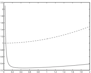
x∗ when c is not proportional to fθ¯(x∗), see Figure 2. Take c = fθ¯(x∗). Then,
f>
¯
θ (x∗)M −1(ξ
1/2,x0, ¯θ)f¯θ(x∗) equals 2 for any x0 6= x∗, twice more than what
could be achieved with the singular design δx∗since f
>
¯
θ(x∗)M −(δ
x∗, ¯θ)f¯θ(x∗) = 1
(this result is similar to that in [6, p. 67] and is caused by the fact that Φc(·) is
only semi-continuous at a singular M). ¤ The example above shows that not all regularizations are legitimate: the regularized design should be close to the optimal one ξ∗ in some suitable sense
1 1.5 2 2.5 3 3.5 4 4.5 0 1 2 3 4 5 6 Figure 2: c>M−1(ξ
1/2,x0, ¯θ)c (solid line) and fθ¯>(x∗)M−1(ξ1/2,x0, ¯θ)f¯θ(x∗)
(dashed line) for x0 varying between 1.25 and x
∗ = 4.28; ¯θ = (0.65, 0.25)>,
θ0= (0.7, 0.2)> and c = (0, 1)> (so that δ
x∗ is c-optimal for c and θ 0).
4
Minimax regularization
4.1
Estimation of a nonlinear function of θ
Consider first the case where the function of interest h(θ) is nonlinear in θ. We should then ideally take cθ¯ = ∂h(θ)/∂θ
¯ ¯¯
θ in the definition of the optimality
criterion. However, since ¯θ is unknown, a direct application of local c-optimal
design consists in using the direction cθ0 = ∂h(θ)/∂θ
¯ ¯
θ0, with the risk that θ
and h(θ) are not estimable from the associated optimal design ξ∗if it is singular.
One can then consider instead a set Θ0(a finite set or a compact subset of Rp)
of possible values for ¯θ around θ0 in the definition of the directions of interest,
and the associated c-minimax optimality criterion becomes
φC(ξ) = max θ∈Θ0c
>
θM−(ξ, θ0)cθ, (21)
or equivalently φC(ξ) = maxc∈Cc>M−(ξ, θ0)c with C = {cθ : θ ∈ Θ0}. A
measure ξ∗(C) on X that minimizes φ
C(ξ) is said to be (locally) c-minimax
optimal. When C is large enough (in particular when the vectors in C span Rp),
ξ∗(C) is nonsingular. According to Theorem 2, a design sequence on a finite set
X (containing the support of ξ∗(C)) such that the associated empirical measure
converges strongly to ξ∗(C) then ensures the asymptotic normality property (8).
4.2
Estimation of a linear function of θ: regularization via
D-optimal design
When the function of interest is h(θ) = c>θ with the direction c fixed, the
is somewhat artificial and a specific procedure is required. The rest of the section is devoted to this situation. The first approach presented is based on
D-optimality and applies when the c-optimal measure is a one-point measure.
Define a (local) c-maximin efficient measure ξ∗
mm for C as a measure on X that maximizes Emm(ξ) = min c∈C c>M−[ξ∗(c), θ0]c c>M−(ξ, θ0)c ,
with ξ∗(c) a c-optimal design measure minimizing c>M−(ξ, θ0)c. When the c-optimal design ξ∗(c) is the delta measure δ
x∗ it seems reasonable to consider
measures that are supported in the neighborhood of x∗. One may then use the
following result of Kiefer [4] to obtain a c-maximin efficient measure through
D-optimal design.
Theorem 3 A design measure ξ∗
mm on X is c-maximin efficient for CX =
{fθ0(x) : x ∈ X } if and only if it is D-optimal on X , that is, it maximizes
log det M(ξ, θ0).
The construction is as follows. Define
Xδ = B(x∗, δ) ∩ X , (22)
with B(x∗, δ) the ball of centre x∗and radius δ in Rd, and define Cδ = {fθ0(x) :
x ∈ Xδ}. From Theorem 3, a measure ξ∗δ is c-maximin efficient for c ∈ Cδ if
and only if it is D-optimal on Xδ. Suppose that Cδ spans Rp when δ > 0, the
measure ξ∗
δ is then non singular for δ > 0 (with ξ0∗= ξ∗(c)). Various values of δ
are associated with different designs ξ∗
δ. One may then choose δ by minimizing
J(δ) = max
θ∈Θ0Φc[M(ξ
∗
δ, θ)] , (23)
where Θ0 defines a feasible set for the unknown parameter vector ¯θ. Each
evaluation of J(δ) requires the determination of a D-optimal design on a set
Xδ and the determination of the minimum with respect to θ ∈ Θ0, but the
D-optimal design is often easily obtained, see the example below, and the set
Θ0 can be discretized to facilitate the determination of the maximum. Example (continued): Take c = (0 , 1)> and θ0= (0.7 , 0.2)>. Choosing X
δ as
in (22) gives Cδ = {fθ0(x) : x ∈ [x∗− δ, x∗+ δ]}, with x∗ ' 4.28, and the
cor-responding c-maximin efficient measure is ξ∗
δ = (1/2)δx∗−δ+ (1/2)δx∗+δ. Fig. 3
shows c>M−1(ξ∗
δ, ¯θ)c and fθ¯>(x∗)M−1(ξ∗δ, ¯θ)fθ¯(x∗) as functions of δ. Notice that
f>
¯
θ (x∗)M−1(ξδ∗, ¯θ)f¯θ(x∗) tends to 1 as δ tends to zero, indicating that the form
of the neighborhood used in the construction of Xδ has a strong influence on
the performance of ξ∗
δ (in terms of c-optimality) when δ tends to zero. Indeed,
taking Xδ = [x0, x∗] with x0= x∗− δ yields the same situation as that depicted
in Fig. 2.
The curve showing c>M−1(ξ∗
δ, ¯θ)c in Fig. 3 indicates the presence of a
min-imum around δ = 0.5. Fig. 4 presents J(δ) given by (23) as a function of δ when Θ0 = [0.6, 0.8] × [0.1, 0.3], indicating a minimum around δ = 1.45 (the
0 0.2 0.4 0.6 0.8 1 1.2 1.4 1.6 1.8 2 0.2 0.4 0.6 0.8 1 1.2 1.4 1.6 1.8 2 2.2 Figure 3: c>M−1(ξ∗
δ, ¯θ)c (solid line) and fθ>¯(x∗)M−1(ξδ∗, ¯θ)fθ¯(x∗) (dashed line)
for δ between 0 and 2; x∗ = 4.28, ¯θ = (0.65, 0.25)>, θ0 = (0.7, 0.2)> and
c = (0, 1)> (so that δ
x∗ is c-optimal for c and θ0).
1 1.1 1.2 1.3 1.4 1.5 1.6 1.7 1.8 1.9 2 0.44 0.46 0.48 0.5 0.52 0.54 0.56 0.58 0.6
Figure 4: maxθ∈Θ0c>M−1(ξδ∗, θ)c as a function of δ ∈ [1, 2] for Θ0= [0.6, 0.8] ×
5
Regularization by combination of c-optimal
de-signs
We say that h(θ) is locally estimable at θ for the design ξ in the regression model (1,2) if the condition (7) is locally satisfied, that is, if there exists a neighborhood Θθ of θ such that ∀θ0∈ Θ θ, Z X [η(x, θ0) − η(x, θ)]2ξ(dx) = 0 ⇒ h(θ0) = h(θ) . (24)
Consider again the case of a linear function of interest h(θ) = c>θ with the
direction c fixed. The next theorem indicates that when c>θ is not (locally)
estimable at θ0 from the c-optimal design ξ∗ it means that the support of ξ∗
depends on the value θ0 for which it is calculated. By combining different c-optimal designs obtained at various nominal values θ0,i one can thus easily
construct a nonsingular design from which θ, and thus c>θ, can be estimated.
When the true value of ¯θ is not too far from the θ0,i’s, this design will be almost c-optimal for ¯θ.
Theorem 4 Consider a linear function of interest h(θ) = c>θ, c 6= 0, in
a regression model (1,2) satisfying the assumptions H1η, H2η and Hh. Let
ξ∗= ξ∗(θ0) be a (local) c-optimal design minimizing c>M−(ξ, θ0)c. Then, h(θ) being not locally estimable for ξ∗ at θ0 implies that the support of ξ∗ varies with
the choice of θ0.
Proof. The proof is by contradiction. Suppose that the support of ξ∗(θ) does
not depend on θ. We show that it implies that h(θ) is locally estimable at θ for
ξ∗.
Suppose, without any loss of generality, that c = (c1, . . . , cp)> with c1 6= 0
and consider the reparametrization defined by β = (c>θ, θ2, . . . , θ
p)>, so that
θ = θ(β) = Jβ with J the (jacobian) matrix
J = µ 1/c1 −c0>/c1 0p−1 Ip−1 ¶ , where c0= (c2, . . . , c
p)>and 0p−1, Ip−1respectively denote the (p−1)-dimensional
null vector and identity matrix. From Elfving’s Theorem, Z S∗ ∂η(x, θ) ∂θ ξ ∗(dx) − Z Sξ∗\S∗ ∂η(x, θ) ∂θ ξ ∗(dx) = γc
with γ = γ(θ) > 0, Sξ∗ the support of ξ∗ and S∗ a subset of Sξ∗.
De-note η0(x, β) = η[x, θ(β)]. Since ∂η0(x, β)/∂β = J>∂η(x, θ)/∂θ and J>c =
(1, 0>p−1)>, we obtain Z S∗ ∂η0(x, β) ∂β ξ ∗(dx) − Z Sξ∗\S∗ ∂η0(x, β) ∂β ξ ∗(dx) = γ[θ(β)] µ 1 0p−1 ¶ .
Therefore,RS∗η0(x, β) ξ∗(dx)−
R
Sξ∗\S∗η
0(x, β) ξ∗(dx) = G(β
1), with G(β1) some
function of β1, estimable for ξ∗. Finally, β1 = c>θ is locally estimable for ξ∗
since G(β1)/dβ1= γ[θ(β)] > 0.
Example (continued): Take c = (0, 1)>, c>θ is not locally estimable at θ0 =
(0.7, 0.2)> for the c-optimal design ξ∗= δ
x∗, with x∗(θ0) ' 4.28, but the value
of x∗depends on θ0through (20). Taking two different nominal values θ0,1, θ0,2
is enough to construct a nonsingular design by mixing the associated c-optimal
designs. ¤
References
[1] H.J. Bierens. Topics in Advanced Econometrics. Cambridge University Press, Cambridge, 1994.
[2] G. Elfving. Optimum allocation in linear regression. Annals Math. Statist., 23:255–262, 1952.
[3] R.I. Jennrich. Asymptotic properties of nonlinear least squares estimation.
Annals of Math. Stat., 40:633–643, 1969.
[4] J. Kiefer. Two more criteria equivalent to D-optimality of designs. Annals
of Math. Stat., 33(2):792–796, 1962.
[5] E.L. Lehmann and G. Casella. Theory of Point Estimation. Springer, Heidelberg, 1998.
[6] A. P´azman. Foundations of Optimum Experimental Design. Reidel (Kluwer group), Dordrecht (co-pub. VEDA, Bratislava), 1986.
[7] A. P´azman and L. Pronzato. Asymptotic criteria for designs in nonlinear regression. Mathematica Slovaca, 56(5):543–553, 2006.
[8] A. P´azman and L. Pronzato. On the irregular behavior of LS estimators for asymptotically singular designs. Statistics & Probability Letters, 76:1089– 1096, 2006.
[9] A. P´azman and L. Pronzato. Asymptotic normality of nonlinear least squares under singular experimental designs. In L. Pronzato and A.A. Zhigljavsky, editors, Optimal Design and Related Areas in Optimization
and Statistics. Springer, 2008. to appear.
[10] C.F.J. Wu. Asymptotic theory of nonlinear least squares estimation. Annals


![[PDF] Apprentissage de la Conception des BD](data:image/gif;base64,R0lGODlhAQABAIAAAP///wAAACH5BAEAAAAALAAAAAABAAEAAAICRAEAOw==)