FOR INTER-WELL ESTIMATION OF POROSITY
FROM SEISMIC DATA
Muhammad M. Saggaf and M. Nafi Toksoz
Earth Resources Laboratory
Department of Earth, Atmospheric, and Planetary Sciences
Massachusetts Institute of Technology
Cambridge, MA 02139
Husam M. Mustafa
Geophysical Research and Development
Saudi Aramco
Dhahran, Saudi Arabia
ABSTRACT
We apply an approach based on smooth neural networks to a 3D seismic survey in the Shedgum area of the Ghawar Field to estimate the reservoir porosity distribution of the Arab-D Member. We conducted numerous systematic cross-validation tests to assess the accuracy of the method and to compare it to that of traditional back-propagation networks. The results obtained from these tests indicate that the regularized back-propagation network can be quite adept at estimating the porosity distribution of the reservoir in the inter-well regions from seismic data. The accuracy remained consistent as the network parameters (size and training length) were varied. On the other hand, the traditional back-propagation network gave acceptable results only when the optimal network parameters were used, and the accuracy deteriorated significantly as soon as de-viations from these optimal parameters occurred. Moreover, utilizing smooth networks, the final porosity volume corroborates our existing understanding of the reservoir and shows substantial similarity to the simple geologic model constructed by interpolating the well information, while adding significant detail and enhanced resolution to that model. We also scrutinize multi-attribute analysis, analyze how attributes can be both constructive and damaging to the prediction of the reservoir properties, and evaluate their effectiveness in enhancing the accuracy of the solution.
INTRODUCTION
Although traditional joint inversion methods have been used successfully to estimate reservoir properties from seismic data, these methods have some significant drawbacks. They require an a priori prescribed operator that links the reservoir properties to the
observed seismic response. Such operators are difficult to characterize and often hold only under ideal conditions. Furthermore, these methods rely on a linearized approach to the solution and are thus heavily dependent on the selection of the starting model. Neural networks provide a useful alternative that is inherently nonlinear and complete-ly data-driven, requiring no initial model and no explicit a priori operator linking the
measured rock properties to the seismic response. However, the performance of tradi-tional neural networks in production settings has been inconsistent due to the extensive parameter tweaking needed to achieve satisfactory results. This extensive parameter experimentation is required since these networks have a nonmonotonous generalization behavior and tend to overfit the data if the network complexity is high relative to that of the data, which makes the results of traditional networks sensitive to the network parameters (such as the size and training length).
Saggafet al. (2000) presented an approach to estimate the point-values of the
reser-voir rock properties (such as porosity) from seismic data through the use ofregularized back propagation and radial basis networks. Both types of networks have inherent smoothness characteristics that alleviate the nonmonotonous generalization problem-s aproblem-sproblem-sociated with traditional networkproblem-s and help to avert overfitting the data. That approach, therefore, avoids the drawbacks of both the joint inversion methods and tra-ditional back-propagation networks. Specifically, it is inherently nonlinear, requires no
a priori operator or initial model, and is not prone to the overfitting problems, thus
requiring no extensive parameter experimentation.
To regularize traditional back-propagation networks, their objective function is ad-justed such that the network fits the training data with the smallest network weights and offsets. This gives rise to smaller variations in the network output and yields s-moother results that are less likely to overfit the data. Other approaches that aim to alleviate the network's disposition to overfitting include redundant data interpolation (where the training data is interpolated by a smooth function prior to training) and early stopping of the network training by monitoring the errOr on a validating data set. However, Saggafet al. (2000) demonstrated that both of these approaches are less
accu-rate and less flexible than the regularization method, as the former is compute-intensive and less resistive to noise in the data, since the interpolation is carried on the noisy data and the noise is fitted faithfully. The latter approach results in a reduced training data set, which can be detrimental to network accuracy, and is also sensitive to the arbitrary split of the data available for training into training and validation subsets. The regularization method, on the other hand, does not waste valuable training data or require redundant interpolation, and its regularization parameter can be estimated automatically within the technique.
Radial basis networks achieve natural smootlmess as they perform intrinsic interpo-lation in the model space by overlapping their neural responses to the input. In terms of smoothness, radial basis networks are thus superior to traditional back-propagation networks. However, these networks are not as versatile as regularized back-propagation networks because, although they are simpler to build than their back-propagation coun-terparts, large radial basis networks are required when the training data set contains numerous input vectors. Also, the network offset, which controls the amount of smooth-ness exhibited by the network, has to be prescribed manually and the choice affects the network output significantly.
Saggaf et al. (2000) presented two architectures for setting up the input/output network geometry that are independent of the type of network utilized. Columnar architecture allows the most flexibility, since the number of output samples of the net-work is independent of that of the input, but requires the size of the input layer to be as large as the size of the input vector and thus yields very large back-propagation networks. Serialized architecture requires the number of samples of the network input and output to be the same, but the size of the resulting back-propagation network is independent of the size of the input vectorDrthe number of vectors in the training data
set, and thus produces much smaller back-propagation networks. Serialized architecture proved to be as effective as the columnar configuration when extra samples are used besides the current input sample (which enhances the vertical spatial coverage of the input) and the time index is added to the input vector (which delineates each well data set and moderates the input by adding a low frequency integrator component). Since back-propagation networks favor small but numerous input vectors while radial basis network favor few but large input vectors, serialized architecture is more appropriate for back-propagation networks while columnar architecture is more efficient with radial basis networks.
In this paper, we apply the approach described by Saggaf et al. (2000) to estimate porosity in the inter-well regions of the reservoir from seismic and well log data. The zone of interest for which we aim to predict the porosity distribution is the D Member of the Arab Formation in the Shedgum area (eastern Saudi Arabia), which is part of the Ghawar Field. The Arab Formation is comprised of four carbonate/evaporite cycles. The cycles, from top to bottom, are the A, B, C, and Arab-D Members. Individual cycles are made up of shoaling upward sequences of marine, shallow-water carbonates overlain by thick prograded marine and sabkha evaporites; the Hith Anhydrite overlies the top of the Arab Formation. Grain-supported limestone is the primary component of the Arab-D sequence, and mud-dominated limestone is more or less situated in the highly stratified lower part of the section. In some instances, dolomite replaces the Arab-D carbonates, but this is usually limited to certain intervals. Although the dolomites do not constitute a high percentage of the Arab-D rocks, they do have a profound effect on reservoir behavior. The six depositional facies identified in the Arab-D carbonates are nodular anhydrite, skeletal-oolitic, cladocoropsis, stromatoporoid-red
mainly grainstones or mud-lean packstones with high porosities, and in some cases packstones and wackestones with lower porosities.
The Arab-D reservoir itself is subdivided into five major zones: 1, 2A, 2B, 3A, and 3B. Spanning these zones are two upward shoaling depositional sequences. The lower sequence corresponds to Zone 3, while the upper sequence corresponds to Zones 1 and 2. Zone 3 is made up of a mixture of low porosity and high porosity beds. The low porosity is attributed to beds of mudstones and wackestones of the micritic lithofacies, whereas the high porosity reflects beds of grainstones and packstones of the bivalve-coated grain
intraclast lithofacies. Zones 3A and 3B were deposited on a shallow subtidal shelf. Zone
2B exhibits the entire spectrum of lithofacies types, except for nodular anhydrite, and is interpreted as an upward-shoaling sequence triggered by a major rise in sea level. The grainstones of Zone 2A consist mainly of the skeletal-oolitic lithofacies, and were interpreted to have been deposited on stable grain flats of intermediate energy that were capped by high-energy oolitic bars. In Zone 1, gradual progradation of the low energy carbonates took place over the high-energy grainstones of Zone 2A. The zone consists primarily of fully dolomitized grainstones and laminated packstones to wackestones of the skeletal-oolitic and micritic lithofacies. More detail about the depositional environ-ment of the Arab Formation is given by Powers (1962), Daetwyler and Wooten (1975), Murris (1980), and Alsharhan and Kendall (1986).
DATA DESCRIPTION AND PRE-PROCESSING
The 3D seismic data consist of 961 sublines by 441 crosslines, for a total of nearly half a million seismic traces, each sampled at 2 ms. The bin size is 25 x 25 m, and the total survey area is approximately 24 x 11 km. The data had been processed with special attention to preserving the true amplitudes, and were time migrated after stacking. Additionally, the data were filtered post-stack by the spectral compensation filter based on fractionally-integrated noise described by Saggaf and Toksiiz (1999) and Saggaf and Robinson (2000). This filtering helped to improve the event continuity, wavelet compression, and signal resolution of the data, and to attenuate persistent low frequency noise that was otherwise difficult to reduce. The top of the Arab-D zone was interpreted and the horizon was picked manually. Twenty-six milliseconds of seismic data beneath this horizon were utilized in the study, a layer that encompasses the main region of interest in this zone. Thus, each seismic trace in the survey consisted of 14 time samples.
The well log data are comprised of compensated neutron porosity logs whose tops have been carefully picked to correspond to the interpreted horizon. The logs were then converted from depth to time and resampled to the same sampling interval of the seismic data. Each well thus contributed a porosity log of 14 samples. Thirty wells in the field were utilized in the study. These wells have a somewhat good coverage of the survey area, especially at the center and south regions. The northern region and the fringes of the area have rather sparse well coverage.
For each well in the study, the converted porosity log of that well plus the nearest seismic trace to that well were used to train the network. Therefore, the training data set consisted of 30 seismic traces and 30 porosity logs, with each trace and log containing 14 samples. Further tests were carried out utilizing the nine nearest traces around each well (one at the center and eight at the perimeter of a square containing the well) instead of just a single trace. This gave rise to only a modest improvement· in the final outcome at the expense of increasing the training data set nine-fold. Therefore, we will focus only on the scheme of the single trace per well in subsequent discussions.
Preprocessing the data included mapping the seismic amplitudes to the interval
-1 to1. Mapping was performed by computing the minimum and maximum amplitudes of the training data set and then applying a linear transformation based on these values to map the seismic amplitudes. This same transformation was subsequently applied to the entire survey before it was fed into the final network. This mapping ensures that most seismic amplitudes in the survey fall within the interval to which the network transfer functions are most sensitive (Saggaf et al., 2000). Optionally, one may also apply similar mapping to the data used at the network output. This was not performed here since the output in this case is porosity, which is already nicely scaled within the region of sensitivity of the network.
Principal component analysis and discriminant factor analysis may be applied to the input data to reduce the dimension of the problem. Principal component analysis projects the original input space into a target space of lesser dimensions such that the distances between the projected points are closest to the distances in the original space. In other words, the emphasis is to minimize the distortion inflicted by the projection. Discriminant factor analysis projects the original log space into a target space of lesser dimensions such that the projected cluster centers are as far apart as possible, and so that the projected points of the same cluster are closest to each other. In other words, the emphasis is on the selection of the parameters that provide the most discrimination. We opted to forego these processes, however, as the dimension of the input vectors is already small and we did not want to inflict any unnecessary distortion on the input data representation. Anderberg (1973) and Rao (1973) give a more complete treatment of these multidimensional statistical analysis methods.
Postprocessing of the data after application of the network did not entail any special steps. However, had we scaled the porosity used in training the network, the network output would have had to be remapped from the scaled interval to the initial porosity range.
CROSS-VALIDATION RESULTS
Both the columnar and extended serialized architectures described by Saggaf et al. (2000) were utilized in our tests, and each was carried out using both regularized back-propagation and radial basis networks. As expected, the columnar architecture with the radial basis networks and the serialized architecture with the regularized
back-propagation networks required the smallest networks and gave rise to the best perfor-mance. In terms of accuracy, both the columnar and serialized architectures (the latter with three seismic samples and one depth index) gave comparable results. However, the regularized back propagation networks were in general mOre consistent and easier to utilize, since they require no manual parameter selection of the regularization parame-ter, whereas we had to experiment somewhat with the offset parameter for the radial basis networks to pick a value that gives rise to optimal smoothness. Thus, consider-ing all factors, the serialized architecture with regularized back-propagation networks proved to be the most effective, and we shall thus focus on this regime in subsequent discussions. Itremains to be seen, however, whether this scheme would be as effective in regions with extreme vertical heterogeneity. Ifit does not perform well in such cases, then the number of samples in each input vector may have to be increased to afford better vertical spatial coverage, or the columnar geometry may be used instead.
In order to gauge the accuracy of the technique, systematic cross-validations tests of the data were carried out. In each of these tests, one well is removed from the training data set. The network is trained on the remaining wells and applied on a seismic trace at that hidden well location, then the output of the network is compared to the actual porosity log of the well. The test is then repeated for each well in the training data set. This cross-validation offers an excellent measure of the accuracy of the method and provides an objective assessment of its effectiveness. We next analyze the results produced by the traditional and regularized back-propagation networks. As we mentioned previously, we shall focus this analysis on the serialized architecture. The results obtained using the columnar configuration yield similar conclusions, however.
Optimal
Network Parameters
Figure la shows a cross-plot of the predicted and measured porosity values for each well in the cross-validation study. The points belonging to each well in this plot came from a different cross-validation test where the well under investigation was hidden in that test. The network utilized here is a regularized back-propagation network with a tangent sigmoidal internal layer and a linear output layer. The optimization method used to solve for the back-propagation network weights at the training stage throughout this work is the Levenberg-Marquardt technique (Hagan and Menhaj, 1994; Foresee and Hagan, 1997). The internal layer of the network had 50 nodes. The problem geometry dictates the input layer to have four nodes (three seismic samples and a depth index) and the output layer to have a single node (porosity).
The correlation coefficient between the measured and predicted porosity values is 81%, which is an excellent result that can be considered an improvement over neural network methods that do not employ regularized networks, as the correlation coefficient reported in the work of Schuelke et al. (1997) was about 73%. Note, however, that since
the two data sets are different, these results are not directly comparable, and should serve only as a rough indicator. Figure Ib shows the mean errors between the measured and predicted porosity values for each well in the cross-validation study. The mean
prediction errors for the majority of wells are less than 4% porosity, and the overall mean prediction error for all wells is 3.7%. Both the correlation coefficient and the mean prediction errors thus indicate that regularized back-propagation networks can be quite adept at estimating the porosity distribution of the reservoir from seismic data. What makes this even more significant is that to get these results, no parameter tweak-ing whatsoever was required here, maktweak-ing regularized back-propagation networks quite suitable for use in production environments, where extensive parameter experimentation would not be feasible.
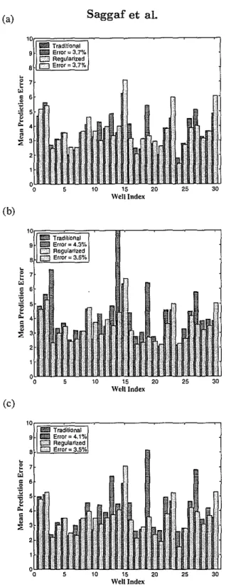
The same cannot be said for traditional back-propagation networks, however. Fig-ure 2a shows the same cross-plot previously shown in FigFig-ure la, while FigFig-ure 2b shows the corresponding result produced by a traditional back-propagation network of the same size and structure as the regularized back-propagation network discussed above. The correlation coefficient here is 79%. Figure 3a shows the same mean prediction er-rors previously shown in Figure lb, compared with those produced by the traditional back-propagation network. The overall mean prediction error for the latter is 3.7%. Comparing Figures 2a and 2b and inspecting Figure 3a seems to indicate that both the regularized and traditional networks performed equally well. This seems to hold when also comparing the correlation coefficients (81% versus 79%) and the overall mean pre-diction errors (3.7% for both). Although this may indeed seem to indicate that no improvement was gained by utilizing the regularized network, this is equivocally not the case. The reason the traditional network performed well here is that the optimal network size and training time were selected for the network after extensive experimen-tation with those parameters. As soon as deviations from these optimal parameters occur, the accuracy of the traditional network begins to deteriorate, while that of the regularized network holds steady.
Larger Network Size
We first vary the network size. Instead of using 50 nodes in the internal layer, 100 nodes are utilized. The cross-plots and correlation coefficients for the regularized and traditional networks of the same new size are shown in Figures 2c and 2d, respectively. The correlation coefficient for the regularized network has actually improved slightly (82%, up from 81%), as one would expect that a larger, more powerful network would be able to fit the intricacies of the data better. On the other hand, the correlation coefficient for the traditional network deteriorated significantly to 73% (down from 79%). Clearly, this larger network, although more powerful, has produced a rough predictive model that does not generalize well.
The same conclusion is borne in Figure 3b, which compares the mean prediction errors of the regularized and traditional networks of the larger size. We see here that the mean prediction errors for the regularized network are consistently lower than the corresponding ones for the traditional network. In fact, the overall mean prediction error for the regularized network has decreased slightly as the network became larger (3.5%, down from 3.7%), while it has significantly increased for the traditional network
(4.3%, up from 3.7%). This overall error is now 22% larger than that of the regularized network. We thus see that the accuracy of the regularized network remained consistent as the network size was increased, whereas deviating from the optimal network size adversely affected the accuracy of the traditional network to a large extent.
Longer Training Time
In the cross-validation tests discussed so far, the networks were allowed to train for 10 iterations. This is sufficient for both the regularized and traditional networks to achieve adequate convergence (in fact, it is optimal for the latter), since the Levenberg-Marquardt technique we employ in training the networks requires few iterations to converge to the solution (in contrast, the steepest descent method, for example, takes thousands of iterations to converge, although its memory requirement is smaller and each iteration requires less compute time). We next vary the training time. Instead of stopping the training after only 10 iterations, we allowed the training to continue to 50 iterations. The network size was fixed at 50 nodes in the internal layer. The corresponding cross-plots and correlation coefficients for the new regularized and tradi-tional networks are shown in Figures 2e and 2f, respectively. The correlation coefficient for the regularized network has actually increased slightly (82%, up from 81%), as we would expect that a longer training time would allow the network enough iterations to fit the data better. On the other hand, the correlation coefficient for the traditional network deteriorated to 75% (down from 79%). Clearly, as the training time increased, the network started to remember the training data set and lose its ability to generalize well.
The same conclusion can be drawn in Figure 3c, which compares the mean predic-tion errors of the regularized and tradipredic-tional networks that were allowed to train for 50 iterations. The regularized network produced consistently smaller mean prediction errors than the traditional one. As a matter of fact, the overall mean prediction er-ror for the regularized network has decreased slightly with the increased training time (3.5%, down from 3.7%), while it has significantly increased for the traditional network (4.1%, up from 3.7%). Therefore, it is evident that the accuracy of the regularized net-work remained consistent as the netnet-work was allowed to train longer, whereas deviating from the optimal training time affected the accuracy of the traditional network quite negatively.
Network Output
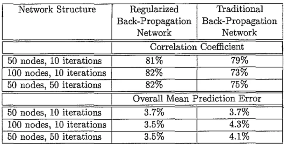
Table 1 summarizes the results discussed so far. It is evident that regularized back-propagation networks offer a much more consistent alternative to the traditional net-works, where optimal results for the latter are obtainable only with much experimenta-tion with the network parameters. These quantitative tests, however, tell only part of the story. We now inspect some examples of the actual network output.
Network Structure Regularized Traditional Back-Propagation Back-Propagation Network Network Correlation Coefficient 50 nodes, 10 iterations 81% 79% 100 nodes, 10 iterations 82% 73% 50 nodes, 50 iterations 82% 75%
Overall Mean Prediction Error
50 nodes, 10 iterations 3.7% 3.7%
100 nodes, 10 iterations 3.5% 4.3%
50 nodes, 50 iterations 3.5% 4.1%
Table 1: Summary of the results obtained by the regularized and traditional back-propagation networks for various network sizes and training lengths in the cross-validation tests that derive the porosity estimates from the seismic trace.
Figure 4a shows the porosity logs predicted for well 13 by the regularized network (solid) and traditional network (gray), as well as the measured porosity log at that well (dashed). The two networks are of the same size (50 nodes in the internal layer) and were allowed to train for 10 iterations. Even though the mean error is rather comparable in the two cases (Figure 3a), the smoothness of the output of the regularized network makes the estimated porosity more consistent and plausible, whereas the roughness of the output of the traditional network causes it to exhibit undesirable swings around the measured values. Figure 4b is similar, but for the larger, 100-node networks. We see that the output of the regularized network remains consistent and close to the measured values, while that of the traditional network overfits the data. The same observation can also be made in Figure 4c, where the measured porosity is compared to the output of the regularized and traditional networks that were allowed to train for 50 iterations. The output of the traditional network here makes such larges swings that some of the porosity values it produces (for example, between 10 and 20 ms) are considerably higher than the measured log porosity and are uncharacteristic of the reservoir in this area. Figure 5 shows the porosity values predicted for well 19. Again, the output of the regularized network remains consistent and close to the measured values regardless of the network size and training length, whereas the output of the traditional network overfits the data so severely that some of the porosity values it produces are much higher than typical in this region, or just physically impossible (for example, the negative values deeper down the well).
FINAL POROSITY DISTRIBUTION
To obtain the spatial distribution of the reservoir porosity, a final regularized back-propagation network was built using all
30
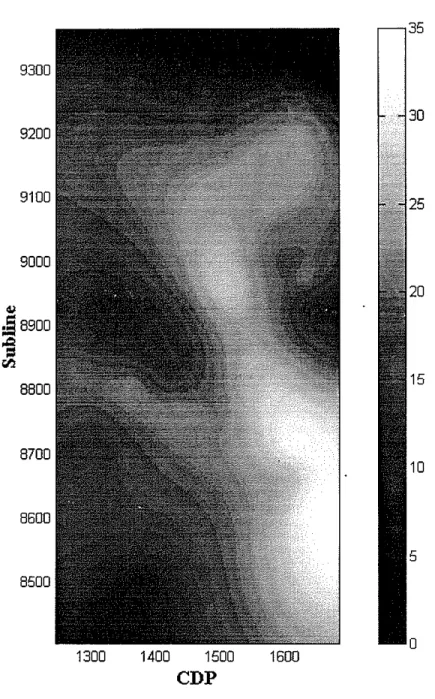
wells in the training data set (i.e., utilizing the entire training data set). This network was then applied on the whole 3D seismic survey to produce a volume that represents the porosity distribution of the reservoir. A slice of that volume is shown in Figure 6. This final porosity map is quite consistent with our existing understanding of the porosity heterogeneity of the reservoir in this region. It also corroborates the simple low frequency models that were generated by interpolating the measured porosity logs between the wells. The seismic information has added much more detail to these simple maps, however.Figure 7 shows a porosity map of the reservoir generated by interpolating the mea-sured porosity well logs with inverse-distance interpolation. Figure 8 shows a map generated by geostatistical kriging of the measured porosity well logs using a Gaussian variogram model. Figures 7 and 8 are broadly in agreement, but they differ significant-ly in the detail away from the wells, as they utilize different algorithms to perform the interpolation. In fact, even utilizing the same algorithm, these maps often differ in the details when different parameters are employed (for example, using an exponential vari-ogram model to perform the kriging instead of a Gaussian varivari-ogram model, or using the same variogram model but with different correlation lengths). This is to be expected, as these interpolation methods have no objective source of information to guide their prediction away from the wells, and hence they are quite sensitive to the interpolation algorithm and its parameters. The advantage of employing seismic information through the regularized neural network method is that the inter-well porosity estimates are much more objective and consistent, since the method utilizes an extra piece of information (seismic data) that directly samples the reservoir between the well locations. Yet, at the same time, the results obtained via this method remain in agreement with the broad picture gained from interpolated maps.
MULTI-ATTRIBUTE ANALYSIS
Seismic attribute analysis has gained a lot of momentum in recent years, and has been used extensively to aid in estimating various reservoir properties from the seismic trace. Attribute-based analyses are being applied to various aspects of reservoir exploration and development, from reservoir delineation, detection of fractures, and porosity estima-tion, to seismic structural mapping, stratigraphic analysis, lithologic characterizaestima-tion, and reservoir monitoring.
Seismic attributes extract information from the seismic data that is otherwise ob-scured or hidden and not easy to detect visually or numerically. In essence, they project the space of the seismic data on a different domain, in which the data may be more sensitive to certain reservoir properties than in the original domain. Attributes are thus able to reveal some anomalies in the data that are not easily discernible before
the transformation. This is akin to looking at an object from different views and under different lights. By varying those views and lights, one can glean features of the object that would otherwise be invisible.
Attributes originated in the work of Dennis Gabor (Gabor, 1946) and others in electrical engineering who wanted to devise ways of analyzing frequency-modulated radio signals that are not stationary in time (frequency content changes with time). By looking at the signal in both frequency and time, complex trace analysis was born. In the 1970s, Nigel Anstey, Turhan Taner, and others started looking at applying this concept to seismic data. This was the first application of seismic attributes in geophysics. Turhan Taner and Robert Sherif publicized this concept in a series of lectures in the seventies, and their work culminated in a prominent paper (Taner et al., 1979) that described the computation and application of complex seismic trace attributes. Other significant work since then has helped both broaden and refine this discipline (Robertson and Nogami, 1984; Bodine, 1986; Robertson and Fisher, 1988; Scheuer and Oldenburg, 1988; Taner et al., 1994; Brown, 1996), and the field of seismic attributes developed so quickly that recently Chen and Sidney (1997) catalogued and described over 63 attributes.
In fact, the term seismic attributes has expanded to encompass not only complex trace attributes, but also spectral, statistical, and AVO attributes as well. A popu-lar way of looking at attributes is to classify them into physical attributes that make physical sense (e.g., mass, magnitude, and phase), which are useful for lithology dis-crimination, and geometrical attributes that emphasize shape, like continuity, dip, and azimuth, which are useful for structural and stratigraphic analysis. Seismic attributes .can also be either instantaneous (local, an attribute value is calculated for each sample .in the seismic trace) or interval attributes (a value, that is an aggregate of some sort, is calculated for an entire segment of the trace), and can be single-trace attributes (derived from one trace) or multi-trace (computed from several adjacent traces).
We illustrate how seismic attributes can aid in simplifying the process of reservoir characterization with a simple example. Denote the seismic trace by x, and assume that the reservoir property under investigation is related to the seismic data by the unknown relation F(x). In order to estimate the reservoir property from the seismic data, any inversion procedure (neural networks included) must approximate the relation
F from the training data set (for neural networks, this approximation is accomplished by training the network). In other words, the solution must simulate the map:
x .... F(x). (1)
Ifthe function F is quite complex, then a very sophisticated inversion procedure (for example, a large network) would be needed to approximate it. Seismic attributes serve to reduce the complexity of the inversion process by mapping the input ofF through the extracted seismic attribute A(x) such that the resulting relation (F 0 A)(x) is a simplified version of the original relation.
actually equal toF-1
• Then all the inversion process has to determine is the map:
x -T (F0 A)(x) x -T (F0 F-1)(x) x -T x. (2) (3) (4) In this extreme case, even simple linear regression would be able to more than adequately derive the reservoir property from the extracted seismic attribute, since the resulting unknown relation to be simulated is trivial. Another advantage of seismic attributes is that they allow the interpreter to inject his own bias into the inversion process by enforcing attributes that conform to his existing notion of the reservoir, although this can certainly be a disadvantage if not used judiciously.
On the other hand, there is also the viewpoint that a careless choice of the seismic attribute utilized can actually harm the inversion process, since the resulting map to be simulated may be even more complex than the initial relation (for example, consider the case whereF itself is simple and the attributeA adds unnecessary complexity to it),
and that the extracted seismic attribute carries less information than the original trace, especially if the attribute extraction process is not reversible (de Groot and Bril, 1997). However, in practice these issues do not present a problem because (1) the attributes used usually bear some relation to the observed seismic response of the reservoir property at hand (e.g., porosity is correlated with acoustic impedance), and so the resulting map
FoAis necessarily simpler than the original model, since part of the variable dependence has already been modeled and accounted for in the attribute extraction process, and more importantly, (2) that a single attribute is seldom used in place of the raw seismic trace. In fact, multiple attributes, as well as the raw trace itself, are almost always used in union. This adds redundancy to the process and so any information lost in one space by an attribute is more than accounted for by the others. Still, indiscriminant use of numerous seismic attributes invariably leads to spurious statistical correlations (Kalkomey, 1997), and so only attributes that bear an actual physical relevance to the reservoir property under investigation should be utilized (for example, relative acoustic impedance is quite relevant to porosity).
Utilizing seismic attributes, then, can simplify the neural network design process and require less network complexity, as part of the mapping is done a priori in extracting the seismic attributes. On the other hand, since numerous attributes often need to be utilized, what these attributes achieve in reducing the network complexity is offset by requiring a large network size to accommodate this increased input. This is especially true if instantaneous, rather than average, attributes are employed. For example, in our columnar configuration, where the seismic trace consists of 14 samples and the back-propagation network has 50 nodes in its internal layer, each seismic attribute adds an extra 14 nodes to the input layer, and thus requires 700 extra network weights to be solved for at the training stage.
This problem is alleviated significantly when the serialized architecture described by Saggaf et al. (2000) is used, where each extra attribute adds only three extra input
nodes to the network. This configuration is shown in Figure 9a. In fact, since most instantaneous seismic attributes already carry information reflecting the vertical spatial continuity of the data, the extra samples at each side of the current input sample need not be used, and the network geometry is simplified even further (shown in Figure 9b). In this case, each extra seismic attribute adds only a single node to the input layer.
We used four attributes in our tests: the seismic trace itself, cosine of the instan-taneous phase (normalized amplitude), relative acoustic impedance (integrated seismic trace), and trace envelope. The neural network cross-validation process discussed in the previous section was repeated using these attributes with the simple serialized architec-ture of Figure 9b and a regularized back-propagation network of the same strucarchitec-ture and size as before (50 nodes in the internal layer). The results obtained here were equivalent to those obtained earlier but showed no significant improvement. While this is a tes-tament that the seismic attributes were indeed able to provide enough spatial coverage to account for the extra samples of the extended serialized architecture (that uses three trace samples for each porosity value (Saggaf et al., 2000)), the fact that no significant improvement in the accuracy of the network was gained even when the extended seri-alized architecture was used with the attributes (Figure gal, or, for that matter, even with the columnar architecture, seems to indicate that the regularized back-propagation network utilized in the previous section (used with only the raw seismic trace) was al-ready able to illuminate the problem sufficiently and extract the maximum amount of information from the data, such that no residual information was left to be extracted through the use of the attributes.
Itis logical to conclude, then, that the accuracy added by utilizing seismic attributes . is less significant when the underlying methodology used to perform the inversion (regu-larized neural networks in this case) is already highly powerful and inherently nonlinear.
. It seems that the increased accuracy gained by utilizing seismic attributes is inverse-ly proportional to the power of the underinverse-lying modeling process. Thus, using seismic attributes would have been much more valuable had we employed linearized inversion, linear regression, or just plain visual inspection (in increasing order of enhanced accura-cy added by the attribute analysis). We cannot say conclusively, however, that seismic attributes are not useful even with regularized neural networks; more tests (perhaps with more powerful attributes) are needed before such a conclusion can be firmly made. However, since the goal of this work is aimed at Simplifying the application of neural networks by minimizing the amount of parameter tweaking required to utilize them ef-fectively, extensive experimentation with the selection of the optimal seismic attributes seems to run against this purpose.
SUMMARY AND CONCLUSIONS
We applied the smooth neural networks approach described by Saggaf et al. (2000) to a 3D seismic survey in the Shedgum area of the Ghawar Field to estimate the reservoir porosity distribution of the Arab-D Member, the main oil producing zone of the reservoir
in this region. The training data set consisted of porosity logs of 30 wells in the area and the seismic traces nearest to those wells. The accuracy of the study was assessed though systematic cross-validations tests, and each suite of tests was repeated for both the regularized and traditional networks with various network parameters. The results of these cross-validation tests indicate that the regularized back-propagation network can be quite adept at estimating the porosity distribution of the reservoir in the inter-well regions from seismic data, as the correlation coefficient between the porosity values measured at the wells and those predicted by the regularized network was 81%. The mean prediction errors between the measured and predicted porosity were less than 4% porosity for the majority of wells in the study, with an overall average of 3.7%. Not only that, but the accuracy of the results remained consistent as the network parameters (size and training length) were varied (the accuracy actually improved slightly when those parameters were increased, as it should).
On the other hand, the traditional back-propagation network gave acceptable results only when the optimal network parameters were used. As soon as deviations from these optimal parameters occur, the accuracy of the traditional network deteriorates signifi-cantly. Increasing the network size over the optimal value Or allowing the network to train for a longer time than optimal, instead of improving the network output, actually produced a sizable decline in the accuracy of the network. The resulting output overfit the data and exhibited considerable swings around the measured values. In fact, some of these swings are so large that several of the porosity values predicted by the network are much higher than typical in this region or just physically impossible. It is eviden-t, therefore, that regularized back-propagation networks offer a much more consistent alternative to traditional networks, where optimal results for the latter are obtainable only with much experimentation with the network parameters. Utilizing regularized back-propagation networks thus eliminates the need for extensive parameter tweaking and produces networks that have much more consistent results than their traditional back-propagation counterparts. The operator need only pick a network of adequate size, there is no danger of overfitting the data if the network is too large.
The final distribution of the reservoir porosity was obtained by building a regularized back-propagation network using the entire training data set and applying that network to the whole 3D seismic survey to produce a porosity volume. This final porosity map is quite consistent with our existing understanding of the porosity heterogeneity of the reservoir in this region. Italso corroborates the simple low frequency models that were generated by interpolating the measured porosity logs between the wells, but with much enhanced detail due to the extra information added by the seismic data, which directly sample the reservoir in the inter-well regions.
Finally, although seismic attributes can be effective at illuminating the data and ex-tracting information that is otherwise obscure and not easy to detect, thus simplifying the neural network design process and requiring less network complexity since part of the mapping is done a priori in extracting the seismic attributes, the use of attributes
ex-pense of greater compute times. It seems that the regularized back-propagation network was already able to illuminate the problem sufficiently to extract the maximum amount of information from the data, such that no residual information was left to be extracted through the use of the attributes. Even though further experimentation with the se-lection of the attributes may yet prove effective in significantly improving the accuracy of the network, such extensive experimentation is in contrast to our objective of sim-plifying the application of neural networks in estimating the reservoir properties from seismic data to be conducive to more widespread use of neural networks in production settings.
ACKNOWLEDGMENTS
We would like to thank Saudi Aramco for supporting this research and for granting us permission for its publication. This work was also supported by the Borehole A-coustics and Logging/Reservoir Delineation Consortia at the Massachusetts Institute of Technology.
REFERENCES
Alsharhan, A.S. and Kendall, C.G., 1986, Precambrian to Jurassic rocks of Arabian Gulf and adjacent areas: Their facies, depositional setting, and hydrocarbon habitat, AAPG Bull., 70, 977-1002.
Anderberg, M.R, 1973, Cluster Analysis for Applications, Academic Press.
Bodine, J.H., 1986, Wave-form analysis with seismic attributes, Oil and Gas J., 84, 59-63.
Brown, A.R., 1996, Seismic attributes and their classification, The Leading Edge, 15, 1090.
Chen, Q. and Sidney, S., 1997, Seismic attribute technology for reservoir forecasting and monitoring, The Leading Edge, 16, 445-456.
Daetwyler, C.C.and Wooten, J.N., 1975, Arab-D geological reservoir description, 'Utham-niyah area, Ghawar Field, Saudi Arabia, EPR Tech. Service Rept., EPR.153ES.75. de Groot, P.F.M. and Bril, A.H., 1997, Quantitative interpretation generally needs no seismic attributes, Extended Abstracts, 59th Mtg. Eur. Assoc. Expl. Geophys., Ses-sion EOI8.
Foresee, F.D. and Hagan, M.T., 1997, Gauss-Newton approximation to Bayesian regu-larization, Proceed. 1997Internat. Joint Conf. Neural Networks, 1930--1935.
Gabor, D., 1946, Theory of communication, Part I, J. Inst. Elect. Eng., 93, 429-441. Hagan M.T. and Menhaj, M., 1994, Training feedforward networks with the Marquardt
algorithm, IEEE Trans. Neural Networks, 5, 989-993.
Kalkomey, C.T., 1997, Potential risks when using seismic attributes as predictors of reservoir properties, The Leading Edge, 16, 247-251.
Murris, RJ., 1980, Middle East: Stratigraphic evolution and oil habitat, AAPG, 64, 597-618.
Powers, RW., 1962, Arabian Upper Jurassic carbonate reservoir rocks in classification of carbonate rocks, in Ham, W.E. (Ed.), AAPG Memoir 1, 122-192.
Rao, C.R, 1973, Linear Statistical Inference and its Application, John Wiley and Sons,
NY.
Robertson, J.D. and Nogami, H.H., 1984, Complex seismic trace analysis of thin beds, Geophysics,
49,
344-352.Robertson, J.D. and Fisher, D.A., 1988, Complex seismic trace attributes, The Leading Edge, 07, 22-26.
Saggaf, M.M. and Robinson, E.A., 2000, A unified framework for the deconvolution of traces of non-white reflectivity, Geophysics, in publication.
Saggaf, M.M. and ToksDz, M.N., 1999, An analysis of deconvolution: modeling reflec-tivity by fractionally integrated noise, Geophysics,
64,
1093-1107.Saggaf, M.M., ToksDz, M.N., and Mustafa, H.M., 2000, Estimation of reservoir proper-ties from seismic data by smooth neural networks, this report, 2-1-2-36.
Scheuer, T.E. and Oldenburg, D.W., 1988, Local phase velocity from complex seismic data, Geophysics, 53, 1503-1511.
Schuelke, J.S., Quirein, J.A., Sarg, J.F., Altany, D.A. and Hunt, P.E., 1997, Reservoir architecture and porosity distribution, Pegasus field, West Texas-an integrated sequence stratigraphic-seismic attribute study using neural networks, Expanded
Abstracts, 67th Ann. Internat. Mtg., Soc. Expl. Geophys., 668-671.
Taner, M.T., Koehler, F. and Sheriff, R.E., 1979, Complex seismic trace analysis,
Geo-physics,
44,
1041-1063.Taner, M.T., Schuelke, J.S., O'Doherty, R., and Baysal, E., 1994, Seismic attributes revisited, Expanded Abstracts, 64th Ann. Internat. Mtg., Soc. Expl. Geophys., , 1104-1106.
R=81% (a) (b) 35r--~-~--~----~----:l/ / / 30 . 25 a 5 ./ / / / o"--~-~-~-~--~-~---' o 5 10 15 20 25 30 35 Measured 12r---~--~--~--~--~--~--' Overall Error=3.7% 10 2 5 10 15 20 Well Index 25 30
Figure 1: For a regularized back-propagation network that has 50 nodes in its internal layer, a comparison of the measured and predicted porosity values obtained by sys-tematic cross-validations tests: (a) cross-plot of the measured and predicted series, Ris the correlation coefficient between the two series; and (b) mean prediction error for each well in the study, the overall mean (averaged over all wells) is also indicated.
(a) (b) (e) (e) 3 5 , C - - - " 0;;'0--;--"''',----,';-5-;;20;--;2"5--::30'--!35 Measured 3 5 c - - - " R=82% o o 0%0 0; o0~--;--;,0:0--:",---""'20,----,2"'5-"'30,----!35' Measured (d) (I) 3 5 i r - - - " , , 30 o 00"---:--'"'0--",----2"'0,--;2"'5- - C30--!35 Measured 30' 25 o 35r---~
Figure 2: Cross-plot of the-measured and predicted porosity series for: (a) 50-node reg-ularized back-propagation network, (b) 50-node traditional network, (c) 100-node regularized network, (d) 100-node traditional network, (e) 50-node regularized net-work allowed to train for 50 iterations, and (f) 50-node traditional netnet-work allowed to train for 50 iterations. R is the correlation coefficient between the two series.
(b) (c) "'rr.=~==,---,• Traditional 9 • Error;S.7% c:::JRegularized 8 0 Error'" 3.7% 7 10 15 20 Well Index "'rr-~=;::=:o;=,-r---~mTraditional 9 • Error=4.3% OJRegularized 8 C3Error'" 3.5% 7 10 15 20 Well Index ""~~='=I---"'Ir _ Traditional 9 • EITor=4.1% c::JRegularized 8 GJError'" 3.5%
.
~ 7"'
.§ 6 ~ 5 .. 4 c • ~ 3 5 10 15 20 Well Index 25Figure 3: Comparison of the mean prediction errOrs for the regularized and traditional back-propagation networks when the two networks have: (a) 50 nodes and trained for 10 iterations, (b) 100 nodes, and (c) 50 nodes and trained for 50 iterations. The overall mean for each (averaged over all wells) is also indicated.
(a)
"
35,-~----r.C:=;=:=;';;:===1l- ~Moasurod Poro$lty - Predictod, Rogularizod Nfl _ Predictod, Traditional Nel
~25 .~ ~20 11 50 Nodes, 10 herntlons o~o---,----,'''o---;",---,,",---';;;5,-' Time (ms) (b)
",--;:"----:--r==.;===.:=O=='11
- - Measured Poroslty- ProdICI&d, Rogulanzod Ne _ Predicted, Tradifional Nel
,
25 ,,
,
'~20 • E '.
,
~,
~lS " ~,
~
10 100 Nodes, 10 lIerntions o0'----:----~",---"",---,~0----c'~5 Time (ms) (e) 5 50 Nodes,:SO Iterations o0!:----':---;",---"",---,;;;0:----c'~5J Time(ms)Figure 4: For well 13, the porosity logs predicted by the regularized network (solid) and traditional network (gray), as well as the measured porosity log at the well (dashed), when the two networks have: (a) 50 nodes and trained for 10 iterations, (b) 100 nodes, and (c) 50 nodes and trained for 50 iterations. Note the unlikely high porosity values in (c) produced by the traditional network.
3O,---~r='===O===il
- - Measured Porosity
- Predicted, Regularized Ne
- Predicted, Traditional Net
:
,
,'~..." .,,
,
.'\)~.,...,._\. o 50 Nodes,JO Iterations o 5 10 15 Time(ms) 20 25 (b) o 25 3O,---r=""'7:====c,=c;==sl - - Measured Porosity - Predicted, Regularized Na- Predicted, Traditional Net
100 Nodes, 10 Iterations o 5 10 15 Time(ms) 20 25 (c) -;,,:..' 50 Nodes,:50 Iterations o 30 35,---r:=:=::=:=~=='ll- - Measured Porosity - Predicted, Regularized Ne - Predicted, Traditional Net
-1'i;O---~5---:lO;;----;':;:5---;2:;;O'---2::5,.J
Time(ms)
Figure 5: For well 19, the porosity logs predicted by the regularized network (solid) and traditional network (gray), as well as the measured porosity log at the well (dashed), when the two networks have: (a) 50 nodes and trained for 10 iterations, (b) 100 nodes, and (c) 50 nodes and trained for 50 iterations. Note the negative porosity values produced by the traditional network.
.,
.;§
8900~
...,
8800 8700 8600 8500 1300 1400 1500CDP
1600 35 30Figure 6: Slice of the porosity volume produced by the final regularized network that was trained on all 30 wells in the study. The location of each well used in the study is indicated. The lower left corner "cut" is a result of missing seismic data in that area. The porosity scale is shown on the right.
30 35 1600 1400 1500
CDP
1300 8500 8700 8600 9300 9200 9100 25 9000 20'"
:S8900i
lO':I 8800 15Figure 7: Porosity map of the reservoir generated by interpolating the measured porosity well logs with inverse-distance interpolation. The location of each well used in the interpolation is indicated. The porosity scale is shown on the right.
9300 9200 9100 9000
...
;§8900'§
...,
8800 8700 8600 8500 1300 1400 1500CDP
1600 35 30Figure 8: Porosity map of the reservoir generated by interpolating the measured porosity well logs with geostatistical kriging using a Gaussian variogram model. The location of each well used in the interpolation is indicated. The porosity scale is shown on the right.
(a)
I
Seismic AttributesI
Attrib 1 Sample i-I Attrib 1 Sample Attrib 1 Sample ;+1
I
PorosityI
Attrib 2 Sample i-I Attrib 2 Sample Attrib 2 Sample;+1 Index ;
~
1 - - - - { 1i
Q I---f~*
Porosity Sam pie;
(b)
I
Seismic TraceI
Attrib 1 Sample i
.---IF==(l
Attrib 2 Sample ;
.---111
Attrib 3 Sample ;
.---m
Index ;
.---jIb_.lJ
I
PorosityI
Porosity Samplei
Figure 9: For multi-attribute analysis, schematic of the serialized architecture modified to accommodate extra input in the form of seismic attributes when: (a) extra sam-ples are used at each side of the current input sample, each attribute adds three nodes to the input layer of the network, and (b) no samples at each side of the current input sample are used since seismic attributes already carry information re-flecting the vertical spatial continuity of the data, each attribute here adds one node to the input layer of the network.