Characterization of gait energetics for electrically actuated quadrupeds

(1)

Characterization of Gait Energetics for Electrically Actuated Quadrupeds

by

Kathryn Louise Evans

B.S. Mechanical Engineering, MIT (2014)

Submitted to the Department of Mechanical Engineering in partial fulfillment of the requirements for the degree of

Master of Science in Mechanical Engineering at the

MASSACHUSETTS INSTITUTE OF TECHNOLOGY

February 2016

@Massachusetts

Author ...

Signature redacted

Certified by ... Accepted by ... MASSACHU _S _IfTE

MAR

0

2

016

/ Kathryn Evans January 20th, 2016 ... Sangbae Kim As ate Professor of Mechanical Engineering Thesis Supervisor

Signature redacted

Rohan Abeyaratne Chairman, Department Committee on Graduate Students

(2)

(3)

Characterization of Gait Energetics for Electrically Actuated Quadrupeds

by

Kathryn Evans

Submitted to the Department of Mechanical Engineering on January 20, 2016,

in partial fulfillment of the requirements for the degree of Master of Science in Mechanical Engineering

Abstract

Despite the development of many quadrupedal robots and variety of possible running gaits, relatively little is known on the mechanisms that interplay between gait patterns and efficiency of quadrupedal machines. To gain insight on the energetics of robotic running, this work presents a study of the energetic trends across variations in gait and explores the mechanisms that are responsible for running efficiency for a quadrupedal robot. Motivated by the MIT Cheetah, the study uses a prototypical quadruped model, where DC motors are the main means of actuation, to extract principles for future control and design. This represents the first such study across gaits for robotic quadrupeds in the design paradigm of the MIT Cheetah.

With the prototype model, we have found that it is energetically optimal to tend towards impulsive ground reaction forces on rigid terrain. Adding compliance at the contact interface lowers the cost of transport and increases the optimal duty ratio. In the optimal gaits, the total cost of transport is dominated by the cost of joule heating in the motors, and positive mechanical work only accounts for only 3-8% of the total cost. Analysis of trotting, pronking, bounding and galloping gaits reveals trotting to be the most energetically efficient gait across Froude numbers from 0.2 to 45. This trend represents a significant difference from animals, which transition to a gallop at a Froude number between 2 to 3.

Thesis Supervisor: Sangbae Kim

(4)

(5)

Acknowledgements

This work is the result of a team effort on behalf of many people as well as the un-believable support from my friends, family, and colleagues. I would like to recognize and thank these people and organizations for their help:

The National Science Foundation (NSF) for funding the project Sangbae Kim for the support and direction he gave me

Patrick Wensing for wonderful mentorship and guidance

Coworkers at the MIT Biomimetic Robotics Lab for creating a motivating work en-vironment

My professors and teachers for their time, effort and investment in my learning Andres for continuous support

(6)

List of Figures

1.1 Motivation for this study came from the MIT Cheetah. The primary focus was to gain insights into gait energetics which can then be con-sidered for future control algorithms and design . . . . 23

2.1 Schematic of the bio-inspired principle-extraction process [1]. The left diagram represents the difference in constraints of animals and robots, and the common principles in the intersection between the two domains. The right diagram represents the principle-extraction process composed of four steps allows to abstract out useful principles applicable to robotics research. . . . . 26

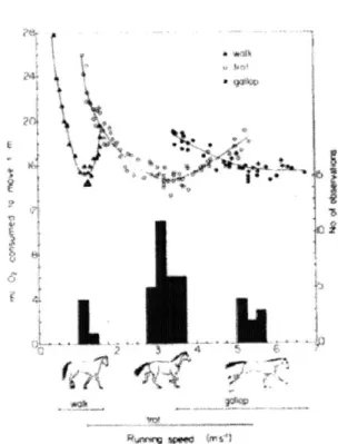
2.2 The major gaits of horses. Metabolic cost of walking, trotting and gal-loping as a function of speed. Hoyt and Taylor [2] suggested metabolic cost as a gait selection criteria. . . . . 28

(12)

2.3 Footfall patterns and timing of three major gaits of horses, walk, trot and gallop, as shown in [3] . . . . 30

2.4 The dynamic characteristics of two different galloping gaits. A dia-gram showing the net impulse vectors of each limb in (a)Horse-like gallop vs. (b)Cheetah-like gallop adapted from [4]. The difference between them is characterized by footfall sequence and the center of mass dynamics as qualitatively shown in (c). Dogs and cheetahs em-ploy both gaits and use rotary gallop in higher speeds. The MIT Cheetah simulation model shows horse-like gallop in a reverse fashion at slow speed (right-bottom plot) and shows cheetah-like gallop at high-speed (right-top corner) [5] . . . . 31 2.5 Cost of Transport of various animals, robots and forms of

transporta-tion [6] . . . .. . . . . 33 2.6 Energy flow diagram of a robotic system. Three major energy loss

modes contribute the total energy expenditure. For the model used in this work the interaction energy was neglected as the massless legs do not create impact losses and no-slip conditions do not accumulate friction losses. . . . . 37

(13)

3.1 The prototype quadruped model used for simulation and optimization.

It is planar with four massless legs and parameters based on the MIT C heetah. . . . . 50 3.2 Individual leg geometry . . . . 53

3.3 Sample of vertical ground reaction forces (GRF) for horses when

walk-ing (A), trottwalk-ing (B) and canterwalk-ing (C) from [7]. The forces of the front limbs are indicated with red broken lines and hind limbs with green broken lines. Beneath the force outputs, the corresponding accelerom-eter traces are shown. Vertical broken lines indicate the timing of foot touchdown (a) and takeoff (b). [7] . . . . 55

3.4 Force profiles are determined by Bezier polynomials. Vertical ground reaction force waypoints are predetermined, optimization simply se-lects scaling for independent feet. Horizontal ground reaction force coefficients are free for optimization. . . . . 57

(14)

4.1 The timing specification and parameterization of each of the gaits studied. This study included a 1-beat gait, pronking, two different 2-beat gaits, trotting, bounding, and a 4-beat gait, galloping. Here the y-axis depicts the specific foot, hind left (HL), hind right (HR), front left (FL) and front right (FR). The pictured gaits each utilize

the same duty ratio, swing time, and period . . . . 67

4.2 G allop . . . . 69

4.3 Trotting . . . . 69

4.4 Bounding . . . . 69

4.5 Pronking . . . . 69

4.6 The optimal motions of each gait studied depicted with fixed period 200 ms, forward speed of 5 m/s, and duty ratio of 1.5. Galloping has a percent overlap of 70%. Legs are not pictured unless they are in contact with the ground. The left legs are depicted with black lines and the right with blue. . . . . 69

4.7 The vertical forces, limit cycles, and knee and hip torques for the bounding optimization for a varying range of duty ratios. The lower the duty ratio the closer to impulsive the force input is. . . . . 70

(15)

4.8 Example of optimal force profile and paired leg motion during stance.

A stance leg is shown in blue, where as the force vector is depicted

in red. Hip torque is also minimized by pointing the force along the virtual leg. Knee torque is minimized by reducing stance time and therefor minimizing the deflection of the knee. . . . . 71

4.9 Cost versus duty ratio for trot and bound. The effects of having either a fixed period or a fixed swing time are shown. In all cases the optimal solution is impulsive. . . . . 72

4.10 Visualization of leg posture changing the effective mechanical advan-tage of a leg [8]. Large ungulates typical utilize larger EMA and a smaller cost of transport than smaller animals. This could be due to the fact that smaller animals may prioritize factors other than ener-getics, such as stability or adaptability due to the relative size of their environm ent . . . . 73

4.11 The effect of changing the percent of stance time overlap for galloping on the cost of joule heating. By increasing the overlap time, the legs are force to take on a more crouched position causing* a higher cost of transport. . . . . 75

(16)

4.12 The effect of interface stiffness is a dynamic foot position due to de-flection. . . . .. . . . 76

4.13 Effect of interface stiffness on optimal duty ratio and CoT for trotting at 3 m/s. Optimal duty ratio increases with a softer interface but the cost of transport is driven down. . . . . 77

4.14 Comparison between effects of interface stiffness on bounding and trot-ting for the same forward velocity. . . . . 78

4.15 Compression during stance time versus force separate by direction. Behavior is non-linear and has directionality associated with the fore/aft direction. . . . . 80

4.16 Cost versus duty ratio for bounding at 3 m/s. Two optimization costs were considered, ct and cet. For each, both the joule-heating cost and

total cost are shown. . . . . 83

4.17 The optimal cost as a function of speed for 4 different gaits, trot, pronk, bound, gallop. The optimal duty ratio was always found to be the lower bound, D = 0.1. . . . . 85 4.18 Cost versus speed for 4 different gaits, trot, pronk, bound, gallop with

(17)

4.19 Comparison of trotting cost with data from the experiments of the MIT Cheetah trotting for fixed swing time and varying stance time. . 87

5.1 Subsystemes that are needed to model the full neuromusculoskeletal system in order to replicate body motions. [9] . . . . 91 5.2 Example activation dynamics of a muscle. The solid line is

excita-tion, u, dotted line is calcium ion concentraexcita-tion, -', dashed line is the

resulting force, fmn. [10] . . .. . . ..... ..... ...92

5.3 A model of a muscle tendon unit (MTU). An active, contractile

el-ement (CE) together with a series elasticity (SE) form the MTU in normal operation [11] . . . . 93

5.4 Visualization of common muscular properties. a) Force-velocity curve for slow muscle. b) velocity curve for a fast muscle. c) Force-length relationship [10] . . . . 94

(18)

(19)

List of Tables

3.1 Parameters and associated values for the prototype model used in this w ork . . . .

4.1 Sample preferredl trotting duty ratios of various animals adapted from [12] . . . .

5.1 Division of energetic cost for human walking as found in [13]. Mechani-cal work only makes up for 31.4% with the rest of the cost encompassed

by different types of muscular heat. . . . . 52

74

(20)

(21)

Chapter 1 Introduction

Quadrupedal animals have the freedom to adopt a wide range of gaits, which allows for great flexibility of motion. The gait, dependent on a particular footfall sequence, is chosen to negotiate challenging terrain, minimize risk of injury [14, 15], or maximize economy of transport [2].

According to the literature, gait selection in nature is triggered by the interplay between physiological causes and dynamical constraints. In the studies of horses, it has been hypothesized that gait selection is governed by energetics in the form of either metabolic cost [2] or peak force production [16]. While the reasons for these preferences are still not fully understood in the animal domain, comparatively less is known about how to effectively manage gait selection in quadrupedal robots.

Understanding optimal running strategies as well as the characteristics of each gait is a pivotal first step for designing controllers for quadruped robots. The intuition gained from studying specifically gait energetics could be useful in future algorithms

(22)

that seek to intelligently and efficiently implement gait selection and transitions. However, there are two main challenges in studying gait characteristics. First, it is difficult to draw useful principles applicable to robotics due to the complexity of lo-comotion. The hybrid nature of terrestrial locomotion dynamics consists of frequent switching between ground contact and take-off. In animals, these complex dynamics are controlled by intricate coordination of neuromuscular systems to achieve desir-able performances. Second, given the differences between mechanical actuators and muscles, it is difficult to predict answers to these questions from animal studies alone. Therefore, this work focuses gait optimization for robotic systems. Motivated by the need for greater understanding of the energetic tradeoffs for a particular robot, the MIT Cheetah, this work seeks to characterize the energetic performance of vari-ous gaits and explore the mechanisms which are responsible for the cost. This study hopes to gain insight into the energetics of running, and seeks to find trends in cost across timing, gait, and environmental parameters for this robotic system. While there have been similar studies for systems with differing sources of actuation, the model utilized here is unique to the Cheetah's design paradigm of proprioceptive force control actuators. As the actuators in this model differ greatly from muscles, a thorough investigation into differences between the two was conducted to better un-derstand which energetic principles are universal optimal across running quadrupeds

of any type and which are confined to the realm of either robotics or animals. While a few other optimization studies have investigated the relationships be-tween gait and energetics, this work represents the first such study applicable to the

(23)

Figure 1.1: Motivation for this study came from the MIT Cheetah. The primary focus was to gain insights into gait energetics which can then be considered for future control algorithms and design

type model of the Cheetah and a minimally complex trajectory optimization

frame-work, this work hopes to gain insights of the governing mechanism in quadrupedal

running for this design paradigm. A purposefully simple model and optimization

allow for general conclusions to be drawn so that they pertain to this class of robots

rather than simply as an artifact of parameter selection. The principles uncovered

in this work help to better understand energetics in actuated robots and presents

considerations to imiprove the energetic efficiency of future designs and control

algo-rithms.

The remainder of this thesis is organized as follows. Chapter 2 describes the

motivation and background for this study including information on types of energetic

cost as well as the results of other similar studies. Chapter 3 details the prototype

(24)

results from case studies which utilized this method to characterize factors that play a role in gait selection. Lastly, Chapter 5 explores the complexity of biological systems and muscles that limit the ability to draw decisive conclusions from animal studies for use in robotic "systems and details the fundamental differences in robot and animal locomotion. Using this model, trends were identified in timing, environmental factors and actuation method. From this information, the optimal gaits for this particular model were identified.

(25)

Chapter 2. Motivation

Animal locomotion is complex, dictated by biological constraints and requirements. Because of the complexity, translating principles to robots can be challenging. One past approach [1] has followed the extraction process shown in Fig. 2.1. The process starts with hypothesizing principles from the comparative study of animals that exhibit targeted behaviors. The principles are then tested by computational models that describe the behaviors and through analyses of simulation data from the models. Based on results from the analyses, control algorithms and mechanism designs may be implemented for experimental validation of the principle.

This process has been successfully applied to a hexapedal running robot, iSprawl

[17], and a wall climbing robot, Stickybot [18]. Also, the MIT Cheetah leg was

developed based on design principles hypothesized through this process [19]. The hypothesis was that tendon-bone co-location architecture can minimize stress on the bone under bending and this principle was previously modeled, analyzed, and

(26)

Rep _{from Comparative study}Hypothesis

Modeling using simple tempplates

Data Analysis & design control Algorithm

Experiments for validation of principles

u ring

Figure 2.1: Schematic of the bio-inspired principle-extraction process [1]. The left diagram represents the difference in constraints of animals and robots, and the coin-mon principles in the intersection between the two domains. The right diagram represents the principle-extraction process composed of four steps allows to abstract out useful principles applicable to robotics research.

validated by experiments

[5].

In the work here, the same bio-inspired engineering philosophy was used to

effec-tively extract principles of optimal running motions and gait selection in quadrupeds

from nature was followed. Inspiration from biology was obtained and used to

for-mulate hypotheses that could be used and tested on a computational model, which

is representative of robotic systems. From this we hope to gain insight not only on

how to control running in quadrupedal robots but also on fundamental differences

between robotic and biological quadrupeds.

2.1 Gait Energetics

(27)

superin-of gait transitions was performed in horses in 1981, which suggested optimization of energy as the driving factor for changing gait [2]. In this study, metabolic cost analysis of the horse indicated that each gait has its own preferred speed, and that energy expenditure increases as the horse deviates from this preferred speed. There-fore, to minimize the cost of energy with speed change, the animal then changes its gait. This trade off is shown in Fig. 2.2. Another study with ponies put forth the idea that the peak force exerted by limb muscles increases within gaits when the speed increases, and drops with gait change, resulting in redistribution and reduction of forces [16]. According to the force hypothesis, the metabolic cost of locomotion is determined primarily by the cost of generating muscular force when the foot is in contact with the ground [20]. The conclusion that leg swing costs are negligible factored heavily into the development of a prevalent theory of locomotor costs [20] and locomotion costs are dominated by the cost of force production.

Granted there are other hypothesis for gait selection; An in vivo experiment from Biewener showed that the strain levels recorded at the trot-gallop transition of the goat were similar to the values reported for the dog and horse [14]. Yet another study, however, showed that the trot-gallop transition occurs at a slower speed when the goat is moving up an incline, which appears inconsistent with this peak force hypothesis [21]. In theory, the change of inclination should not affect the peak force, but the change of inclination does change the transition speed, suggesting a factor at work other than peak force.

Alexander [22] hypothesized that the transition from trot to gallop in quadruped mammals of various sizes, ranging from small rodents to rhinoceros, occur at a Froude

(28)

-*7 VA

L

Figure 2.2: The major gaits of horses. Metabolic cost of walking, trotting and galloping as a function of speed. Hoyt and Taylor [2] suggested metabolic cost as a gait selection criteria.

number between 2 and 3. A recent study in small rodents shows that gait transition speed is neither correlated to energetics nor leg force [23] but also occur at a consistent Froude number of 2.7 to 2.8. This possibly implies that gait selection is also driven

by the body dynamic characteristics.

Other studies used mathematical models that have not been replicated in the natural world. Using a mathematical model, Schoner [24] proposed an interesting hy-pothesis for a stability-driven gait-transition criterion. He hypothesized that animals change their gaits when their intrinsic body dynamics reach the stability boundary.

(29)

Other mathematical models [25] [26] [27] were proposed to describe modulation of the footfall sequence but again without a connection to dynamics of the robot body, making it difficult for roboticist to extract practical principles.

With energetic cost in mind as the deciding factor for switching between gaits, a measure of energetics could first be used to study optimality of motions within a gait. Even within a gait, timing of footfall patterns and body motions could differ. To identify the preferences of these gait details, the computation model will be optimized for energetics to address the following questions:

* Given a specific gait, what are the optimal footfall timings and body motions associated with that gait?

* How is this optimal footfall timings affected by the environment?

These questions are respectively addressed in Chapter 4.1 and Chapter 4.2.

2.1.1 Diversity of Gaits

Most terrestrial mammals are quadrupeds and employ various gait patterns, which each use a different footfall sequence. The diverse set of gaits enables flexibility to traverse different terrains at different speeds while maintaining efficiency and ro-bustness. Amongst the many combinatorial footfall choices, however, each species seems to possess a set of preferred gaits. Horses traditionally prefer walking, trot-ting, cantering and galloping, and select between these, presumably to minimize the metabolic cost of locomotion [2]. Some species of horses, however, tend to pace or

(30)

Walk

LF

Trot

LF-Gallop

Figure 2.3: Footfall patterns and timing of three major gaits of horses, walk, trot and gallop, as shown in [3]

tdlt instead of trot. Outside of the horse family, rodents may bound, gazelles may pronk, and the nuanced timings of gait vary yet further across species.

Even within the gallop, often considered to be the fastest and most asymmetrical gait, there exist two distinctive types, a cheetah-like gallop and a horse-like gallop. These are distinctively different not only in footfall sequence but also in body dy-namics [41: in a horse-like gallop, which has one flight phase per cycle, the height of the center of mass fluctuates once per cycle; in a cheetah-like gallop, which has two flight phases, the height of the center of mass fluctuates twice per cycle. More importantly, the net impulse directions from each footfall are very different from horse to cheetah as shown in Fig. 2.4.

(31)

Pitch-height plot

HL CE (deg)

S heIght anglit (9)

Oheetah-Vike ga flop MIT i cea model

(a) (b) (c) (d)

Figure 2.4: The dynamic characteristics of two different galloping gaits. A diagram showing the net impulse vectors of each limb in (a)Horse-like gallop vs. (b)Cheetah-like gallop adapted from

[4].

The difference between them is characterized by footfall sequence and the center of mass dynamics as qualitatively shown in (c). Dogs and cheetahs employ both gaits and use rotary gallop in higher speeds. The MIT Cheetah

simulation model shows horse-like gallop in a reverse fashion at slow speed (right-bottom plot) and shows cheetah-like gallop at high-speed (right-top corner) [5] sults in the recent development of Bigdog and LS3 from Boston Dyanmics [28],

MIT Cheetah [5], StarlETH [29], and HyQ [30]. These robots was developed

un-der many fundamentally different design paradigms. BigDog, LS3 and HyQ both employ hydraulic actuation which provides the capacity for high-power movements while retaining the precision to perform careful locomotion across sparsely available footholds [31]. StarlETH employs DC motors with series elastic actuators (SEAs), has shown the ability to use multiple gaits to traverse piles of loose lumber [32, 33], and can trot up to 0.7 rn/s. The MIT Cheetah robots [34, 35] are based on pro-prioceptive force control DC motor actuators and have demonstrated running with speeds up to 6 nm/s in laboratory experiments. The design principles embodied in these machines

[34]

have enabled their energetic requirements to be the lowest of these paradigms, reaching levels on par with animals.

(32)

Just as different species of horses exhibit different preferred gaits, it is expected that machines within each of these design paradigms might have different gait pref-erences. Between walking, trot walking, and a flying trot, StarlETH demonstrated a lowest cost of transport at its highest speed trotting [36]. Results in 2D simulations of bounding with SEAs by Remy et al. [37], however, suggest that the energetic requirements in SEA robots would increase after a threshold speed. Xi and Remy

[38] later performed gait optimization on a series elastic biped which found walking

and running to be optimal solutions at low and high speeds respectively. This gait preference matched that of a previous study on a prismatic biped [39]. Remy has also investigated gait characteristics for SEA quadrupeds, and found trotting to be optimal at intermediate speeds and galloping and trotting equal at at high speeds

[38]. Unlike the SEA quadruped, the MIT Cheetah displayed a monotonic decrease

in cost of transport with trotting speed up to 6 m/s[34]. Therefore, simulation for a quadruped with proprioceptive force control DC motors is proposed to study the following:

* For the model of interest, an electrically actuated and force con-trolled quadruped, is there an energetically preferred gait?

* How do gait energetics change with speed?

9 Should energetic cost be expected to go up with higher speeds?

(33)

4 -I - 0 M - 4n

buftI-if

.og Body Mass (kg)

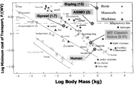
Figure 2.5: Cost of Transport of various animals, robots and forms of transportation

[61

2.2 Cost of Transport

This study attempts to identify energetically efficient gaits; one metric of energetics is the cost of transport (CoT). This quantity, is defined by the energy expenditure E of the gait normalized by its weight, my and distance traveled, Ax.

ZE

Cet = m~

Lo g a s(g

Example values of the cost of transport of various types of animals, robots and forms of transportation can be found in Fig. 2.5. In the biological realm, CoT gen-erally decreases with mass. Also swimmers generally have the lowest CoT, followed

(34)

From a robotics standpoint, there is great diversity in the efficiency of robots, de-pending on their purpose and design strategy. For example, Cornell Ranger, a biped, is able to achieve a low CoT of 0.19 by utilizing passive dynamics [40]. However, this robot is designed specifically for energy efficiency and sacrifices versatility in function [40]. Other legged robots, such as ASIMO with CoT of 2 and BigDog, CoT of 15, are significantly higher than animals with similar masses [41]. It is notable that the CoT for MIT Cheetah 1 was 0.51 [6] and MIT Cheetah 2, 0.45 [34] which rivals similarly sized running animals.

However, there are many ways in which the energy expenditure can be calculated depending on the type of system and the model chosen. Total energy expenditure is perhaps more easily measured, through power or food consumed, than modeled due to the complexities of the system, the environment and the actuators. For example, a complete measure of energy expenditure in the MIT Cheetah would need many realistic components such as LuGre friction model, three-link legs, gearbox model, and encoder noise model, to fully capture the total system energy. Alternatively, biological quadrupeds have equally intricate energy governing components, such as a model of sugar breakdown to make ATP, muscular models of consumption of ATP, and activation delays and noise. These complexities make for challenges in modeling and conclusions that are could be results of specific parameter choices. Rather, different approximations of the energy expended have been developed to simplify the cost of transport in both biological and robotic systems.

(35)

2.2.1 Biological Costs of Transport

From a measure of oxygen consumption, the metabolic rate of energy consumption for a biological system can be estimated. However, the metabolic cost criterion for gait transition was challenged later by the peak force hypothesis, which was formed when researchers observed that when a pony is carrying a load, gait change occurs at a slower speed than the metabolic transition speed [15]. This observation puts forth the idea that the peak force exerted by limb muscles increases within gaits when the speed increases, and drops with gait change, resulting in redistribution and reduction of forces. However, Kram and Taylor found that these hypothesis to be related since the metabolic cost, Emet, can be approximated from factors that decide the ground reaction forces, body weight, mg and ground contact time, t. as [16]

Emet C _(2.1)

mg te

Where c is a cost coefficient unique to a particular animal and computed from data collected from the particular subject. This confirms that the cost of running in animals is primarily due to supporting the animal's weight and the time course of force generation [16].

To model of cost of force generation, the source of actuation must be considered. In the biological realm, the actuation is muscles. Estimating the cost of a muscle can be complicated. For each muscle there are costs caused by the work done by the muscle as well as several muscle specific losses, including activation, mainte-nance, shortening, and basal heats. The muscular losses were found to be nontrivial

(36)

amounts, 68.5% of the total cost for a simulation of a normal human walking [13] making mechanical work an incomplete description of the cost. The activation heat, about 15% of the cost of human walking, is a exponential function of the stimula-tion frequency and is effected by the muscle specific activastimula-tion heat rate and the muscle mass [42]. The maintenance heat, 23%, is related tension in the muscle as well as the activation level [42]. The shortening heat, 8% is extra heat produced as a consequence of the shortening of the muscle and lastly, the basal heat, 22% is the heat dissipated in the parallel elastic structures [43]. These losses depend heav-ily on muscle specific properties and geometries which can make the calculation of muscular costs highly non-generalizable. Since no one specific cost dominates the total energetic expenditure, it is hard to create a low complexity model that truly represents the system.

Also identifying these parameters can be a significant challenge. To estimate the structure of the musculoskeletal system such as moment arms, muscle-fiber and tendon rest lengths, muscle cross-sectional areas, and muscle pennation angles are found using techniques such as computed tomography and magnetic resonance imag-ing [9]. Runnimag-ing performance has been found to be strongly dependent on the values assumed for muscle cross-sectional area, muscle-fiber contraction speed, and the rise and relaxation times for muscle activation [9, 44] so to study the task in great detail, good parameter estimates will be needed on a muscle-by-muscle basis [9]. Therefore making a full and complete muscular model is extraordinarily complex and highly parameterized.

(37)

System Energy Flow Principles Implementation

Ej Eer

wor wok DfflPSeren

Ef I

(Wp-s) MeW Actuated Spne

Figure 2.6: Energy flow diagran of a robotic system. Three major energy loss modes contribute the total energy expenditure. For the model used in this work the interaction energy was neglected as the massless legs do not create impact losses and no-slip conditions do not accumulate friction losses.

2.2.2 Robotic Costs of Transport

In a robotic system, there are multiple energy costs that contribute to the total

system energy expenditure, E. A general breakdown of the energetic costs of a

robotic system is shown in Fig. 2.6 along with design principles to minimize these

losses for systems with proprioceptive force control actuators. Previous studies have

shown that the energetic expenditure in this design paradigm is dominated by the

total joule-heating losses Ej in the motor windings [6]. As the joule heating is related

to torque production, this agrees with the dominance of the cost of force production

seen in the biological realm [16]. Joule heating losses occur in each motor at a rate

of iR, where 1', is the motor armature current and R its terminal resistance.

(38)

Ef in the mechanical domain, as well as any loses that come from the interactions

E with the environment, the dominant one for running being impact losses.

E = E3 + Ef + E2 (2.2)

By counting the energetic loses from the system, the work that occurs inside the

system does not need to be computed in order to have an accurate measure of the total energetic expenditure. However, as calculating the ifnteraction losses may be complicated, many researchers use positive mechanical work to physically account for impact losses as well as regenerative inefficiencies in negative work regimes. This simplified cost, is the mechanical cost of transport, MCoT. Many researchers use this metric, for instance Remy's work on series elastic bipeds and quadrupeds were motivated by this cost [45, 38]. However, as results from MIT Cheetah I indicated that approximately 76% of the total cost of transport came from joule heating, the MCoT may not be a sufficiently encompassing metric to asses robots using proprio-ceptive force control. As a result, investigations into trends in joule heating across gaits will be important to the work herein.

Some of the questions addressed in Chapter. 4.3 are

" How do optimal motions change when optimized for total versus mechanical cost of transport?

(39)

* How does simulation CoT compare to MIT Cheetah CoT and bio-logical Cheetah CoT?

2.3 Muscles vs. Motors

A primary challenge when comparing biological quadrupeds to robotic ones, lies in

the difference between muscles and motors. These differences limit the validity of purely biomimetic design and introduces the need for development and optimization of robotic models. Because of the vast number of differing actuator characteristics, what is optimal for a muscle actuated system may be suboptimal for a motor actuated system.

One key characteristic of an actuator is its force-velocity relationship. Many ac-tuators, including motors, exhibit a linear force-velocity relationship. However when considering muscles as actuators, Hill demonstrated that the force-velocity relation-ship is nonlinear [46]. In particular, for muscles undergoing concentric contractions (where the muscle shortens against an external load), the force velocity curve is de-scribed by a hyperbolic equation. For muscles there is also a nonlinear force length relationship.

There are suggestions as to the effect of the nonlinear force relationships. One theoretical model predicts increased stability and robustness to noise [47]. The ad-dition of muscle-like force velocity nonlinearities in fish locomotion reduces the cost of transport by a factor of 6 [48]. Experiments on nascent myoblasts suggest that hyperbolic force generation allows individual cells to sense the stiffness of their

(40)

envi-ronment [49]. However, these claimed advantages cannot be comparatively tested in experiment, because muscle's nonlinear force-generating properties cannot be altered or controlled in-vivo.

Seyfarth studied a jumping leg with both pure springs and muscle tendon units

[50]. In his studies he found that the addition of a muscle tendon unit shifted the

timing of maximum force from mid stance to occur almost simultaneously as maxi-mum shortening velocity due to the steep increase of the force-velocity relationship. He also found that the elastic behavior of the system is a result of fast loading of the muscle-tendon complex and is largely limited by muscle properties, namely the force-length and force-velocity curve.

However, in terms of gait energetics in quadrupeds, there is much left unexplored. Some of the questions addressed in Ch. 5 are

* How do optimal motions change when actuated by muscle or motor? * How do the nonlinear force relationships of muscle constrain/aid the

optimal solution?

* How does cost shift due to actuator choice?

Despite extensive studies of optimal gaits in quadrupedal animals, it remains chal-lenging to pinpoint the exact criteria controlling gait selection, due to its complex nature. In addition to the sometimes conflicting kinematic, energetic, and mechanical perspectives discussed above, studies have also investigated the role of muscle

(41)

phys-gradually, across a wide range of speeds and associated with discontinuous changes in energy use. Given such a wide range of variables, it is not surprising that we lack integrative models representing the complex hybrid dynamics of quadrupedal animals [53]. Moreover it is challenging, given our current limited understanding of why, how, and when gait selection occur, to extract principles applicable to robotics. Exploring this biological complexity serves as our motivation to utilize engineering tools to investigate the intrinsic dynamics of each gait.

(42)

Chapter 3 Framework for Studying Gait

Energetics of Electrically Actuated

Quadrupedal Robots

To answer the questions proposed above, a simple model of an electrically actu-ated quadruped was developed to simulate and optimize. For this work, a minimally complex trajectory optimization framework and model of the MIT Cheetah were pur-posefully chosen to promote the generality of the findings to this class of quadrupedal actuation. This is the first such study of a model related to the design paradigm of proprioceptive force control and the framework developed here will help uncover insights relevant for future control algorithms and design choices for this type of quadrupedal robot.

(43)

related to gait energetics. Since the work searches for optimal gaits, this chapter will first detail the principles behind trajectory optimization and then highlight the choices made for optimization formulation in this work. Next, the prototype model will be introduced with specific attention to the formulation of dynamics and param-eterization of state and control for optimization.

3.1 Trajectory Optimization

Trajectory optimization is a powerful framework for planning locally optimal tra-jectories for linear or nonlinear dynamical systems. Given a control system, and an initial condition of the system q(O), trajectory optimization aims to design a finite-time input trajectory, u(t), Vt E [to, tfI, which minimizes some cost function over the resulting input and state trajectories.

The optimization problem is to minimize the cost, J

J= <D[q(to), to, q(tf), tf, T] (3.1)

where q(t) is the state history, to is initial time, tf is the final time and T is a optimization parameter vector.

The state history is constrained to satisfy the given dynamics

(44)

They must also satisfy specific path constraints

Cmin < c[q (t), u(t), t, T] < cm,,,, (3.3)

as well as specified end constraints

bmin b[q(to), to, q(tf), tf, s, T] bax (3.4)

Also the optimal control problem can be formulated with multiple phases, where a unique phase is created when the dynamics or constraints of the problem differ. In the case of a running quadruped a change of phase is marked by the touchdown or takeoff of a foot. Phases can be chained together with imposed phase boundary constraints.

There are a number of popular methods for transcribing the trajectory optimiza-tion problem into a finitely parameterized nonlinear optimizaoptimiza-tion problem. Broadly speaking, these transcriptions fall into three categories: dynamic programming, in-direct methods, and in-direct methods.

In dynamic programming (DP), the goal is to find a solution of the Hamilton-Jacobi-Bellman (HJB) equation, which gives sufficient optimality conditions for an optimal solution. To find a function, satisfying the HJB partial differential equation, the continuous state and control spaces are sampled for each discrete state. The solution is iteratively approached by minimizing the sum of the costs for the next time step and the cost-to-go from the sampling point reached in the next time step

(45)

sequence. This procedure goes back to Bellman's principle of optimality, which proves that the remainder of an optimal trajectory is also optimal. The optimal continuous and discrete control can be calculated directly from the optimal value function. Since the value function depends on the continuous and discrete state, the optimal control is a feedback control, which is valid in the bounds of the sampled state space. A solution found by DP is globally optimal since the HJB equation provides sufficient optimality conditions. Furthermore, DP algorithms are globally convergent in the sampled state space starting from an initialization with zeros and provide a closed-loop feedback control. However, DP is plagued by the "curse of dimensionality" which describes the exponential increase of complexity in the number of continuous states and controls and limits the applicability of DP to problems with few states and continuous dynamics.

In indirect methods, necessary optimality conditions for an optimal solution are formulated and derived, generally utilizing techniques extended from the calculus of variations, and lead to a multi-point boundary value problem. The boundary value problem consists of the differential equations of the state and its dual state, the adjoint, an algebraic equation specifying the optimal control, and boundary conditions. The boundary value problem is then solved numerically, usually by a Newton method, since the problems are generally difficult or impossible to solve analytically. The small domain of convergence and the difficult initialization are two of the main drawbacks of indirect methods.

Direct methods first discretize the initial guess for the continuous state and con-trol trajectory with respect to time. The discretized state and concon-trol values at

(46)

the time nodes are varied by a nonlinear programming (NLP) algorithm such that the cost criterion is minimized. Simultaneously with the minimization, the system dynamics and boundary conditions, which are formulated as constraints, have to be satisfied at. certain points of time. Direct methods have a large domain of con-vergence compared to indirect methods, are not too difficult to initialize and often provide solutions with an acceptable accuracy. Furthermore, direct methods can be adapted flexibly to different classes of optimal control problems without much effort. The disadvantages of direct methods are that solutions are only locally optimal and only open-loop controls can be determined.

In this work, only direct methods were considered because of their relative sim-plicity, as they do not require the derivation of optimality conditions, and because of the tendency for the resulting NLP problems to be be easier to solve computationally than the boundary value problems of indirect methods, especially without any prior

knowledge of the solution. Direct methods are further classified by the manner in which the optimal control problem is discretized into two subcategories, the shooting methods and the direct collocation methods.

3.1.1 Shooting Methods

In shooting methods, the nonlinear optimization searches over a finite parameteriza-tion of the control input u(t), using a forward simulaparameteriza-tion from the initial condiparameteriza-tion,

q(O) to evaluate the cost of every candidate input trajectory. The dynamics and

(47)

prop-the first phase to prop-the final conditional as prop-the final phase.

The simulation works as follows. The equations of motion for a running quadruped constitute a hybrid dynamic system in which phases of continuous motion are in-terrupted by discrete events, namely footfalls. Such problems are typically solved approximately using a numerical integration scheme that propagates the solution forward iteratively through successive points in time by solving an equation related to the dynamics. The initial boundary value problem for the hybrid system is solved

by propagating the continuous dynamics forward until a specified event is detected.

Numerical integration stops, the boundary conditions and dynamics are applied, and numerical integration continues.

The shooting problem is thus to search for the initial conditions of the first phase q(O), static parameters T, and a finite number of parameters describing the continuous control trajectory u(t) that results in the the minimum of the objective function while satisfying the constraints.

3.1.2 Direct Collocation Methods

In direct collocation methods,a nonlinear optimization problem is formulated over parameterizations of the control and state, u(t) and q(t); here no simulation is required and instead the dynamics are imposed as a set of optimization constraints, typically evaluated at a selection of collocation points. Now, the problem is to search not only for the initial conditions q(O), static parameters T, and a finite number of parameters describing the continuous control trajectory u, but also a finite number of parameters describing the continuous state trajectory q.

(48)

Direct collocation methods typically enjoy a considerable numerical advantage over the shooting methods. Shooting methods are plagued by poorly conditioned gradients; for instance, a small change in the input tape at t = 0 will often have a

dramatically larger effect on the cost than a small change near time T. Direct meth-ods can also be initialized with an initial guess for the state trajectory, q(t), which can often be easier to determine than an initial tape for the control, u(t). A reason-able initial tape is generally helpful in avoiding problems with logal minima. The resulting optimization problems are also sparse, allowing efficient (locally optimal) solutions with large-scale sparse solvers, and trivial parallel/distributed evaluation of the cost and constraints.

Software Used

The particular collocation scheme used in the work, a Gaussian quadrature collo-cation method, GPOPS II, is described in detail in [54] but the essential idea is that this method converts the infinite-dimensional, continuous-time problem into a finite-dimensional problem by transcription, where the time histories q(t) and u(t) are approximated by Lagrange interpolating polynomials, which interpolate between collocation points. Polynomials are constructed to approximate the trajectory of the state derivative globally, that is, over the entire interval which exactly satisfy the differential equations at the collocation points. These interpolating polynomials can then be integrated exactly. A key benefit is that this method offers an exponential convergence rate for the approximation of analytic functions [55]. More specifically,

(49)

[54], in Matlab R2014b.

Such problems are solved numerically by any of several nonlinear programming algorithms. In general, these programs utilize gradient information to locate local minima, but there are many different and increasingly effective methods and solvers. In the work here, IPOPT was utilized which is an interior point algorithm and is detailed in [56].

3.1.3 Optimization Caveats

It is important to note that the optimal trajectories found in this thesis are only locally optimal since these problem formulations are not strictly convex. They are also heavily dependent on the initial guess. The solver is also sensitive to the the variable bounds, tolerances, mesh parameter and differentiation methods. While this can make it nearly impossible to exhaustively check for definitive results, it can still be a powerful tool for identifying trends in a local space.

Several tactics were used to ensure valid results despite the complexities and limitations of these optimization strategies. In order to encourage feasibility of the problem formulation the optimization was warm started, using feasible solutions from previous trials to initialize the following trial when sweeping over a range of parameter values. If the optimization failed to find a feasible solution, a reseeding strategy was used to alter the original local search space. These reseeding strategies involved warm starting with other feasible previous identified solution or perturbing the initial tape or the static parameters. Alternatively if the feasible result appeared

(50)

b (~y

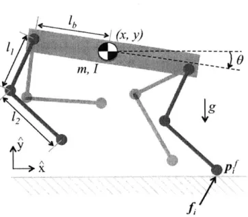
Figure 3.1: The prototype quadruped model used for simulation and optimization. It is planar with four massless legs and parameters based on the MIT Cheetah.

to be on outlier compared to the trend of surround points, reseeding was also applied in order to ensure smooth curves out of these methods.

3.2 Template Model

A simple quadruped model was chosen, shown in Fig. 3.1, that embodies the design

principles of the MIT Cheetah. This planar model includes four massless legs that are used to deliver ground reaction forces to a rigid torso. The simplicity of this model was chosen to promote the generality of the findings to a broad class of quadruped robots with relatively backdrivable actuators. In comparison to a high-fidelity model, this reduction in complexity benefits the gait optimization detailed in Section 3.1 by

19 MY O 2 A A X

(51)

realistic representation of the real MIT Cheetah design. For instance, the MIT Chee-tah's legs account for only approximately 10% of the total system mass. However,

by neglecting the leg mass and inertia, we neglect their effects on impact losses and

the costs of leg motion that require positive mechanical work as shown in Fig. 2.6. Previous experiments with the MIT Cheetah I [34] show that these factors make up only 20% of the cost of transport. Thus, this work focuses on trends in joule-heating losses which dominate the CoT in these machines. This decision will be validated with an investigation into cost in Ch. 4.3.

3.2.1 Model Dynamics

The quadruped model used in this work is shown in Fig. 3.1. Model parameters were based roughly off of the MIT Cheetah whose values can be found in Table 3.1. Since the legs of the model used are massless, their positions while in the air do not matter in determining the system dynamics. Thus, instead of including the legs as states, their dynamics are fully described with a single foot stance location,

P E R2 with the subscript i E {1,..., 4} denoting the specific foot. Considering

no-slip conditions, the stance location is simply a constant, determined by a horizontal touchdown position, xD E R, and the ground height, yg E R.

In this manner, the robot can be simplified to a 3 degree of freedom system with generalized coordinates, q = XY, ,] , as shown in Fig. 3.1. The dynamics for this

(52)

symbol parameter value units

m body mass 32 kg

I body inertia 2.9 kg-m'

it body half length 0.4 m

'1 upper leg length 0.25 m

2 lower leg length 0.25 m

Table 3.1: Parameters work

and associated values for the prototype model used in this

system can be given as follows.

4 mxz=

_{Z f[}

4 m D= -m g + f i

I=

p-

x

fi

*=1J ) (3.5) (3.6) (3.7)

The horizontal and vertical ground reaction forces (GRFs) for each foot are

col-lected in the vector

f,

=

[fH,

fi]T E R2. In order to transform these forces into

equivalent joule-heating losses, a Jacobian is needed for each individual leg. Given

the kinematic leg parameters 11, 12 shown in Fig. 3.1 and the relative foot position

rel _{= Ph - P4}

pA =i I)

(3.8)

(53)

(xh, yh)

l 3

\p relil

(x1, 0)

Figure 3.2: Individual leg geometry

Then inverse kinematics can be computed to find the hip and knee angles of each

-T

leg <h

LI4liP,

Okn . Looking at an individual leg in Fig. 3.2 and using the law of

cosines, this is calculated as

(1 _ 2 + _prel

hip / - tan- (3.10)

okn _hip

-sin1 (Xh - (3.11)

where 11 and l2 are given leg segment lengths. A Jacobian for each leg, Ji (p el) E R2x2, can then be computed as

&prel

Ji = ap . (3.12)

(54)

Joint torques for each leg ri = ip, are then computed from the relative foot

position and GRF as:

ri = Ji _{(Prel)T f.} Where (11 + l2) cos(01'' + #f") - li cos(4hip) -(li + 12) cos(75" + ") (l1 + 12) sin(o4hi + #f") + 1, sin(1NP) (l + 12) sin(#5'Z I$")

We note that since the legs are assumed massless, this transformation is exact not just in static conditions, but also during dynamic motion.

3.2.2 Ground Reaction Forces

The MIT Cheetah is actuated by proprioceptive force control DC motors, meaning than its controller attempts to produce specified forces without explicit force sensor feedback at the foot. In particular the scheme attempts to produce biologically similar ground reaction forces, as seen in Fig. 3.3. When running, these GRF profiles are single hump peaks unlike walking which displays double humped GRFs.

Force Profile Reduction for Optimization

(55)

4jA B b aB a b C 1 B / 6 a b 3 % I (00 10M 1400 ISM 2200 2600 800 1000 1200 1400 130 1350 1400 1450 1500 ime (ms)

Figure 3.3: Sample of vertical ground reaction forces (GRF) for horses when walking

(A), trotting (B) and cantering (C) from [7]. The forces of the front limbs are

indicated with red broken lines and hind limbs with green broken lines. Beneath the force outputs, the corresponding accelerometer traces are shown. Vertical broken lines indicate the timing of foot touchdown (a) and takeoff (b). [7]

between its touch down, t? and liftoff, tf, times. When airborne, no force may be

applied. For optimization, low-order Bezier polynomials are considered to enforce

smoothness of these control inputs and mimic force profiles seen in animals. The parameterization of these polynomials is described as follows.

Specifically, forces are formed as,

Sb j,, , if tq < t < t {Zbnx(I )0 i3 if tZtt (.3

fr

(t) = j:o (3.13) 0 else bj,n. Oy. if tq < t < tf ff () = i (3.14) 0 else

Where bj,(-) : [0, 1] -+ R is the j-th Bernstein polynomial or order n, and each

cj

(56)

described in Fig. 3.4. The shape of the vertical force was fixed through a low-order polynomial with constant coefficients aj to produce a single hump profile. A scaling of this shape was then optimized with coefficient, a& E R, for each foot as in [6]

providing /3j = [/ii, ... , i3,]j as

#= i 10 a, ... _{a,_- 0}

-Specifically, the vertical force profile was chosen to use two distinct 3rd B6zier

polynomials, one for the first half of stance and one for the second. The coefficients were selected for smoothness, symmetry and easy scaling.

ai 0.0 0.8 1.0 1.0] if to < t < 0.5(tf - t?) + to

ai [1.0 1.0 0.8 0.0] if 0.5(t- Z

) +It9t t

The horizontal force profile was selected as 4th order, n, = 4 with its non-zero coefficients as optimization parameters.

i =

[0

Oii A2 A3 0] (3.15)

Thus, the forces during a stride for leg i are described in total through four parameters for optimization [ai, Oil, /3i2,

/

3i31.

(57)

-- Hind --Fr ont 1 2

0

0.02 0.04 0.06 0.08 0.1 0.12 0.14 0.16 0.18 0.2 Time (s) -Hind --- Front - i23 fil P21 P 22 Pi*12I 0 0.02 0.04 0.06 0.08 0.1 0 Time (s) .12 0.14 0.16 0.18 0.2

Figure 3.4: Force profiles are determined by Bezier polynomials. Vertical ground reaction force waypoints are predetermined, optimization simply selects scaling for independent feet. Horizontal ground reaction force coefficients are free for optimiza-tion. 500 400 C 300 200 100 0 -4 L 150 100 50 0 -50 -100

(58)

3.3 Optimization Formulation

This study attempts to identify energetically efficient gaits, and thus can be expressed as trajectory optimization to minimize the total energetic cost of transport (CoT). This quantity, c et E R is defined by the energy expenditure E of the gait normalized

by its weight and distance traveled.

E

Cet =

mgAx

To shape these costs, each foot has a set of optimization parameters Xi E R5

which includes,

" horizontal force Bezier coefficients, Al, A2, /3-3

" vertical force scaling coefficient, ao

" touchdown position, xTD

However, some symmetry and equality between foot parameters is enforced based on the selected gait. For instance, in bounding the left and right feet of the front/hind pairs operate together, reducing the problem to effectively 2 independent feet. With

M as number of independent feet, the optimization parameter vector is denoted as X E R5 . The state trajectory q(t) is optimized over one period and is enforced to be consistent with these parameters X.

Characterization of gait energetics for electrically actuated quadrupeds

@Massachusetts

Signature redacted

MAR

0

2

016

Signature redacted

Contents

List of Figures

List of Tables

Chapter 1

Introduction

Chapter 2.

Motivation

[5].

2.1

Gait Energetics

L

2.1.1

Diversity of Gaits

[4].

[34]

[61

2.2

Cost of Transport

2.2.1

Biological Costs of Transport

2.2.2

Robotic Costs of Transport

2.3

Muscles vs. Motors

Chapter 3

Framework for Studying Gait

Energetics of Electrically Actuated

Quadrupedal Robots

3.1

Trajectory Optimization

3.1.1

Shooting Methods

3.1.2

Direct Collocation Methods

3.1.3

Optimization Caveats

3.2

Template Model

3.2.1

Model Dynamics

Z f[

I=

p-

x

fi

f,

[fH,

LI4liP,

3.2.2

Ground Reaction Forces

fr

cj

[0

/

0

3.3

Optimization Formulation

_{Z f[}