HAL Id: hal-00317442
https://hal.archives-ouvertes.fr/hal-00317442
Submitted on 1 Jan 2002
HAL is a multi-disciplinary open access
archive for the deposit and dissemination of
sci-entific research documents, whether they are
pub-lished or not. The documents may come from
teaching and research institutions in France or
abroad, or from public or private research centers.
L’archive ouverte pluridisciplinaire HAL, est
destinée au dépôt et à la diffusion de documents
scientifiques de niveau recherche, publiés ou non,
émanant des établissements d’enseignement et de
recherche français ou étrangers, des laboratoires
publics ou privés.
Theoretical simulation of O+ and H+ densities in the
Indian low latitude F-region and comparison with
observations
P. K. Bhuyan, P. K. Kakoty, S. B. Singh
To cite this version:
P. K. Bhuyan, P. K. Kakoty, S. B. Singh. Theoretical simulation of O+ and H+ densities in the Indian
low latitude F-region and comparison with observations. Annales Geophysicae, European Geosciences
Union, 2002, 20 (12), pp.1959-1966. �hal-00317442�
Annales Geophysicae (2002) 20: 1959–1966 c European Geosciences Union 2002
Annales
Geophysicae
Theoretical simulation of O
+
and H
+
densities in the Indian low
latitude F-region and comparison with observations
P. K. Bhuyan1, P. K. Kakoty1, 2, and S. B. Singh1
1Department of Physics, Dibrugarh University, Dibrugarh 786004, India 2Department of Physics, North Lakhimpur College 787031, India
Received: 11 June 2001 – Revised: 6 June 2002 – Accepted: 20 June 2002
Abstract. The O+and H+ion density distributions in the
In-dian low latitude F-region, within ±15◦magnetic latitudes,
are simulated using a time dependent model developed on the basis of solution of the plasma continuity equation. The simulated ion densities for solar minimum June and Decem-ber solstices are then compared with ionosonde observations from the period 1959–1979 and measurements made by the Indian SROSS C2 satellite during 1995–1996 at an altitude of ∼500 km. The simulated O+density has a minimum around pre-sunrise hours and a maximum during noontime. H+ den-sity is higher at nighttime and lower during the day. The simulations reproduced the well-known equatorial ionization anomaly (EIA) observed in electron density at the peak of the F2-region in the Indian low latitude sector during solar minimum. In situ measurement of O+density by the SROSS
C2, however, showed a single peak of ionization around the equator.
Key words. Ionosphere (equatorial ionosphere; modeling and forecasting)
1 Introduction
The distribution of plasma in the ionospheric F-region de-pends on the three processes of production, loss and trans-port. At equatorial and low latitudes, the F-region is charac-terized by a depression in ionization densities at the magnetic equator and two maxima on either side of the equator. Be-sides this well-known phenomenon of equatorial ionization anomaly (EIA), the equatorial ionosphere is known to ex-hibit some unique features such as the equatorial electrojet, the spread-F, etc. The horizontal orientation of the geomag-netic field lines at the equator and the shift between the ge-ographic and geomagnetic equator are known to be the main reasons for observation of these features and their longitu-dinal variation. Martyn (1947) put forward the explanation that the E-region eastward electric field at the equator causes
Correspondence to: P. K. Bhuyan ([email protected])
the F-region plasma to drift upward during the daytime. As the plasma is lifted to greater heights, it diffuses downward along geomagnetic field lines under the twin action of grav-ity and pressure gradients (Hanson and Moffett, 1966). A plasma fountain thus forms which moves ionization from the equator to the two anomaly crests. After sunset, the elec-tric field reverses in direction and the F-region plasma drifts downward. The fountain reverses and the crests disappear. The location of the two anomaly peaks shifts towards higher latitudes with increase in E × B drift velocity. Asymmetric neutral winds about the equator produce a north south asym-metry in the EIA. The latitudinal extent of the crests also varies with solar and magnetic activity. The fountain rises to several hundred kilometers at the equator and the crests be-come weaker with increase in altitudes. At higher altitudes, a single crest of ionization forms over the equator (Su et al., 1995; Balan and Bailey, 1995). Rishbeth (1977), Rajaram (1977), Moffett (1979), Anderson (1981) and Stening (1992) have reviewed the characteristics of the equatorial ionization anomaly and associated physical processes.
Many attempts have been made in the past to theoretically investigate the dynamics of the low latitude ionosphere. Em-pirical models such as that of Bradley and Dudeney (1973) and the International Reference Ionosphere (Bilitza, 1990) are useful in describing the “climatology” of the ionospheric regions and their average behavior. Rush (1986) discussed the various kinds of empirical models and how they can be used to make prediction of radio propagation conditions. But empirical models fail to provide any insight into the iono-spheric processes which govern the day-to-day, solar, mag-netic and seasonal variability of ionospheric parameters. On the other hand, theoretical models being sensitive to choice of input parameters can be used to investigate the effect of changes in solar or particle production rates, neutral winds or E × B drifts or variations in neutral atmospheric con-stituents. Bramley and Peart (1965), Hanson and Moffett (1966) and Bramley and Young (1968) solved the time inde-pendent plasma continuity equation to study the formation of the EIA. Baxter and Kendall (1968) qualitatively explained
1960 P. K. Bhuyan et al.: Theoretical simulation of O+and H+densities the daily variation of the EIA by solving a time dependent
continuity equation. Sterling et al. (1969) studied the effect of neutral winds in maintaining the night-time low latitude F2-region plasma densities and that of E×B drift velocity on the position of the anomaly peaks. Anderson (1973 a, b) and Chan and Walker (1984 a, b) derived theoretical models to in-vestigate the EIA structure in the American and East Pacific sectors. Bailey and Balan (1996) and Bailey et al. (1997) described the Sheffield University Plasmasphere Ionosphere model (SUPIM) in which time dependent equations of conti-nuity, momentum and energy balance are solved along closed field lines to calculate the electron and ion densities and tem-peratures at middle and low latitudes. It has been shown that the equatorial plasma fountain is confined to a particular re-gion in altitude and latitude and outside this rere-gion plasma flows towards the equator from both hemispheres. The up-ward flow of plasma outside the fountain region can cause convergence of plasma above the F-region peak close to the equator leading to the formation of an additional layer F3. Using the SUPIM, Balan et al. (1997a) have found that the north-south asymmetries of the equatorial plasma fountain and equatorial anomaly are more dependent upon the dis-placement of the geomagnetic equator from the geographic equator. Watanabe et al. (1995a) had used a time dependent three-dimensional simulation procedure to study the varia-tion of electron and ion temperature and density within ±30◦ and 200 km to 1000 km altitude region. Their results show that the structure of the equatorial ionospheric F-region is strongly affected by the plasma drift which is induced by the ionospheric electric field, neutral wind, exospheric tempera-ture and intensity of solar flux variations. Balan et al. (1997b) theoretically described a plasma temperature anomaly in the equatorial topside ionosphere. Bhuyan and Kakoty (2001a, b) have recently simulated the ion density distribution in the topside F-region of the Indian low latitude ionosphere for so-lar minimum equinoctial conditions and compared the results with the density measurements made by the Indian SROSS C2 satellite.
In this study, the results of the simulation of O+ and H+ density distribution in the low latitude F-region during low solar activity June and December solstices are presented. The model results are then compared with foF2 measurements from 1959–1979 and ion density measured by the SROSS C2 during 1995–1996.
2 Simulation
The ion density in the equatorial ionosphere is simulated by solving the ion continuity equation
∂N
∂t =P − L − ∇.(N V ) (1)
by following the procedure adopted by Bhuyan and Kakoty (2001 a, b). In Eq. (1), N is the ion (electron) density, P and L are the ion production and ion loss rates, respectively and V is the ion transport velocity. Equation (1) is solved
-40 -30 -20 -10 0 10 20 30 40 50 60 0 4 8 12 16 20 0 deg. 10 deg. -10 deg. -30 -20 -10 0 10 20 0 4 8 12 16 20 0 deg. 10 deg. -10 deg. Uθ , m.sec -1 June solstice December solstice LOCAL TIME, hrs
Fig. 1. Diurnal variation of neutral wind velocity for December
(top) and June solstice (bottom) at three fixed geomagnetic lati-tudes.
numerically for O+and H+ions along closed magnetic field lines around the equator under the influence of E × B drift and neutral winds. The production of O+ is assumed to be caused entirely by x.u.v. (extreme ultraviolett) solar radiation (Anderson, 1973a) while H+production is due to the reso-nant charge exchange reaction with oxygen (Stubbe, 1970). The chemical reaction rates are as given by Raitt et al. (1975) whereas the rate coefficients for loss of O+following charge
exchange reactions with O2and N2are taken from St
Mau-rice and Torr (1978) and Bailey and Sellek (1990) respec-tively.
The concentrations of the atmospheric constituents O, O2,
N2 and H are calculated from the MSIS-86 thermospheric
model (Hedin, 1987) as a function of altitude, latitude and local time. The neutral gas temperature (Tn), ion temperature
(Ti) and electron temperature (Te) are chosen from the IRI-90
model (Bilitza, 1990).
The horizontal meridional component Uθ is given by
(Chauhan and Gurm, 1980)
P. K. Bhuyan et al.: Theoretical simulation of O+and H+densities 1961 2 -15 -10 -5 0 5 10 15 0 4 8 12 16 20 -8 -6 -4 -2 0 2 4 6 8 10 0 4 8 12 16 20 Veq , m.sec -1 June solstice December solstice LOCAL TIME, hrs
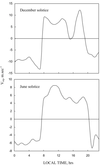
Fig. 2. Local time variation of equatorial vertical E × B drift
veloc-ity in December (top) and June solstice (bottom) over Trivandrum.
where φ is the local time (in hour angle), φois the local time
when the daytime pole-ward neutral wind reaches a maxi-mum, δois the declination of the sun. It is assumed that, Uθ
is independent of altitude. The parameter τ is used to pro-duce a diurnal asymmetry in the wind field i.e. the velocity amplitude is larger at night than in the daytime (Fig. 1). This asymmetry is introduced to allow for the fact that the retard-ing effects of ion drag on the neutral winds are greater durretard-ing the daytime than that at night.
The E × B plasma drift velocity has been measured routinely by the incoherent scatter technique at Jicamarca (70◦W) and reported extensively in literature (Woodman, 1970: Fejer, 1981). The HF Doppler radar developed at the University of Kerala (Balan et al., 1992) provided sys-tematic measurement of F-region plasma drifts at the equa-torial station Trivandrum (77◦E, .3◦S dip). The drifts have day-to-day, seasonal and solar cycle variation. However, the drift velocities measured by the HF Doppler radar technique are apparent, as the delay caused by the ionization along the traversed path has not been taken into account.
Jayachan-dran et al. (1987) noted that the decay in ionization in the evening hours is unlikely to alter the basic pattern of veloc-ity variation in any significant way. Balan et al. (1992) have shown that the uncertainty due to layer decay in the 15:00– 02:00 LST period corresponds to about 0.5 m s−1under nor-mal conditions and 2–3 m s−1under spread-F conditions. In our present calculation, the equatorial value of drift velocity, Veq given by Namboothiri et al. (1989) is adopted as shown in Fig. 2 without ionospheric correction. As the present sim-ulations are carried out for the quiet ionosphere, the above mentioned error, less than 5% of the minimum drift velocity at solar minimum, is unlikely to affect the calculated density.
3 SROSS C2 RPA measurements
The Indian satellite SROSS C2 was launched on 4 May 1994, into an orbit of 46◦ inclination and 930 km apogee with
430 km perigee. In July 1994, the orbit of the satellite was trimmed to 630 km by 430 km. Two Retarding Potential An-alyzer (RPA) sensors were placed on board the satellite for in situ measurement of ionospheric electron and ion densities, temperatures and other related parameters of plasma. The “potential probe” is used to estimate the satellite potential with respect to ionospheric plasma. Both the electron and ion RPA sensors, which consist of four grids and a collector electrode, are mechanically identical but provided with dif-ferent grid voltages suitable for collection of ions and elec-trons. The charged particles, whose energies are greater than the applied voltage on the retarding grid, pass through var-ious grids and finally reach the collector electrode to cause the sensor current. This current is measured by a sensitive linear electrometer. Thus, by changing the bias voltage on the retarding grid, flux of different energy ranges can be mea-sured. The collector current (I ) versus retarding bias voltage (V ) generates characteristic curves separately for electrons and ions which are used to derive total ion density (Ni), ion
composition (O+, O+2, NO+, H+, He+), ion temperature (Ti)
and electron temperature (Te).
In this analysis, we use measured values of ion composi-tion (O+and H+) derived from the RPA data collected during the period August 1995–July 1996. The 10.7 cm solar flux, corresponding to the period of observation, varied between 69.6 and 77.5. The average height of the satellite passes was ∼500 km, which covered the geographic latitude belt of 31◦S–34◦N and longitude belt of 40◦E–100◦E.
4 Results
Equation (1) is solved along centered dipole magnetic field lines, from a base altitude of 120 km in the northern hemi-sphere to the same altitude in the southern hemihemi-sphere. The plasma associated with a particular field line can move to a different magnetic field line at different altitude under the influence of the E × B drifts during the course of the sim-ulation. During the solar minimum period under study, the plasma at the base of the ionosphere can reach a height of
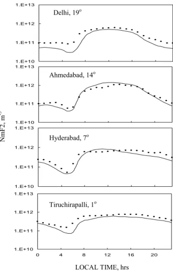
1962 P. K. Bhuyan et al.: Theoretical simulation of O+and H+densities 3 1.E+10 1.E+11 1.E+12 1.E+13 0 4 8 12 16 20 1.E+10 1.E+11 1.E+12 1.E+13 0 4 8 12 16 20 1.E+10 1.E+11 1.E+12 1.E+13 0 4 8 12 16 20 1.E+10 1.E+11 1.E+12 1.E+13 0 4 8 12 16 20 Delhi, 19o Ahmedabad, 14o Hyderabad, 7o Tiruchirapalli, 1o LOCAL TIME, hrs N mF2, m -3
Fig. 3. Measured and simulated NmF2 (shown by dots and solid
line, respectively) for selected locations along 75◦E meridian. The dots are averages of all data for the December solstice solar mini-mum conditions during 1959–1979.
700 km within a period of 24 h of simulation. In order to provide reasonable 24 h coverage of the model values within a specified altitude and latitude region, the model equation needs to be solved along many tubes of plasma (Bailey and Balan, 1996). In the present study, 11 field lines have been considered with apex altitude between 200 km and 1600 km. This limits the altitude resolution of the calculations to a few hundred kilometers above the F-region peak. To overcome the problem of the gap created by the drifting plasma at lower altitudes, more points have to be added to the bottom of the flux tube (Millward et al., 1996) or have enough points in the flux. Another way of overcoming this problem is to solve the equations along the lowermost flux tube at different lo-cal times (Bailey and Balan, 1996). In the present study, the simulations have been carried out for different local times starting at 06:00 LT with a time increment of 15 min for the next 48 h for the lowermost field line. For other field lines, the simulations are carried out for two diurnal cycles starting at 06:00 LT with equal time increments of 15 min. Thus, a two dimensional grid of points in altitude and latitude is
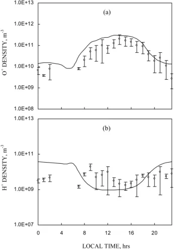
pro-duced for each local time, from which the data at any local time, latitude and height can be recovered taking into con-sideration the drift of plasma at each time interval. It may also be noted that we have considered the vertical drift to be independent of height. In Fig. 3, NmF2, observed at the low solar activity December solstice during the period 1959– 1979 over Tiruchirapalli, Hyderabad, Ahmedabad and Delhi, are shown with the simulated NmF2 at the respective loca-tions. The simulated values of NmF2 are in good agreement with the measured NmF2 at all the locations. The figure indi-cates that the model also generates the observed well-known equatorial ionization anomaly (EIA) with its peak around Ahmedabad and trough at the equator. The electron density is considered to be equal to the sum of the O+ and H+ion densities. In the ionosphere F-region, it is a good approxi-mation (Watanabe et al., 1995a). Figure 4a shows the sim-ulated and observed diurnal variation of O+for the
Decem-ber solstice (NovemDecem-ber, DecemDecem-ber, January and February) at an altitude of 500 km above the geomagnetic equator. The observed density rises in the post-sunrise hours and forms a broad daytime plateau. Diurnal maximum is observed at around 15:00 LT. The afternoon decrease in O+ density is slow and secondary post sunset enhancement is absent. The simulated O+ density fits well with the observed data ex-cept for a few hours in the evening. The theoretical and observed daytime peak values are ∼ 4.8 × 10¹¹m−3 and ∼ 3.4 × 10¹¹m−3, respectively. The diurnal variation of H+density (Fig. 4b) shows a depression during daytime and higher values at night. In the F-region, below 500 km, the concentration of H+ increases with height. It is seen that around 500 km altitude, where the SROSS C2 observations have been made, H+concentration is strongly dependent on
the ratio of n(H) to n(O) and the concentration of O+. It has
also been found that n(H)/n(O) ratio for night-time increases by a factor of 4 or more at 500 km altitude over the equator. Thus, as a result of the increase in the relative magnitudes of the n(H)/n(O) ratio from daytime to night-time and the relative magnitude of O+, the night-time values of H+ are expected to be greater than those during daytime. The ob-served H+ lie close to the model curve (∼ 5.2 × 10⁹m−3) during daytime but are lower (∼ 4.9×10⁹m−3) than the sim-ulated density (∼ 1.1 × 10¹¹m−3) at night-time which may be due to a lower rate of increase of the n(H)/n(O) ratio than that used for simulation.
The simulated and observed O+ densities at 10◦N geo-magnetic latitude in the December solstice of low solar ac-tivity, are shown in Fig. 5a. There is a gradual increase in O+ density in the post sunset hours and daytime
maxi-mum is observed at 14:00 LT. The maximaxi-mum values of sim-ulated and observed O+density are ∼ 2.8 × 10¹¹m−3and ∼2.1 × 10¹¹m−3, respectively. It is also seen that the the-oretical curve remains close to the observed values at most hours. Similarly, the observed and simulated H+ density (Fig. 5b) matches fairly well at this latitude; theoretically ex-pected daytime dip and night-time enhancement of H+ den-sity are observed. The observed and theoretical H+density ranges from the daytime minimum value of ∼ 1.8 × 10⁹m−3
P. K. Bhuyan et al.: Theoretical simulation of O+and H+densities 1963 4 1.0E+08 1.0E+09 1.0E+10 1.0E+11 1.0E+12 1.0E+13 0 4 8 12 16 20 1.0E+07 1.0E+09 1.0E+11 1.0E+13 0 4 8 12 16 20 (a) O + DENS ITY, m -3 (b) H + DENS ITY, m -3 LOCAL TIME, hrs
Fig. 4. Diurnal variation of measured (o) and simulated (—-) O+
density (a) and H+density (b) at ∼ 500 km altitude in the Indian zone over the geomagnetic equator for the December solstice of solar minimum. Bars indicate standard deviation of hourly average data in log scale.
and ∼ 1 × 10⁹m−3 to the night-time maximum value of ∼5.7 × 10⁹m−3and ∼ 3.3 × 10¹⁰m−3, respectively.
In Fig. 6a, the observed diurnal variation of O+ density,
in the June solstice of low solar activity, is shown along with the modeled variation of O+under similar conditions at the geomagnetic equator. The observed O+ density rises from the pre-dawn minimum (∼ 2.7 × 10⁹m−3) to a maximum (∼ 2.5 × 10¹¹m−3) around noon (12:00 LT) after which there is a gradual decrease in density through evening and night. The model simulates the observed O+density well, except for a few hours in the morning. Figure 6b depicts the corresponding observed and simulated H+density variation at the equator. It is seen that both the observed and modeled H+show the expected low values during daytime and high values during the night. The theoretical and observed mini-mum and maximini-mum H+densities are ∼ 7.9 × 10⁹m−3and ∼2 × 10⁹m−3and ∼ 3.5 × 10¹¹m−3and ∼ 7.5 × 10¹¹m−3, respectively.
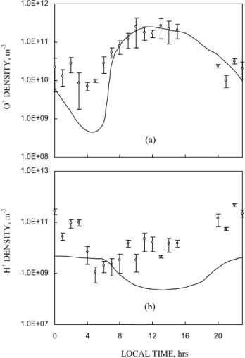
The variation of simulated and observed O+ density, in the June solstice at 10◦N geomagnetic, is shown in Fig. 7a. Diurnal minimum of O+(∼ 7.2 × 10⁹m−3) is observed at
5 1.0E+08 1.0E+09 1.0E+10 1.0E+11 1.0E+12 1.0E+13 0 4 8 12 16 20 1.0E+07 1.0E+09 1.0E+11 1.0E+13 0 4 8 12 16 20 (a) O + DENS ITY, m -3 (b) H + DENS ITY, m -3 LOCAL TIME, hrs Fig. 5. Same as in Fig. 4 for 10◦N geomagnetic latitude.
04:00 LT and the maximum (∼ 2.7 × 10¹¹m−3) at around 13:00 LT. The model fairly simulates the observed density during daytime and evening but gives low values in the pre-sunrise hours. Figure 7b shows the diurnal variation of ob-served and simulated H+density at 10◦N geomagnetic in the same period. The diurnal variation of H+is similar to that at the equator. However, the model predicts slightly lower val-ues than observed in the post noon period. The latitudinal variation of simulated and observed O+ density at the alti-tude of 500 km along the 75◦Indian longitude sector in the December solstice is shown in Fig. 8. It may be noted that measured O+density exhibits a broad peak south of the geo-magnetic equator while simulations reproduced the EIA with peaks at around ±5◦. At other latitudes the simulated and
measured O+density is about the same order.
5 Discussion
Modelling of the low latitude ionosphere has been mostly confined to inputs from the American zone. Vertical E × B drifts used in these models are based on observations for Ji-camarca and Arecibo. Neutral wind, used in these models is also based on ground observations in the American zone or satellite observations having minimum coverage of the
In-1964 P. K. Bhuyan et al.: Theoretical simulation of O+and H+densities 6 1.0E+08 1.0E+09 1.0E+10 1.0E+11 1.0E+12 0 4 8 12 16 20 1.0E+08 1.0E+09 1.0E+10 1.0E+11 1.0E+12 1.0E+13 0 4 8 12 16 20 (a) O + DENS ITY, m -3 (b) H + DENS ITY, m -3 LOCAL TIME, hrs
Fig. 6. Local time variation of measured (o) and simulated (—-) O+ density (a) and H+ density (b) at ∼500 km altitude in the Indian zone over the geomagnetic equator in the June solstice at solar minimum.
dian low latitude region. Use of any of these models may not be consistent with the dynamical processes prevalent in the Indian low latitude region. For present calculations, vertical drifts measured at Trivandrum have been used. It has been observed that the neutral wind model adopted in the present calculation leads to reasonable agreement of calculated and observed parameters. The simulation of ion densities, dur-ing June and December solstices of solar minimum condi-tions within ± 15◦ magnetic latitudes in the Indian longi-tude sector, reproduced the well-known equatorial ionization anomaly at the peak of the F2-layer as seen from measured
NmF2. The model calculations also show the presence of the
EIA for O+, during the December solstice (Fig. 8) within the narrow belt of ± 5◦from the geomagnetic equator, whereas the measured O+at the altitude of 500 km in the Indian zone do not exhibit the anomaly. The total electron density (sum of O+, O+2, NO+, H+, He+densities) during the same pe-riod also shows that at the altitude of 500 km, the ionization peak in the Southern Hemisphere is higher than that in the Northern Hemisphere in the December solstice. Similarly, in the June solstice a broad peak near the equator in the
North-7 1.0E+08 1.0E+09 1.0E+10 1.0E+11 1.0E+12 0 4 8 12 16 20 1.0E+07 1.0E+09 1.0E+11 1.0E+13 0 4 8 12 16 20 (a) O + DENS ITY, m -3 (b) H + DENS ITY, m -3 LOCAL TIME, hrs Fig. 7. Same as in Fig. 6 for 10◦N geomagnetic latitude.
ern Hemisphere has been observed. The average peak height of the F2-layer, during low solar activity in the Indian zone, is about 350 km where the EIA is seen both for measured and simulated density. The E × B drift velocity during solar minimum solstices is relatively weak (Fig. 2) compared to that in the corresponding period of high solar activity. Con-sequently, the plasma fountain fails to reach the altitude re-quired for EIA to be observed at 500 km while producing the effect at the height of peak F2-density. Measurements of electron density made by the Hinotori satellite during 1981– 1982, a period of moderate to high solar activity, within ±25◦magnetic latitudes at 600 km (Watanabe et al., 1995b) indicate a broad ionization peak around the equator during daytime in all seasons. Simulations carried out by Watanabe et al. (1995a) show that maximum in ionization starts devel-oping around the equator at ∼ 10:00 LT and continues until midnight. Balan et al. (1997a), from a study of the equato-rial plasma fountain and equatoequato-rial ionization anomaly in the ionosphere over Jicamarca (77◦E) and Fortaleza (38◦W) us-ing the SUPIM model under magnetically quiet equinoctial conditions of high solar activity, have shown that the EIA is evident up to an altitude of 700 km in the three locations. The EIA is asymmetric about the equator in all the three sectors and has been found to be strongly influenced by the
asym-P. K. Bhuyan et al.: Theoretical simulation of O+and H+densities 1965 8 0 4 8 12 16 20 -10 -5 0 5 10 15 -10 -5 0 5 10 15 0 4 8 12 16 20 -10 -5 0 5 10 15 -10 -5 0 5 10 15
LOCAL TIME, hrs LOCAL TIME, hrs
GEOMAGNET
IC
LATI
TUDE, deg
Fig. 8. Latitudinal and local time variation of observed (left panel)
and simulated (right panel) O+density at an altitude of ∼ 500 km within the geomagnetic latitude range from 10◦S to 15◦N during December solstice of low solar activity.
metric neutral winds and displacement of the geographic and geomagnetic equators. The neutral wind model used in the present simulations might be responsible for the discrepancy between observation and simulation as seen in Fig. 8. The SROSS-C2 satellite orbits covered a latitude belt of 3◦S–
41◦N and a longitude belt of 40◦E–100◦E. The data used
for comparison in this study (Figs. 4–7) are the average of all data at the concerned latitude within the covered longi-tude span of 60◦. Therefore, longitudinal variability may be inherent in the data structure, which may partly be responsi-ble for the scatter in the data points for H+and very low O+ density during morning hours leading to the disagreement between simulation and observation.
6 Conclusion
The diurnal and seasonal variation of O+and H+ densities measured by the SROSS C2 satellite over Indian equatorial and low latitudes at an altitude of 500 km during the low solar activity period of 1995–1996, are simulated by using a time dependent model based on the solution of the plasma conti-nuity equation. The simulated densities are compared with satellite observations for the June and December solstices and with NmF2 measured during the period 1959–1979. Re-sults show that O+ density is minimum in the pre-sunrise
hours and maximum during noontime. H+density exhibits
the opposite diurnal behaviour of high values at night and low values during the day. The O+ density peaks early (∼ 12:00 LT) in the June solstice and late (∼ 14:00 LT) in the December solstice. Simulated and measured NmF2 exhibits the equatorial ionization anomaly. But measured O+density does not show the EIA either in June or December solstice at the altitude of 500 km. The effect of a weak E × B drift in the solstices of low solar activity may be the reason for non-observance of the EIA in O+, which is the major ion at this
altitude. Further studies need to be carried out to investigate this point.
Acknowledgements. This work is supported by a research grant
re-ceived from the Indian Space Research Organization (ISRO). One of the authors (PKK) is grateful to ISRO for providing him a fel-lowship. The authors thank S. C. Garg; Principal Investigator of the SROSS-C RPA project, P. Subrahmanyam and all others involved in the SROSS-C2 data acquisition and analysis program.
Topical Editor M. Lester thanks N. Balan and another referee for their help in evaluating this paper.
References
Anderson, D. N.: A theoretical study of the ionospheric F-region equatorial anomaly-I. Theory, Planet. Space Sci., 21, 409–420, 1973a.
Anderson, D. N.: A theoretical study of the ionospheric F-region equatorial anomaly-II. Results in the American and Asian sec-tors, Planet. Space Sci., 21, 421–442, 1973b.
Anderson, D. N.: Modeling the ambient, low latitude F-region iono-sphere – A review, J. Atmos. Terr. Phys, 43, 753–762, 1981. Bailey, G. J. and Balan, N.: A low latitude ionosphere plasmasphere
model, STEP Handbook of Ionospheric Models, (Ed) Schunk, R. W., Utah State University, Logan, UT 84322-4405, 173–206, 1996.
Bailey, G. J., Balan, N., and Su, Y. Z.: The Sheffield Univer-sity plasmasphere ionosphere model – A review, J. Atmos. Terr. Phys., 59, 1541–1552, 1997.
Bailey, G. J. and Sellek, R.: A mathematical model of the Earth’s plasmasphere and its application in a study of He+ at L = 3, Ann. Geophysicae, 8, 171–190, 1990.
Balan, N., Jayachandran, B., Balachandran Nair, R., Namboothiri, S. P., and Rao, P. B.: HF Doppler observations of vector plasma drifts in the evening F-region at the magnetic equator, J. Atmos. Terr. Phys., 54, 1545–1554, 1992.
Balan, N. and Bailey, G. J.: Equatorial plasma fountain and its ef-fects: Possibility of an additional layer, J. Geiphys. Res., 100, 21 421–21 432, 1995.
Balan, N., Bailey, G. J., Abdu, M. A., Oyama, K. I., Richards, P. G., MacDougall, J., and Batista, I. S.: Equatorial plasma fountain and its effects over three locations: Evidence for an additional layer, the F3-layer, I. S., J. Geophys. Res., 102, 2047–2056, 1997a.
Balan, N., Oyama, K. I., Bailey, G. J., Fukao, S., Watanabe, S., and Abdu, M. A.: A plasma temperature anomaly in the equatorial topside ionosphere, J. Geophys. Res., 102, 7485–7492, 1997b. Baxter, R. G. and Kendall, P. C.: A theoretical technique for
evalu-ating the time dependent effects of general electrodynamic drifts in the F2-layer of the ionosphere, Proc. Roy. Soc. A., 304, 171– 185, 1968.
Bhuyan, P. K. and Kakoty, P. K.: A modelling study of Indian low latitude ionosphere: Part I – Description of the model, Ind. J. Radio. Space Phys., 30, 59–65, 2001a.
Bhuyan, P. K. and Kakoty, P. K.: A modelling study of Indian low latitude ionosphere: Part II – Results and comparison with SROSS C2 satellite data, Ind. J. Radio. Space Phys., 30, 66–71, 2001b.
Bilitza, D.: International Reference Ionosphere-1990 NSSDC 90-22, World Data Center A, Rockets and Satellites, Greenbelt, Md, USA, 1990.
1966 P. K. Bhuyan et al.: Theoretical simulation of O+and H+densities
Bradley P. A. and Dudeney, J. R.: A simple model of the vertical distribution of electron concentration in the ionosphere, J. At-mos. Terr. Phys., 35, 2131–2146, 1973.
Bramley, E. N. and Peart, M.: Diffusion and electromagnetic drift in the equatorial F2-region, J. Atmos. Terr. Phys., 27, 1201–1211, 1965.
Bramley, E. N. and Young, M.: Winds and electromagnetic drifts in the equatorial F2-region, J. Atmos. Terr. Phys., 30, 99–112, 1968.
Chan, H. F. and Walker, G. O.: Computer simulation of the iono-spheric equatorial anomaly in East Asia for equinoctial, solar minimum conditions. Part I – Formulation of model, J. Atmos. Terr. Phys., 46, 1103–1112, 1984a.
Chan, H. F. and Walker, G. O.: Computer simulation of the iono-spheric equatorial anomaly in East Asia for equinoctial, solar minimum conditions. Part II – Results and discussion of wind effects, J. Atmos. Terr. Phys., 46, 1113–1120, 1984b.
Chauhan, N. S. and Gurm, H. S.: Ambipolar diffusion and vertical drift at low-latitudes, Ind. J. Rad. Space Phys., 9, 265–273, 1980. Fejer, B. G.: The equatorial ionospheric electric fields: A review, J.
Atmos. Terr. Phys., 43, 377–386, 1981.
Hanson, W. B. and Moffett, R. J.: Ionization transport effects in the equatorial F-region, J. Geophys. Res., 71, 5559–5572, 1966. Hedin, A. E., MSIS-86 thermospheric model, J. Geophys. Res., 92,
4649–4662, 1987.
Jayachandran, B., Balan., N., Nampoothiri., S. P., and Rao., P. B.: HF Doppler observations of vertical plasma drifts in the evening F-region at the equator, J. Geophys. Res., 92, 11 253–11 256, 1987.
Martyn, D. F.: Atmospheric tides in the ionosphere, I. Solar tides in the F2-region, Proc. R. Soc. London, A189, 241–260, 1947. Millward, G. H., Moffett, R. J., Quegan, S., and Fuller-Rowell,
T. J.: A coupled Thermosphere-Ionosphere-Plasmasphere Model (CTIP), STEP Handbook of Ionospheric Models (Ed) Schunk, R. W., Utah State University, Logan, UT, 84322-4405, 239–272, 1996.
Moffett, R. J.: The equatorial anomaly in the electron distribution of the terrestrial F-region, Fund. Cosmic Phys., 4, 313–391, 1979. Namboothiri, S. P., Balan, N., and Rao, P. B.: Vertical plasma drifts
in the F-region at the magnetic equator, J. Geophys. Res., 94,
12 055–12 060, 1989.
Raitt, W. J., Schunk, R. W., and Banks, P. M.: A comparison of the temperature and density structure in high and low speed thermal proton flow, Planet. Space Sci, 23, 1103–1117, 1975.
Rajaram, G.: Structure of the equatorial F-region topside and bot-tomside – A review, J. Atmos. Terr. phys., 39, 1125–1144, 1977. Rishbeth, H.: Dynamics of the equatorial F-region, J. Atmos. Terr.
Phys., 39, 1159–1168, 1977.
Rishbeth, H.: The equatorial F-layer: progress and puzzles, Ann. Geophysicae, 18, 730–739, 2000.
Rush, C. M.: Ionospheric radio propagation models and predictions – A mini-review, IEEE Trans. Antenn. Propag., AP-34, 1163– 1168, 1986.
St. Maurice, J. P. and Torr, D. G.: Non-thermal rate coefficients in the ionosphere: the reactions of O+with N2, O2and NO, J.
Geophys. Res., 83, 969–976, 1978.
Stening, R. J.: Modeling the low latitude F-region, J. Atmos. Terr. Phys., 54, 1387–1412, 1992.
Sterling, D. L., Hanson, W. B., Moffett, R. J., and Baxter, R. G.: Influence of electromagnetic drifts and neutral air winds on some features of the F2-region, Radio Sci., 4, 1005–1023, 1969. Stubbe, P.: Simultaneous solution of the time-dependent coupled
continuity equations, heat conduction equations and equations of motion for a system consisting of a neutral gas, an electron gas and a four component ion gas, J. Atmos. Terr. Phys., 32, 865– 903, 1970.
Su, Y. Z., Oyama, K. I., Bailey, G. J., Takahashi, T., and Hi-rao, K.: Season, local time and longitude variations of electron temperature measurements at low latitudes with a plasmasphere-ionosphere model, J. Geophys. Res., 100, 14 591–14 604, 1995. Watanabe, S., Oyama, K. I., and Abdu, M. A.: Computer simulation
of electron and ion densities and temperatures in the equatorial F-region and comparison with Hinotori results, J. Geophys. Res., 100, 14 581–14 590, 1995a.
Watanabe, S., Takahashi, T., Oya, H., and Oyama, K. I.: Table of electron density at 600 km altitude during 1981–1982 in the equatorial region, ISAS Research Note, 1995b.
Woodman, R. F.: Vertical drift velocities and east-west electric fields at the magnetic equator, J. Geophys. Res., 75, 6249–6259, 1970.