HAL Id: hal-00629089
https://hal.archives-ouvertes.fr/hal-00629089
Submitted on 13 Feb 2021
HAL is a multi-disciplinary open access
archive for the deposit and dissemination of
sci-entific research documents, whether they are
pub-lished or not. The documents may come from
teaching and research institutions in France or
abroad, or from public or private research centers.
L’archive ouverte pluridisciplinaire HAL, est
destinée au dépôt et à la diffusion de documents
scientifiques de niveau recherche, publiés ou non,
émanant des établissements d’enseignement et de
recherche français ou étrangers, des laboratoires
publics ou privés.
CALIPSO lidar ratio retrieval over the ocean
Damien Josset, Raymond Rogers, Jacques Pelon, Yongxiang Hu, Zhaoyan Liu,
Ali Omar, Peng-Wang Zhai
To cite this version:
Damien Josset, Raymond Rogers, Jacques Pelon, Yongxiang Hu, Zhaoyan Liu, et al.. CALIPSO lidar
ratio retrieval over the ocean. Optics Express, Optical Society of America - OSA Publishing, 2011, 19
(19), pp.18696-18706. �10.1364/OE.19.018696�. �hal-00629089�
CALIPSO lidar ratio retrieval over the ocean
Damien Josset,1,* Raymond Rogers,2 Jacques Pelon,3 Yongxiang Hu,2 Zhaoyan Liu,4 AliOmar,2 and Peng-Wang Zhai1 1SSAI, Hampton, VA 23681
2NASA Langley Research Center, Hampton, VA 23681 3LATMOS, UMR 8190 CNRS / Université Pierre et Marie Curie, France
4NIA, Hampton, VA 23681
Abstract: We are demonstrating on a few cases the capability of CALIPSO
to retrieve the 532 nm lidar ratio over the ocean when CloudSat surface scattering cross section is used as a constraint. We are presenting the algorithm used and comparisons with the column lidar ratio retrieved by the NASA airborne high spectral resolution lidar. For the three cases presented here, the agreement is fairly good. The average CALIPSO 532 nm column lidar ratio bias is 13.7% relative to HSRL, and the relative standard deviation is 13.6%. Considering the natural variability of aerosol microphysical properties, this level of accuracy is significant since the lidar ratio is a good indicator of aerosol types. We are discussing dependencies of the accuracy of retrieved aerosol lidar ratio on atmospheric aerosol homogeneity, lidar signal to noise ratio, and errors in the optical depth retrievals. We are obtaining the best result (bias 7% and standard deviation around 6%) for a nighttime case with a relatively constant lidar ratio (in the vertical) indicative of homogeneous aerosol type.
©2011 Optical Society of America
OCIS codes: (010.0010) Atmospheric and oceanic optics; (280.0280) Remote sensing and
sensors; (280.3640) Lidar; (280.5600) Radar.
References and links
1. F. G. Fernald, B. M. Herman, and J. A. Reagan, “Determination of aerosol height distribution by lidar,” Appl. Opt. 11, 482–489 (1972).
2. J. D. Klett, “Stable analytical inversion solution for processing lidar returns,” Appl. Opt. 20(2), 211–220 (1981). 3. F. G. Fernald, “Analysis of atmospheric lidar observations: some comments,” Appl. Opt. 23(5), 652–653 (1984). 4. S. A. Young and M. A. Vaughan, “The retrieval of profiles of particulate extinction from Cloud Aerosol Lidar
Infrared Pathfinder Satellite Observations (CALIPSO) data: algorithm description,” J. Atmos. Ocean. Technol.
26(6), 1105–1119 (2009).
5. J. Key and A. J. Schweiger, “Tools for atmospheric radiative transfer: Streamer and FluxNet,” Comput. Geosci.
24(5), 443–451 (1998).
6. D. M. Winker, J. Pelon, J. A. Coakley, Jr., S. A. Ackerman, R. J. Charlson, P. R. Colarco, P. Flamant, Q. Fu, R. Hoff, C. Kittaka, T. L. Kubar, H. LeTreut, M. P. McCormick, G. Megie, L. Poole, K. Powell, C. Trepte, M. A. Vaughan, and B. A. Wielicki, “The CALIPSO mission: a global 3d view of aerosols and clouds,” Bull. Am. Meteorol. Soc. 91(9), 1211–1229 (2010).
7. G. L. Stephens, D. G. Vane, S. Tanelli, E. Im, S. Durden, M. Rokey, D. Reinke, P. Partain, G. G. Mace, R. Austin, T. L’Ecuyer, J. Haynes, M. Lebsock, K. Suzuki, D. Waliser, D. Wu, J. Kay, A. Gettelman, Z. Wang, and R. Marchand, “CloudSat mission: performance and early science after the first year of operation,” J. Geophys. Res. 113, D00A18 (2008).
8. D. Josset, J. Pelon, A. Protat, and C. Flamant, “New approach to determine aerosol optical depth from combined CALIPSO and CloudSat ocean surface echoes,” Geophys. Res. Lett. 35(10), L10805 (2008).
9. D. Josset, J. Pelon, and Y. Hu, “Multi-instrument calibration method based on a multiwavelength ocean surface model,” IEEE Geosci. Remote Sens. Lett. 7(1), 195–199 (2010).
10. D. Josset, J. Pelon, Y. Hu, and H. Maring, “Determination of aerosol optical properties using ocean reflectance,” SPIE Newsroom, (2009), http://spie.org/documents/Newsroom/Imported/1574/1574_5743_0_2009-03-19.pdf. 11. J. W. Hair, C. A. Hostetler, A. L. Cook, D. B. Harper, R. A. Ferrare, T. L. Mack, W. Welch, L. R. Izquierdo, and
F. E. Hovis, “Airborne high spectral resolution lidar for profiling aerosol optical properties,” Appl. Opt. 47(36), 6734–6752 (2008).
12. O. Dubovik, A. Sinyuk, T. Lapyonok, B. N. Holben, M. Mishchenko, P. Yang, T. F. Eck, H. Volten, O. Muñoz, B. Veihelmann, W. J. van der Zande, J.-F. Leon, M. Sorokin, and I. Slutsker, “Application of spheroid models to
account for aerosol particle nonsphericity in remote sensing of desert dust,” J. Geophys. Res. 111(D11), D11208 (2006).
13. M. I. Mishchenko and J. W. Hovenier, “Depolarization of light backscattered by randomly oriented nonspherical particles,” Opt. Lett. 20(12), 1356–1358 (1995).
14. R. C. Levy, L. A. Remer, D. Tanre, Y. J. Kaufman, C. Ichoku, B. N. Holben, J. M. Livingston, P. B. Russell, and H. Maring, “Evaluation of the Moderate-Resolution Imaging Spectroradiometer (MODIS) retrievals of dust aerosol over the ocean during PRIDE,” J. Geophys. Res. 108(D19), 8594 (2003).
15. S. G. Howell and B. J. Huebert, “Determining marine aerosol scattering characteristics at ambient humidity from size-resolved chemical composition,” J. Geophys. Res. 103(D1), 1391–1404 (1998).
16. L. D. Mishchenko, Travis, and A. A. Lacis, Scattering, Absorption, and Emission of Light by Small Particles (Cambridge University Press, Cambridge, 2002).
17. C. Bohren and D. Huffman, Absorption and Scattering of Light by Small Particles (Wiley VCH, 1983). 18. O. Dubovik, B. Holben, T. F. Eck, A. Smirnov, Y. J. Kaufman, M. D. King, D. Tanré, and I. Slutsker,
“Variability of absorption and optical properties of key aerosol types observed in worldwide locations,” J. Atmos. Sci. 59(3), 590–608 (2002).
19. A. Keil and J. M. Haywood, “Solar radiative forcing by biomass burning aerosol particles during safari 2000: a case study based on measured aerosol and cloud properties,” J. Geophys. Res. 108(D13), 8467 (2003). 20. M. Hess, P. Koepke, and I. Schult, “Optical properties of aerosols and clouds: the software package OPAC,”
Bull. Am. Meteorol. Soc. 79(5), 831–844 (1998).
21. S. A. Young, “Analysis of lidar backscatter profiles in optically thin clouds,” Appl. Opt. 34(30), 7019–7031 (1995).
22. R. R. Rogers, C. A. Hostetler, J. W. Hair, R. A. Ferrare, Z. Liu, M. D. Obland, D. B. Harper, A. L. Cook, K. A. Powell, M. A. Vaughan, and D. M. Winker, “Assessment of the CALIPSO Lidar 532 nm attenuated backscatter calibration using the NASA LaRC airborne High Spectral Resolution Lidar,” Atmos. Chem. Phys. 11(3), 1295– 1311 (2011).
23. L. A. Remer, Y. J. Kaufman, D. Tanré, S. Mattoo, D. A. Chu, J. V. Martins, R. R. Li, C. Ichoku, R. C. Levy, R. G. Kleidman, T. F. Eck, E. Vermote, and B. N. Holben, “The MODIS aerosol algorithm, products, and validation,” J. Atmos. Sci. 62(4), 947–973 (2005).
24. R. R. Draxler and G. D. Rolph, “HYSPLIT (HYbrid Single-Particle Lagrangian Integrated Trajectory),” (NOAA Air Resouces Laboratory, 2011), http://ready.arl.noaa.gov/HYSPLIT.php.
25. G. D. Rolph, “Real-time Environmental Applications and Display system (READY)” (NOAA Air Resources Laboratory, 2011), http://ready.arl.noaa.gov.
26. S. Tanelli, S. L. Durden, E. Im, K. S. Pak, D. G. Reinke, P. Partain, J. M. Haynes, and R. T. Marchand, “Cloudsat’s cloud profiling radar after two years in orbit: performance, calibration, and processing,” IEEE Trans. Geosci. Rem. Sens. 46(11), 3560–3573 (2008).
27. H. J. Liebe, G. A. Hufford, and M. G. Cotton, “Propagation modeling of moist air and suspended water/ice particles at frequencies below 1000 GHz,” in AGARD, Atmospheric Propagation Effects Through Natural and
Man-Made Obscurants for Visible to MM-Wave Radiation (STI, 1993), pp. 3/1–3/11.
28. A. Omar, D. Winker, C. Kittaka, M. Vaughan, Z. Liu, Y. Hu, C. Trepte, R. Rogers, R. Ferrare, R. Kuehn, and C. Hostetler, “The CALIPSO Automated Aerosol Classification and Lidar Ratio Selection Algorithm,” J. Atmos. Ocean. Technol. 26(10), 1994–2014 (2009).
29. A. Omar, Z. Liu, M. Vaughan, K. Thornhill, C. Kittaka, S. Ismail, Y. Hu, G. Chen, K. Powell, D. Winker, C. Trepte, E. Winstead, and B. Anderson, “Extinction-to-backscatter ratios of Saharan dust layers derived from in situ measurements and CALIPSO overflights during NAMMA,” J. Geophys. Res. 115(D24), D24217 (2010).
1. Introduction
Retrievals of aerosol extinction from a backscatter lidar rely on an inversion procedure [1–4] which is not only limited by the accuracy of the measurements itself, but also by the knowledge of the aerosol microphysical properties (size distribution, shape and refractive indices). These determine the so-called “lidar ratio”, also referred to as the extinction to backscatter ratio. Measurement of extinction vertical profile is important to better understand the aerosol radiative effect and can be directly used as an input of radiative transfer models [5]. We have developed a new methodology based on CALIPSO [6] and CloudSat [7] ocean surface echo to determine the aerosol optical depth (AOD) [8,9] which can be used in combination with CALIPSO vertical backscatter coefficient profiles to retrieve the lidar ratio. In a previous study, we performed a limited retrieval of lidar ratio which was qualitatively consistent with previous values found in the literature [10]. In this paper, we provide a quantitative assessment of the accuracy of our lidar ratio based on a few case studies from coincident underflights with the NASA Langley Research Center (LaRC) airborne High Spectral Resolution Lidar (HSRL), which makes a measurement of the lidar ratio profile [11]. In section 2 we provide the algorithm description. In section 3 we discuss the error sources of the methodology; and finally in section 4 we present the results and provide our assessment of the method, its utility, and limitations.
2. Lidar ratio retrieval
2.1 Lidar ratio definition
If we consider a given set of aerosol particles (subscript p stands for particles), the lidar ratio
p
S (sr) is by definition the ratio of extinction coefficient αp (m
−1) to backscatter coefficient β p
(m−1.sr−1). The double horizontal bar ( ) stands for local parameter defined as the ratio of two quantities weighted by the size distribution.
The size distribution N(D) (m−4) is the number of particles per unit of volume and per unit of a quantity characteristic of the particle size D (m). D is the particle diameter for spherical particles. Noting σext (m2) the extinction cross section, the extinction coefficient is by
definition
0 ( ) ( )
p ext D N D dD
α =
∫
∞σ (1)The backscatter coefficient is a quantity similar to the extinction coefficient but is a function of the scattering cross section σsca (m2) and P11(π) (sr−1) which is the element (1,1) of
the Mueller Matrix [12] at a scattering angle of π radians (i.e. backscatter direction). It represents the total backscattering intensity (sum of the two orthogonal polarization components) for a macroscopically isotropic and mirror-symmetric medium because the backscattering matrix is diagonal under those conditions [13]. When those conditions are not met but the particles are randomly oriented as we would expect for most aerosol observations, the diagonal elements which are not exactly at 0 are small enough to be neglected:
11
0 ( ) ( ) ( )
p P sca D N D dD
β =
∫
∞ π σ (2)The lidar ratio is simply the ratio of Eq. (1) to Eq. (2):
0 11 11 0 ( ) ( ) 1 ( ) ( ) ( ) ( ) ext p p p sca D N D dD S P P D N D dD σ α β π σ ω π ∞ ∞ = =
∫
≡∫
(3)The quantity ωP11( )π is defined by Eq. (3). For a single particle it reduces to a simple product of the single scattering albedo ω defined as the ratio σsca/ σext by P11 but as we can see,
it is in general weighted by the size distribution. Both the single scattering albedo and P11 (and
thus the lidar ratio) are aerosol intensive parameters. They are independent of the amount of aerosol in the atmosphere but are dependent of the aerosol type. Therefore, an accurate determination of lidar ratio from space is expected to help global scale aerosol type discrimination.
The lidar ratio is a local quantity, dependant on the vertical distribution of aerosols properties. We will use a column optical depth as a constraint and will retrieve a column lidar ratio. For a given set of particles, if the atmospheric column boundaries are the top altitude Zt
and the surface altitude Zs, the column lidar ratio S can be defined as p
( ') ' ( ') ' t s t s Z Z p Z Z z dz S z dz α β ⋅ = ⋅
∫
∫
(4)z' is the range where the integration is performed. The horizontal overbar stands for column quantities.
2.2 Expected range of variations of the lidar ratio
Although there is no limitation in the value of the lidar ratio as set by Eq. (3), an estimation of the expected range of variations of this parameter can help to understand the domain of
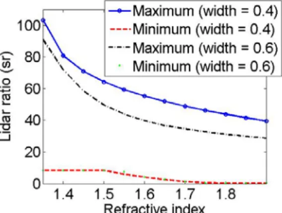
validity of the retrieval. Determining the lidar ratio exact value would require a precise knowledge of the aerosol size distribution as well as its chemical composition, refractive index, and shape. However, a first order estimation does not require all this information. At around 532 nm, the real part of the refractive index can be expected to be between 1.4 for marine aerosols [14] and 1.9 for soot [15]. The size distribution is well represented by a bimodal lognormal size distribution but there is no standard shape. There is in general a well-defined maximum of the extinction efficiency for a specified value of the size parameter, and the lidar ratio will tend to be smaller for a wider size distribution. This maximum is larger for spherical particles than for non-spherical particles [16]. Therefore, using Mie theory [17] with a narrow monomodal lognormal size distribution (width of 0.4 as in [18]) should allow a reasonable (upper range) estimation of the maximum lidar ratio for non-absorbing particles. We report on Fig. 1 the maximum and minimum of the lidar ratio as a function of the refractive index under those conditions at 532 nm when the range of effective particle diameter of the distribution is going from 10−3μm to 10 μm. We are also showing to which extent using a larger size distribution (width of 0.6) lowers the maximum.
Fig. 1. Estimation of the expected maximum and minimum of the lidar ratio for two monomodal lognormal distributions and non-absorbing aerosols. A narrow distribution with a width of 0.4 (solid line for the maximum) and a larger one with a width of 0.6 (solid dotted line for the maximum).
When absorption increases so does the lidar ratio. Values of the single scattering albedo in the range 0.86-0.93 [19] would be expected for biomass burning aerosols. Although there is no limit for absorption, the urban model of [20] is proposing a value of the single scattering albedo not lower than 0.67 and the effect of absorption should on most cases not do more than double the values shown in Fig. 1. Overall, lidar ratio observed in usual conditions should be between 0 sr and much lower than 80-200 sr. Those are extremely high values for spherical particles, narrow monomodal distribution, and highly absorbing particles. In this study, we have set a threshold of 300 sr (to have a supplemental margin due to instrumental noise) and classified higher values of the lidar ratio as unphysical.
2.2 Lidar ratio in the lidar equation formalism
For an atmosphere where molecule scattering is negligible with respect to aerosol scattering, one can find a column particle lidar ratio Sp (sr) which follows the Fernald-Klett equation in
its integrated form. It can be defined as a function of the column particle optical depth τp and
particle column integrated attenuated backscatter Γp (sr−1):
2 1 2 p p p e S τ − − = Γ (5)
It has to be acknowledged that although Sp link with lidar measurements is straightforward
and shown in Eq. (5), only S in Eq. (4) has a real physical meaning. The quantities are p
identical when the lidar ratio is constant on the vertical. We will discuss the agreement between both quantities for the real cases studied here where the lidar ratio can vary in the vertical.
Equation (5) is valid for any wavelength and more specifically can be rewritten as ,532 2 ,532 ,532 1 2 p p p e S τ − − = Γ (6)
Equation (6) is a simple rewriting of Eq. (5) for the wavelength of interest (532 nm). ,532
p
τ is determined by using CALIPSO/CloudSat ocean surface echo and to determine the column particle lidar ratio at 532 nm, Sp,532, we only have to determine the particle column
integrated attenuated backscatter at 532 nm, Γp,532 (sr−1) from CALIPSO data.
2.3 Correction of air molecules scattering in CALIPSO lidar signal
As we are using CALIPSO lidar data, the contribution of air molecules scattering has to be removed to obtain the particle integrated attenuated backscatter at 532 nm. At 1064 nm, the contribution of air molecules is small; much smaller than uncertainties of CALIPSO calibration and optical depth retrieval and it can be neglected. When the contribution of air molecules has to be taken into account the total attenuated backscatter measured by the lidar can be written as 2 ,532( ) ,532( ) tot z tot z e τ β −
(subscript tot for total) [21]: ,532 ,532 2 ( ) ,532 2 ( ) 2 ( ) ,532( ) ,532( ) ,532( ) p tot z z m z tot z e p z m z e e τ τ τ β − =β +β − − (7)
In Eq. (7), z stands for the distance between the lidar and the scatterer. Air density models provided in the CALIPSO data set allows an accurate determination of air molecules backscatter coefficient βm,532 and air molecules (including ozone) optical depth τm,532.
Therefore, the only unknown left to correct the contribution of molecular scattering is the profile of particle optical depth. The advantage of the procedure we are describing in the following is its simplicity and fast computation speed . An iterative procedure as described in [21] is an alternative approach.
We are using the 1064 nm vertical profile shape of attenuated backscatter coefficient as an approximation to determine the 532 nm particle profile shape. To do so, we introduce the quantity
,1064 532
p
S → (sr) in Eq. (8) which is constant on the vertical. This quantity normalized by the lidar ratio at 532 nm represents the wavelength dependency between the two attenuated backscatter coefficient. ,532 2 ,1064 532 ,1064 1 2 p p p e S τ − → − = Γ (8) ,1064 532 p
S → can then be used to scale the 1064 nm channel vertical profile on the 532 nm channel as in Eq. (9): ,532 ,1064 2 ( ) ,1064 532 2 ( ) ,532 ,1064 ,532 ( ) p z p ( ) p z p p p S z e z e S τ τ β − = → β − (9) This allows us to determine the rate of attenuation of molecular scattering by using Eq. (10): ,532 2 ( ) ,532( ) ,532( ) 1 2 ,1064 532 ,1064( ) p z m z e m z Sp p z τ β − β → = − Γ (10)
Simply stated, Eq. (8) to (10) are describing how we use the shape of the attenuated backscatter coefficient at 1064 nm to remove the molecular scattering contribution. An accurate correction is important at lower optical depth and will be discussed in section 3.
At this stage we will be using a shot to shot resolution. Unphysical values of the lidar ratio higher than 300 sr or lower than 0 sr are removed from the data analysis. The 532 nm particle integrated attenuated backscatter will be then retrieved using Eq. (11). Note that we are just using the 1064 nm channel profile shape, and the accuracy of its calibration is not important:
{
2 ,532( ') 2 ,532( ')}
,532 ,532( ') ,532( ') 1 2 ,1064 532 ,1064( ') ' t tot m s Z z z p Z tot z e e m z Sp p z dz τ τ β − β → Γ =∫
− − Γ (11)The integration will be performed between an altitude of 20 km and the surface level around 0 km of altitude. After the shot to shot retrieval, profiles with low level clouds detected by the 333 m and 1 km cloud layer product are removed from the analysis. Both the optical depth and integrated backscatter coefficient will be then averaged at a 20 km horizontal scale (60 shots) using a sliding window. As a final step, we can solve the Fernald-Klett equation, Eq. (6), by using Eq. (11) and the optical depth retrieval determined from CALIPSO/CloudSat ocean surface echo to obtain the lidar ratio at 532 nm.
3. Error analysis
3.1 Generalities
The relative error on the lidar ratio can be derived from Eq. (5) as a function of the error on the column particle optical depth ∆τp and on the particle column integrated attenuated
backscatter ∆Γp (sr−1). 2 2 1 p p p p p p S S eτ τ ∆ ∆ ∆Γ = + Γ − (12)
where ∆Γp is further linked to the errors associated with the CALIPSO lidar calibration and molecular scattering correction. The error due to molecular scattering correction will become noticeable if molecular scattering cannot be neglected with respect to total scattering, that is the potential error will typically increase with lower values of Γp. As the error in that case can become arbitrarily large, this can be detected by a problem of convergence of the lidar ratio retrieval at low optical depth.
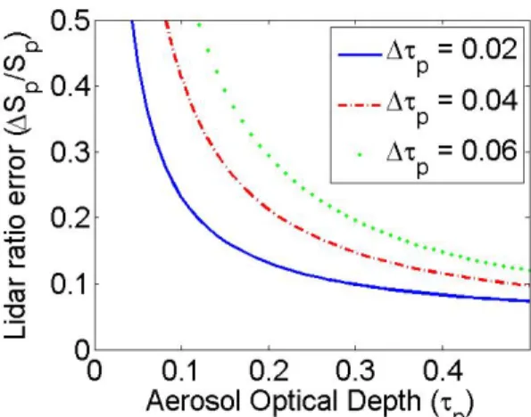
If we take into account an error of 3% in calibration and 2% in the density profile [22], the typical relative error on Γp is probably not lower than 5%. Assuming this 5% error, Eq. (12) can be used to estimate the error on the column retrieval for a given ∆τpand τp.
This is shown in Fig. 2 for different values of ∆τp(0.02, 0.04 and 0.06). As we can see, the
relative error of the retrieval (for a given error on ∆τp) is decreasing with higher optical
thickness. As the average aerosol optical thickness observed over the ocean is of around 0.2 [23], it should not be expected that we can reach an accuracy better than around 20% until extremely high accuracy of calibration and optical thickness retrieval have been reached. However, as we will see, this accuracy already offers the capability to better understand what kind of aerosol are present in the atmospheric column.
Beyond the expected uncertainty, it is important to understand the amount of lidar ratio variations on the vertical as well as the amount of noise in the lidar signal that could potentially affect the retrieval. We have therefore defined two control parameters related to those variations that we will use in our data analysis.
Fig. 2. Expected relative error of the column lidar ratio retrieval as a function of aerosol optical depth for different optical depth error (solid line error of 0.02, solid dotted 0.04 and dotted 0.06).
3.2 Control parameters
3.2.1 SNR*(“simplified 20 km signal to noise ratio”)
The quality of CALIPSO signal is different between day and night and typically lower for optically thin features than for high aerosol load conditions. As we are using a 20 km horizontal average for our retrieval, it is straightforward to estimate the standard deviation of the data within this average. Calculating the real signal to noise ratio would require a careful study of CALIPSO detector characteristics which is beyond the scope of this study and unnecessary to obtain a quantification of the signal quality. It is enough to define a simplified 20 km signal to noise ratio (SNR*) as
,532 ,532 ,532 2 2 * p p p SNR Γ = Γ − Γ (13)
The bracket used in Eq. (13) 〈 〉 stands for the 20 km horizontal sliding window. 3.2.2 lidar ratio Vertical/Column Average Difference (SVCAD)
In order to know to what extent the lidar ratio is constant on the vertical, it is useful to know the absolute average difference between the HSRL vertical lidar ratio measurements and the column lidar ratio. We call it SVCAD (Sp Vertical/Column Average Difference in sr). It is
defined by Eq. (14) as the average difference (in absolute value) between the column lidar ratio and the range resolved measurements.
( ) t s Z p p Z t s S z S dz SVCAD Z Z − = −
∫
(14)This parameter represents the natural variability of the lidar ratio when the detection noise is relatively small (this is the case for the airborne HSRL measurement used in this paper [11]). A totally homogeneous lidar ratio on the vertical would have an SVCAD of 0. For the cases we are showing here, a well-mixed boundary layer aerosol has an SVCAD of around 5 sr (low inhomogeneity) and two different well-defined aerosol layers can create an SVCAD of around 20 sr.
4. Discussion of the results
The NASA LaRC airborne HSRL has generated a large, high quality data set of underflights of the CALIPSO satellite [22]. The methodology described in section 2 is applied to three case studies from HSRL underflights of CALIPSO: 2 nighttime cases, the 9 February 2009 and the 24 August 2010 at around 06:00 UTC, and one daytime case, the 18 August 2010 at around 17:00 UTC. This corresponds respectively to the CALIPSO orbit files timestamps 2009-02-09T06-52-59ZN, 2010-08-24T06-01-41ZN and 2010-08-18T17-19-08ZD.
On February 8th of 2009, the weather in the US Mid-Atlantic states was dominated by a high pressure system. A strong surface temperature inversion confined pollutants in the planetary boundary layer. The Hysplit backtrajectory model [24,25] shows this pollution has been transported during nighttime over the ocean and reached the position where the measurements were taken less than 6h after leaving the east coast. This lead to the observation of pollution over marine boundary layer aerosols for the 9 February case.
The aerosol layers observed the 18th and 24th of August are mainly composed of dust mixed with boundary layer marine aerosols over the Atlantic Ocean. The backtrajectories show the dust leaving the African continent and being advected by the atmospheric circulation during around 8 days and 6 days (respectively) before reaching the Caribbean. The latitude range of those 3 cases are limited by flight duration and by the presence of cirrus clouds. They are respectively 35.7-37.9N, 19.2-22N and 20.9-27N.
In the following, we have used the attenuated backscatter coefficient of CALIPSO level 1 data version 3. The CALIPSO level 2 Cloud Layer 333 m (CAL_LID_L2_333mCLay-ValStage1-V3-01) and 1 km (CAL_LID_L2_01kmCLay-(CAL_LID_L2_333mCLay-ValStage1-V3-01) version 3 cloud products were used to remove low level water clouds from the analysis. This corresponds to the data where clouds were detected at the single–shot resolution (333 m) or after an average of 3 consecutive shots (1 km). The CALIPSO/CloudSat ocean surface optical depth retrieval is based on [8,9]. CloudSat water vapor correction is based on a linear relationship between atmospheric attenuation and AMSR-E integrated water vapor path [26]. The ocean surface product hereafter called Synergized Optical depth of Aerosols (SODA) has been produced for the entire CALIPSO mission data set by the French thematic center of cloud-aerosol-water radiation interactions (ICARE). The shot to shot version of the product has been used in this study.
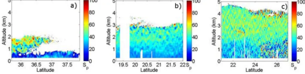
Figure 3 shows the variations of the HSRL aerosol lidar ratio profile as a function of latitude for the three cases presented here. In most cases there is a high level of heterogeneity. The lidar ratio is typically lower than 30 sr in the boundary layer. An upper layer of aerosols is extending a few kilometers above the boundary layer with a much higher lidar ratio, typically between 30 sr and 100 sr. The 24 August case shows less vertical variations of the lidar ratio than the 2 other cases.
Fig. 3. HSRL lidar ratio (Sp in sr) vertical profile as a function of latitude (quicklooks) for the 3 cases of 9 february 2009 (a), 24 August 2010 (b) and 18 August 2010 (c).
Figure 4 shows the column 532 nm aerosol optical depth as retrieved by SODA ocean surface product and the HSRL measurement of the same parameter. The absolute difference between the two retrievals is on average around 0.02 for the first two cases and 0.07 for the 18 August. Although for the first two cases the ocean surface retrieval is extremely accurate considering the current standard of space remote sensing, some improvements should be done to improve the accuracy the 18 August. We are currently investigating if a different
parameterization of the water vapor continuum [27] would improve our retrieval accuracy. Another possibility which could create this AOD underestimation and will be further investigated is the presence of scattered liquid water clouds within CloudSat footprint and not within CALIPSO footprint.
Fig. 4. Optical depth for 3 cases of 9 February 2009 (a), 24 August 2010 (b) and 18 August 2010 (c) determined from the CALIPSO lidar ocean surface return and measured by an airborne HSRL.
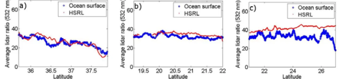
Fig. 5. As in Fig. 4 but showing the column lidar ratio for the 3 cases.
Figure 5 shows the lidar ratio as retrieved by the algorithm described in section 2 and the HSRL column lidar ratio, defined as the ratio of the column integrated extinction and column integrated backscatter coefficient. Overall, the differences observed seem to be related to optical depth differences. This is especially visible for the 24 and 18 August.
Table 1. Characteristics of the three cases presented here
Case 9 February 2009 24 August 2010 18 August 2010
Day/Night Nighttime Nighttime Daytime
Aerosol type Marine and Pollution Marine and dust Marine and dust
Aerosol layer top altitude 2.3 km 3.8 km 4.9 km
Average AOD (HSRL) 0.05 0.29 0.38
Average SNR* 2.3 3.4 2.2
Average SVCAD (HSRL) 13.2 sr 7.8 sr 14.0 sr
Calibration bias +1% +3.4% −1.2%
Average AOD absolute error
−0.02 0.02 0.07
Retrieved Sp 26.3 sr 32.0 sr 33.0 sr
Sp Relative bias −0.5% 7.3% 20.9%
Sp Total relative bias 13.7%
Sp Relative std 15.2% 5.6% 9.8%
Sp Total relative std 13.6%
The main characteristics of the 3 cases are described in Table 1. It contains the average optical depth, the control parameters (SNR* and SVCAD), the level 1 attenuated backscatter calibration relative difference between HSRL and CALIPSO, the average value of retrieved lidar ratio, the relative bias with respect to HSRL of each case, the relative bias of the three cases together, the relative standard deviation of each cases, and all cases together. The differences of calibration are small enough for these three cases to be within the intrinsic uncertainty of comparing airborne and spaceborne measurements (4.5% [22]) and is therefore not a driving issue of the observed differences.
The 9 February 2009 observations are coming from nighttime data but the extremely low optical depth (between 0.025 and 0.12 for SODA) is the sign of a thin features with a low signal to noise ratio (average SNR* around 2.3). As we can see on Fig. 3, the pollution layer is not mixed with the boundary layer. On average, the SVCAD is high. This comes from a regular decrease from around 20 sr in the southern section to 5 sr in the northern section. Due to the low signal to noise ratio and the high lidar ratio vertical inhomogeneity, this is a good test case for our retrieval. Although the inhomogeneity is high, the level of agreement of the lidar ratio is extremely good on overall. The consequence of this low SNR* and vertical inhomogeneity is an important standard deviation of the lidar ratio around 15.2%. The lidar ratio of both HSRL and our methodology decrease southward and the negative bias is around −0.5%. Two explanations are possible to explain the accuracy much higher than what is expected at low optical thickness using Eq. (12). Either there is an error compensation between the different error sources or the accuracy of the optical depth is much higher than what is suggested by the HSRL comparison. This is possible as there are intrinsic differences between airborne and spaceborne observations. Further research will be conducted in the future. At the moment, all we can say is the accuracy is more than acceptable. There is no problem of convergence when the optical depth goes towards 0 and we retrieve a lidar ratio around 14 sr, close from the value of 20 sr, typical of marine boundary layer aerosols [28] even for optical depth lower than 0.03. No problem linked to molecular scattering contribution removal is observed. The average lidar ratio of 26.3 sr is consistent with a mix of marine boundary layer aerosols and pollution.
The case of 24 August also shows a high level of agreement. The combination of nighttime data with a relatively high optical depth (between 0.22 and 0.31 for SODA) induces a high signal to noise ratio (average SNR* around 3.4), favorable for data analysis. Moreover, the lidar ratio is slightly more homogeneous than the previous case (SVCAD around 7.8 sr). As a result, the standard deviation is lower than 6% and the positive bias around 7%.
The case of 18 August is daytime but the high optical depth (between 0.25 and 0.5) corresponds to high aerosol loading, which improves the signal to noise ratio (average SNR* equal to 2.2). The higher positive bias in this case (around 20.9%) is consistent with the higher error on SODA retrieval for this case and an optical depth underestimation.
Overall, for those 3 cases with relatively low optical depth, the optical depth is the driving source of error, as expected from the error budget analysis. This is much more important than all other error sources: molecular scattering correction, vertical homogeneity, and signal to noise ratio. When the optical depth retrieval is accurate, the lidar ratio is in relatively good agreement, even for multi-layer structures and relatively low signal to noise ratio. The average lidar ratio for the 18 and 24 August 2010, respectively 32 sr and 33 sr are slightly lower than the expected lidar ratio at 532 nm for pure dust (slightly lower than 40 sr [29]) and consistent with dust mixed with marine aerosols. As we can see, those values even if not perfectly accurate still provide useful information on the aerosol type.
If we study the distribution of the data for the three cases described here (shown in Fig. 6), the relative bias is 13.7% and the standard deviation 13.6%. The linear correlation
coefficient interpretation is not straightforward. The correlation coefficient between the column HSRL lidar ratio and our retrieval is 0.82 for the 9 February, 0.51 for the 24 August, and −0.31 for 18 August. This is simply because only the first case shows a large range of real geophysical variations of the lidar ratio. For the two other cases, the lidar ratio does not vary much and the correlation coefficient is not a good descriptor because a linear relationship is not formed.
4. Conclusion
We have introduced a simple methodology to retrieve the 532 nm lidar ratio from the SODA data set over the ocean for different aerosol and meteorological conditions, winter and summer, and in day and night lighting conditions. In the three case studies presented here, the column lidar ratios computed with this methodology were quantitatively assessed using underflight data from the airborne HSRL. As expected, high accuracy of optical depth retrieval is a key element of lidar ratio accuracy. Even if it can be improved, our retrieval is reaching a sufficient level of accuracy to increase our knowledge of aerosol types.
The methodology provides better results when the signal to noise ratio is higher. Lidar ratio retrieval accuracy is better for the more homogeneous case but inhomogeneities do not create important problems. The method is fairly robust with no instances of failure to converge or solution instabilities. The results we found will allow improvements in aerosol type discrimination as well as enhancements to the CALIPSO extinction profile retrievals and uncertainty estimates.
Acknowledgments
The CALIPSO NASA project is greatly acknowledged for its support and for funding the HSRL flights as well as CALIPSO NASA/CNES, CloudSat and AMSR-E projects for data availability. The French Thematic center ICARE (http://www.icare.univ-lille1.fr/) is greatly acknowledge for developing and archiving the SODA project. NASA, CNES, Science Systems and Applications Inc. (SSAI) and National Institute of Aerospace (NIA) are greatly acknowledged for their support. The authors gratefully acknowledge the NOAA Air Resources Laboratory (ARL) for the provision of the HYSPLIT transport and dispersion model and READY website (http://www.arl.noaa.gov/ready.php) used in this publication.