HAL Id: hal-00124513
https://hal.archives-ouvertes.fr/hal-00124513
Submitted on 18 Sep 2008
HAL is a multi-disciplinary open access
archive for the deposit and dissemination of
sci-entific research documents, whether they are
pub-lished or not. The documents may come from
teaching and research institutions in France or
abroad, or from public or private research centers.
L’archive ouverte pluridisciplinaire HAL, est
destinée au dépôt et à la diffusion de documents
scientifiques de niveau recherche, publiés ou non,
émanant des établissements d’enseignement et de
recherche français ou étrangers, des laboratoires
publics ou privés.
”Finite-element” displacement fields analysis from digital
images : application to Portevin-Le Châtelier bands
G. Besnard, François Hild, Stéphane Roux
To cite this version:
G. Besnard, François Hild, Stéphane Roux. ”Finite-element” displacement fields analysis from digital
images : application to Portevin-Le Châtelier bands. Experimental Mechanics, Society for
Experimen-tal Mechanics, 2006, 46, pp.789-804. �10.1007/s11340-006-9824-8�. �hal-00124513�
4OR manuscript No. (will be inserted by the editor)
“Finite-element” displacement fields analysis from
digital images:
Application to Portevin-Le Chˆ
atelier bands
Gilles Besnard1,2, Fran¸cois Hild1
, St´ephane Roux2
1 1LMT-Cachan, ENS de Cachan / CNRS-UMR 8535 / Universit´e Paris 6
61 avenue du Pr´esident Wilson, F-94235 Cachan Cedex, France. e-mail: hild@lmt.ens-cachan.fr
2 2Unit´e Mixte CNRS/Saint-Gobain Surface du Verre et Interfaces
39 quai Lucien Lefranc, F-93303 Aubervilliers Cedex, France. e-mail: stephane.roux@saint-gobain.com
The date of receipt and acceptance will be inserted by the editor
Abstract A new methodology is proposed to estimate displacement fields from pairs of images (reference and strained) that evaluates continuous dis-placement fields. This approach is specialized to a finite-element decompo-sition, therefore providing a natural interface with a numerical modeling of the mechanical behavior used for identification purposes. The method is illustrated with the analysis of Portevin-Le Chˆatelier bands in an alu-minum alloy sample subjected to a tensile test. A significant progress with respect to classical digital image correlation techniques is observed in terms of spatial resolution and uncertainty.
Correspondence to: Fran¸cois Hild, Email: hild@lmt.ens-cachan.fr, Fax: +33 1 47 40 22 40.
Keywords: Digital Image Correlation – Localization – Resolution – Tex-ture – Uncertainty.
1 Introduction and motivation
The analysis of displacement fields from mechanical tests is a key ingredient to bridge the gap between experiments and simulations. Different optical techniques are used to achieve this goal (1). Among them, digital image correlation (DIC) is appealing thanks to its versatility in terms of scale of observation ranging from nanoscopic to macroscopic observations with es-sentially the same type of analyses. Most developments based on correlation exploit mainly locally constant or linearly varying displacements (2).
In Solid Mechanics, the measurement stage is only the first part of the analysis. The most important application is the subsequent extraction of mechanical properties, or quantitative evaluations of constitutive law pa-rameters (3). By having an identical description for the displacement field during the measurement stage and for the numerical simulation is the key for reducing the noise or uncertainty propagation in the identification chain. During the latter, there is usually a difference between the kinematic hy-potheses made during the measurement and simulation stages. To avoid this source of noise, it is proposed to develop a DIC approach in which the measured displacement field is consistent with a finite element simulation. Consequently, the measurement mesh has also a mechanical meaning. Let us emphasize that in the present study, only the displacement field mea-surement is considered (i.e., it is a DIC technique), and no (finite-element) mechanical computation is performed. No constitutive law has been chosen, nor any identification performed. However the displacement evaluation is
directly matched to a format ready to use for any further finite element modeling work.
In the following, it is proposed to develop a Q4-DIC technique in which the displacements are assumed to be described by Q4P1-shape functions relevant to finite element simulations (4). The pattern-matching algorithm is based upon the conservation of the optical flow. Variational formulations are derived to solve this ill-posed problem. A spatial regularization was in-troduced by Horn and Schunck (5) and consists in a looking for smooth dis-placement solutions. The quadratic penalization is replaced by “smoother” ones based upon robust statistics (6; 7; 8). In the present approach, the sought displacement field directly satisfies continuity. In its direct applica-tion, the conservation of the optical flow is a non-linear problem that is expressed in terms of the maximization of a correlation product when the sought displacement is piece-wise constant (9). Other kinematic hypotheses are possible and a perturbation technique of the minimization of a quadratic error leads to a linear system as in finite element problems. To increase the measurable displacement range, a multi-scale setting is used as was proposed for a standard DIC algorithm (10).
The paper is organized as follows. Section 2 presents the general princi-ples of a DIC approach. It is particularized to Q4P1-shape functions and is referred to as Q4-DIC. Section 3 is devoted to a performance assessment of the Q4-DIC technique based on a picture of an aluminium alloy sample. This example constitutes a test case, discussed in Section 4, for the quantitative analysis of the kinematics as it offers a good illustration of an heterogeneous strain field (i.e., a localized band is observed in a tensile test).
2 Q4-Digital Image Correlation (Q4-DIC)
In this section the principle of the perturbation approach is introduced. Let us underline that this approach applies to a wide class of functions, and is not confined to finite element shape functions. Other examples have been explored (11; 12), using mechanically based functions, or using spectral decompositions of the displacement field (14; 13). However, the discussion will be specialized to Q4P1-shape functions, which provide a versatile tool for the analysis of very different mechanical problems, ideally suited to finite element modeling.
2.1 Principle of DIC with an arbitrary displacement basis
Let us deal with two images, which characterize the original and deformed surface of a material subjected to a known loading. An image is a scalar function of the spatial coordinate that gives the gray level at each discrete point (or pixel) of coordinate x. The images of the reference and deformed states are respectively called f (x) and g(x). Let us introduce the displace-ment field u(x). This field allows one to relate the two images by requiring the conservation of the optical flow
g(x) = f [x + u(x)] (1)
Assuming that the reference image are differentiable, a Taylor expansion to the first order yields
Let us underline here that the differentiability of the original image is not simply a theoretical question, but we will come back to this point later on. The measurement of the displacement is an ill-posed problem. The dis-placement is only measurable along the direction of the intensity gradient. Consequently, additional hypotheses have to be proposed to solve the prob-lem. If one assumes a locally constant displacement (or velocity), a block matching procedure is found. It consists in maximizing the cross-correlation function (15; 9). To estimate u, the quadratic difference between right and left members of Eq. (2) is integrated over the studied domain Ω and subse-quently minimized η2 = Z Z Ω[u(x).∇f (x) + f (x) − g(x)] 2 dx (3)
The displacement field is decomposed over a set of functions Ψn(x). Each component of the displacement field is treated in a similar manner, and thus only scalar functions ψn(x) are introduced
u(x) =X α,n
aαnψn(x)eα (4)
The objective function is thus expressed as
η2 = Z Z Ω " X α,n aαnψn(x)∇f (x).eα+ f (x) − g(x) #2 dx (5)
and hence its minimization leads to a linear system
X β,m aβm Z Z Ω [ψm(x)ψn(x)∂αf (x)∂βf (x)]dx = Z Z [g(x) − f(x)] ψn(x)∂αf (x)dx (6) that is written in a compact form as
M a= b (7)
where ∂αf = ∇f.eα denotes the directional derivative, the matrix M and the vector b is directly read from Eq. (6)
Mαnβm= Z Z Ω [ψm(x)ψn(x)∂αf (x)∂βf (x)]dx (8) and bαn= Z Z Ω[g(x) − f(x)] ψ n(x)∂αf (x)dx (9)
Let us note that the role played by f and g is symmetric, and up to second order terms, exchanging those two functions will lead to simply ex-changing the sign of the displacement. Thus in order to compensate for variations of the texture and to cancel the induced first order error in u, one substitutes f in the expression of the matrix M by the arithmetic av-erage (f + g)/2. This symmetrization turns out to make the estimate of a much more stable and accurate, although it requires more computation time associated with the assembly of all elementary matrices and vectors.
Last, the present development is similar to a Rayleigh-Ritz procedure frequently used in elastic analyses (4). The only difference corresponds to the fact that the variational formulation is associated to the (linearized) conservation of the optical flow and not the principal of virtual work.
2.2 Particular case: Q4P1-shape functions
A large variety of function Ψ may be considered. Among them, finite element shape functions are particularly attractive because of the interface they
provide between the measurement of the displacement field and a numerical modeling of it based on a constitutive equation. Whatever the strategy chosen for the identification of the constitutive parameters, choosing an identical kinematic description suppresses spurious numerical noise at the comparison step. Moreover, since the image is naturally partitioned into pixels, it is appropriate to choose a square or rectangular shape for each element. This leads us to the choice of Q4-finite elements as the simplest basis. Each element is mapped onto the square [0, 1]2, where the four basic functions are (1 − x)(1 − y), x(1 − y), (1 − x)y and xy in a local (x, y) frame. The displacement decomposition (4) is therefore particularized to account for the previous shape functions of a finite element discretization. Each component of the displacement field is treated in a similar manner, and thus only scalar shape functions Nn(x) are introduced to interpolate the displacement ue(x) in an element Ω
e ue(x) = ne X n=1 X α ae αnNn(x)eα (10)
where ne is the number of nodes (here ne= 4), and aeαn the unknown nodal displacements. The objective function is recast as
η2=X e Z Z Ωe " X α,n aeαnNn(x)∇f (x).eα+ f (x) − g(x) #2 dx (11)
and hence its minimization leads to a linear system (6) in which the matrix M is obtained from the assembly of the elementary matrices Me whose components read
Mαnβme = Z Z
Ωe
and the vector b corresponds to the assembly of the elementary vectors besuch that
beαn= Z Z
[g(x) − f(x)] Nn(x)∂αf (x)dx (13) Thus it is straightforward to compute for each element e the elemen-tary contributions to M and b. The latter is assembled to form the global “rigidity” matrix M and “force” vector b, as in standard finite element prob-lems (4). The only difference is that the “rigidity” matrix nd the “force” vector contain picture gradients in addition to the shape functions, and the “force” vector includes also picture differences. The matrix M is symmet-ric, positive (when the system is invertible) and sparse. These properties are exploited to solve the linear system efficiently. Last, the domain inte-grals involved in the expression of Me and be require imperatively a pixel summation. The classical quadrature formulas (e.g., Gauss point) is not used because of the very irregular nature of the image texture. This latter property is crucial to obtain an accurate displacement evaluation.
2.3 Sub-pixel interpolation
In the previous subsection, the gradient ∇f (x) is used freely in the Taylor expansion leading to Eq. (2). However, f represents the texture of the initial image, discretized at the pixel level. Therefore, the definition of a gradient requires a slight digression. Previous works have underlined the importance of sub-pixel interpolation. In Ref. (16) a cubic spline was argued to be very convenient and precise. Here a different route is proposed, namely, a Fourier decomposition. The latter provides a C∞function that passes by all known values of f at integer coordinates. From such a mapping one easily defines
an interpolated value of the gray level at any intermediate point. Moreover, one also exploits the same mapping for computing a gradient at any point. Finally, powerful Fast Fourier Transform (FFT) algorithms allow for a very rapid computation.
There is however a weakness in this procedure related to the treatment of edges. Fourier transforms over a finite interval implicitly assume periodic-ity. Thus left-right or up-down differences induce spurious oscillations close to edges. To reduce edge effects, each zone of interest (ZOI) is enlarged to an integer power of two size, including a frame around each element. This enlarged ZOI is only used for FFT purposes, and once gradients are esti-mated, the original ZOI is cut out the enlarged zone, and thus the region where most of spurious oscillations are concentrated is omitted. Moreover, at present, an “edge-blurring” procedure is implemented, i.e., each border is replaced by the average of the pixel values of the original and opposite border ones. This again reduces the discontinuity across boundaries (10). There exist a few alternative routes to limit or circumvent part of this arte-fact, namely, ad hoc windowing (10), neutral padding (17), symmetrization, or linear trend removal. Such options have not been tested.
2.4 Multi-scale approach
Even though a way of interpolating between gray level values at a sub-pixel scale was introduced above, the very use of a Taylor expansion requires that the displacement be small when compared with the correlation length of the texture. For a fine texture and a large initial displacement, this requirement appears as inappropriate to converge to a meaningful solution. Thus one may devise a generalization to arbitrarily expand the correlation length of the
texture. This is achieved through a coarse-graining step. Again many ways may be considered, such as a low pass filtering in Fourier or Wavelet spaces. A rather crude, but efficient way, is to resort to a simple coarse-graining in real space (10) obtained by forming super-pixels of size 2n× 2n pixels, by averaging the gray levels of the pixels contained in each super-pixel.
First one generates a set of coarse-grained pictures of f and g for super-pixels of size 2 × 2 super-pixels, 4 × 4 super-pixels, 8 × 8 super-pixels and 16 × 16 super-pixels. Starting from the coarser scale, the displacement is evaluated using the above described procedure. This determination is iterated using a corrected image g where the previously determined displacement is used to correct for the image. These iterations are stopped when the total displacement no longer varies. At this point, one may estimate that a gross determination of the displacement has been obtained, and that only small displacement amplitudes remain unresolved. This lack of resolution is due to the fact that the small scale texture was filtered out. Thus finer scale images are used taking into account the previously estimated displacement to correct for the g image. Again the displacement evaluation is iterated up to convergence. This process is stopped once the displacement is stabilized at the finer scale resolution, i.e., dealing with the original images.
Along the iterations, the “correction” of the deformed image by the pre-viously determined displacement field are possible with different degrees of sophistication. For reasons of computation efficiency, only the most crude correction is performed in the present implementation, namely, each ZOI is simply translated by the average displacement in the element. Integer rounded displacements are taken into account by a mere shift of coordi-nates, and sub-pixel translation is performed by a phase shift in Fourier
space (18). This is a very low cost correction since Fourier transforms are already required to compute gradients.
At the present stage, the implementation is such that the same num-ber of super-pixel is contained in each element. Thus as a finer resolution image is considered, the displacement is to be determined on a physically finer grid. The transfer of the displacement from one scale to the next one is performed using a linear interpolation, consistent with the Q4P1-shape functions that are used. This multi-resolution scheme is thus also a mesh refinement procedure which is performed uniformly (up to now) over the entire map.
This multi-resolution scheme was previously implemented using an FFT-correlation approach to estimate the displacement field (10). In this context, it leads to much more robust results. Large displacements and strains are measured using this algorithm, whereas a single scale procedure revealed to be severely limited. Similarly, using the present Q4-decomposition, this multi-resolution analysis revealed very precious to significantly increase the robustness and accuracy of the measurement.
3 A Priori Performance
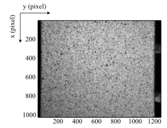
The aim of the present section is to evaluate the a priori performances of the Q4-DIC technique applied to the picture that corresponds to the reference configuration of the experiment to be analyzed in Section 4. Figure 1 shows the texture used to measure displacement fields. It is obtained by spraying a white and black paint prior to the experiment.
3.1 Texture characteristics
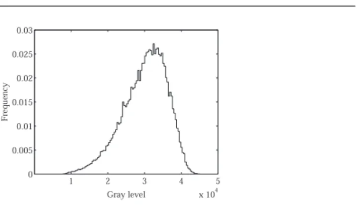
The quality of the displacement measurement is primarily based on the qual-ity of the image texture. Hence before discussing the result of the analysis, the characteristics of the texture are presented. The gray level was encoded on a 16-bit depth (even though the original depth was equal to 12 bits) in the image acquisition, and the true dynamics of gray level takes advantage of this encoding, as judged from the gray level histogram shown in Fig. 2. Such a histogram is a good indication of the global image quality to check for saturation problems.
However, such a global characterization of the image is only of limited interest. What is more significant is the average of texture properties as estimated from sampling of sub-images in ZOIs. The point is to evaluate whether these sub-images carry enough information to allow for a proper analysis. Each ZOI is characterized by its own gray level dynamics, or its standard deviation of gray level. The latter quantity, averaged over all ZOIs of a given size, and normalized by the maximum gray level used in the image, is shown in Fig. 3-a. Even for the smallest ZOI sizes, this ratio is already as large as 0.06, and increases to about 0.13 for large ZOI sizes. The higher the ratio, the smaller the detection threshold as shown in Eq. (2); the standard deviation being an indirect way of characterizing the sensitivity of the technique. One thus concludes that the gray level amplitude is large enough to allow for a good quality of the analysis even for ZOI sizes as small as 4 pixels.
Another significant criterion is the correlation radius of the image tex-ture. The latter is computed from a parabolic interpolation of the auto-correlation function at the origin. The inverse of the two eigenvalues of the
curvature give an estimate of the two correlation radii, ξ1 and ξ2, shown in Fig. 3-b when averaged over all ZOIs of a given size. The texture is rather isotropic (i.e., similar eigenvalues), and remains small (varying from 1-2 to about 3 pixels) for all ZOI sizes. This indicates a very good texture quality that reveals small scale details even for small ZOI sizes. If one wants at least one disk and its complementary surrounding to get a good estimate, the correlation radii should be less than one fourth of the ZOI size. This is achieved for ZOI sizes greater than 6 pixels in the present case.
3.2 Displacement Measurement
Prior to any computation, it is important to estimate the a priori perfor-mance of the approach on the actual texture of the image. If one changes the picture, one may not get exactly the same performance since it is related to the local details of the gray level distribution as shown in Section 2. This is performed by using the original image f only, and generating a trans-lated image g by a prescribed amount upre. Such an image is generated in Fourier space using a simple phase shift for each amplitude. This procedure implies a specific interpolation procedure for inter-pixel gray levels, to which one resorts systematically (see Section 2.3). The algorithm is then run on the pair of images (f, g), and the estimated displacement field uest(x) is measured. One is mainly interested in sub-pixel displacements, where the main origin of errors comes from inter-pixel interpolation. Therefore the pre-scribed displacement is chosen along the (1, 1) direction so as to maximize this interpolation sensitivity. To highlight this reference to the pixel scale, one refers to the x- (or y-) component of the displacement upre ≡ upre.ex
varying from 0 to 1 pixel, rather than the Euclidian norm (varying from 0 to√2 pixels).
The quality of the estimate is characterized by two indicators, namely, the systematic error, δu = khuesti − uprek, and the standard uncertainty σu = hkuest− huestik2i1/2. The change of these two indicators is shown in Fig. 4 as functions of the prescribed displacement amplitude for different ZOI sizes ℓ ranging from 4 to 128 pixels. Both quantities reach a maximum for one half pixel displacement, upre= 0.5 pixel, and are approximately sym-metric about this maximum. Integer valued displacements (in pixels) imply no interpolation and is exactly captured through the multi-scale procedure discussed above. This confirms that these errors are due to interpolation procedures. The results are shown in a semi-log scale to reveal the strong sensitivity to the ZOI size, however a linear scale would show that both δu and σu follow a linear increase with upre from 0 to 0.5 pixel (and a symmetric decrease from 0.5 to 1 pixel).
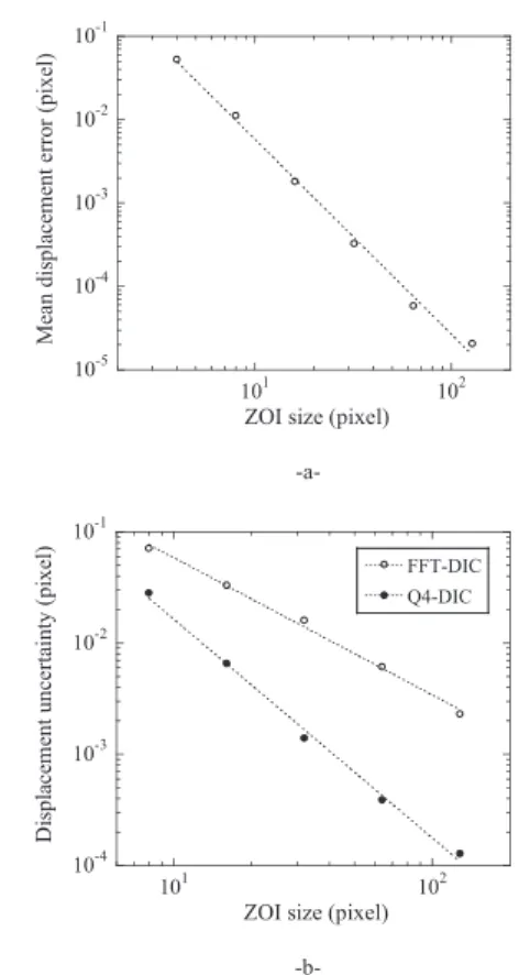
To quantify the effect of the ZOI size, the error and standard uncertainty, are averaged over uprewithin the range [0, 1] as functions of the ZOI size ℓ. These data are shown in Fig. 5. A power-law decrease
hσui = A1+ζℓ−ζ hδui = B1+υℓ−υ
(14) for 8 ≤ ℓ ≤ 128 pixels is observed as shown by a line on the graph. Both amplitudes are close to 1 pixel (more precisely A = 1.15 pixel and B = 1.07 pixel). The exponents are measured to be ζ = 1.96 and υ = 2.34. The data for ℓ = 128 pixels seem to depart from the power-law
For comparison purposes, the displacement uncertainties obtained with the present technique are compared with those of a standard FFT-DIC
technique (10). In that case, a weaker power-law decrease is observed with A = 1.00 pixel and ζ = 1.23 (Fig. 5b). This result shows that by using a con-tinuous description of the displacement field, it enables for a decrease of the displacement uncertainty when the same ZOI size is used. Conversely, for a given displacement uncertainty, the Q4-DIC algorithm allows one to reduce significantly the ZOI size, thereby increasing the number of measurement points when compared to a classical FFT-DIC technique.
3.3 Noise sensitivity
Last, the effect of noise associated to the image acquisition (e.g., digiti-zation, read-out noise, black current noise, photon noise (19)) on the dis-placement measurement is assessed. This analysis allows one to estimate the displacement resolution (20). The reference image is corrupted by a Gaussian noise of zero mean and standard variation σg ranging from 1 to 8 gray levels at each pixel with no spatial correlation. No displacement field is superimposed on the image, and the displacement field is then estimated. The standard deviation of the displacement field, σu, is shown in Fig. 6 as a function of the noise amplitude σg and for different ZOI sizes ranging from 4 to 128 pixels. The quantity σu is linear in the noise amplitude and in-versely proportional to the ZOI size. The latter properties are derived from the central limit theorem.
A theoretical analysis of this problem is discussed in Ref. (11) and sum-marized in the Appendix, and leads to the following estimate of the standard deviation of the displacement field induced by a Gaussian white noise
σu=
12√2σgp
where p is the physical pixel size. For the present application, one com-putes h|∇f|2
i1/2 ≈ 5340 pixel−1, hence σ
u ≈ 4.5 × 10⁻⁴σgp/ℓ. This theo-retical expectation (neglecting the spatial correlation in the image texture) is consistent with the direct estimates shown in Fig. 6 (e.g., for ℓ = 4 pixels and σg = 8 gray levels, the direct estimate is 1.2 × 10−3 pixel to be com-pared with 9 × 10−4pixel given by the above formula). In practice, with the used CCD camera, the noise level is given with a maximum range less than 3 gray levels. Consequently, the contribution of image noise is negligibly small when compared to that induced by the sub-pixel interpolation.
4 Application to a tensile test
In this section, an application of the previously proposed algorithm is carried out to analyze a tensile test performed on an aluminum alloy sample. In the plastic regime, the formation of localization strain bands are observed. The fact that for a given the displacement uncertainty, smaller ZOI sizes can be chosen in the present case (Q4-DIC) when compared with those of a standard FFT-DIC technique (Fig. 5b), enables one to better capture kinematic details in the localization band.
4.1 Material and method
The studied aluminum alloy is of type 5005 (i.e., more than 99 wt% of Al content and a small amount of Mg; these values were determined by elec-tron probe micro-analysis). As shown in Fig. 1, the sample is a coated with sprayed black and white paints to create the random texture for the dis-placement field measurement. The sample size is 140 × 30 × 2 mm3. It is
positioned within hydraulic grips of a 100 kN servo-hydraulic testing ma-chine. Its alignment is checked with DIC measurements (i.e., no significant rotation of the sample is observed in the elastic domain). To have a first strain evaluation, an extensometer was used. Its pins are observed on the right edge of the sample (Fig. 1).
An artificial light source is used to minimize gray level variations so that the conservation of the optical flow is considered as practically achieved. A CCD camera (12-bit digitization, noise less than 3 gray levels, resolution: 1024 × 1280 pixels) with a conventional zoom is positioned in front of the sample. In the present case, the physical size of one pixel is 25 µm. Two loading sequences are carried out. First, in the elastic domain, a controlled displacement rate of 5 µm/s is applied and pictures are taken for 12 µm-increments. Elastic properties may be identified (21). This will not be dis-cussed herein. Second, a controlled displacement rate of 10 µm/s is applied to study strain localization and pictures are taken for 60 µm-increments. The following analysis of the displacement field is an increment between two image acquisitions in the “plastic” regime.
Figure 7 shows the change of the average longitudinal strain with the number of pictures (or equivalently with time). This result was obtained by using the Q4-DIC analysis. Until the extensometer pins slipped (at about a 5% strain), the average strain measured by DIC and that given by the extensometer were close, even though the same surface was not analyzed. This response is typical of a Portevin-Le Chˆatelier (PLC) phenomenon or jerky flow (22). From a microscopic point of view, PLC effects are related to dynamic interactions between mobile dislocations and diffusing solute atoms (23; 24). From a macroscopic perspective, it is related to a negative
strain rate sensitivity that leads to localized bands that are simulated (25). Many experimental studies (26) however are based upon average strain mea-surements. There are also full-field displacement measurements performed by using, for instance, laser speckle interferometry (27). Yet the spatial res-olution did not allow for an analysis of the displacement field within the band. Additional insight is gained by using IR thermography (28).
4.2 Kinematic fields
Let us now analyze the displacement field in between two states (0.3% mean strain apart, see Fig. 7). The same region of interest of size 1000 ×700 pixels is studied using the above method, with different ZOI sizes ranging from 16 down to 4 pixels. Figures 8 and 9 show the resulting displacement fields (component Uxand Uy, respectively). Although the test is pure tension, the analysis reveals without ambiguity the presence of a localization band whose width is about 150 pixels, and across which the displacement discontinuity is about 2 pixels along the tension axis, and about 1 pixel perpendicular to it. The mechanical analysis of this PLC localization phenomenon based on kinematic as well as thermographic images is deferred to a further publica-tion. Let us concentrate here on this single pair of images to validate the algorithm on a real experimental test and evaluate its performances.
One notes that all ZOI sizes may be used. As expected, the smallest ZOI sizes are noisier, yet the agreement between all these determinations is excellent. Let us underline that FFT-DIC usually deals with ZOI sizes equal or larger than 32 pixels, exceptionally 16 pixels for very favorable cases are used when locally constant displacement fields are sought. Using the Q4-DIC technique allows one to reduce the ZOI size by a factor of 4,
which means that the number of pixels in the ZOI has been cut down by a factor of 16.
Let us however note that one should be cautious about the fact that dis-placements have a tendency to be attracted toward integer values, especially for small ZOI sizes. Therefore the direct evaluation of strains along the ten-sion axis εyy as obtained by the Q4P1-shape functions or equivalently as a simple finite difference is expected to be artificially increased at half-integer displacement components. Figure 10 shows such strain fields for 4 different ZOI sizes from 16 down to 8 pixels. For a size of 16 pixels, the localization band appears as a genuine zone of increased strains as compared to a “silent” (or elastic) background. For smaller ZOI sizes, the edges of the shear band appear to concentrate still a higher strain. The same effect is apparent for ZOI sizes 12, 10 and 8 pixels. The strain maps obtained for smaller ZOI sizes are not shown, since the noise level becomes much higher and thus the measurement cannot be trusted. The same artefact of strain enhancement at the edges of the shear band is however observed.
4.3 Integer locking
One notes on the previous figure that the Uy-displacement is half-integer valued at the edge of the shear band. The larger strains at the edge of the band could therefore be interpreted as an artefact due to integer locking. Integer valued displacements being favored, an artificial gap is created for half-integer values displacement, and thus any gradient (finite difference operator) will underline this effect very markedly.
To test this interpretation, the following test is proposed. An artificially translated image by 0.5 pixel is computed from the original one, using a fast
Fourier transform, as the latter provides a simple and numerically efficient way of interpolating the image at any arbitrary sub-pixel value. A genuine strain enhancement is thus expected to be identified at a fixed position in the reference image frame of coordinates, whereas a numerical artefact would be moved to a different location. Figures 11a and b show the Uy displacement component starting from the original image or from the translated one (and where the 1/2 pixel translated has been corrected for). A good agreement is observed for the displacement field thus revealing a rather poor sensitivity to such a rigid translation. Figures 11c and d show the corresponding εyy strain maps. On the latter set of figures, although high strain values tend to concentrate along two lines in both figures, the precise location of these bands is not stable. This is a signature of the integer locking phenomenon. Therefore the strain enhancement at the edge of the shear band is to be considered as an artefact.
Let us underline that such a phenomenon results from the fact that the zones of interest are reduced to a very small size, and still provide a very accurate determination of the displacement field, without much noise. Such a success encourages the user to decrease the size of the zone of interest to very small values. By doing so, the determination of the displacement is much more prone to slight sub-pixel shifts (Fig. 5), here characterized as an attraction toward integer values, which appear as very significant upon differentiation (in the computation of the strain). This phenomenon should be identified before any further interpretation of the strain map to ensure its validity.
4.4 Error maps
As mentioned earlier, a very important output of the displacement mea-surement obtained from a minimization procedure is that the optimization functional provides not only a global quality factor of the determined field, but more importantly a spatial map of residuals, so that one may appreciate a specific problem that may be spatially localized.
Figure 12 shows the different error maps obtained for different ZOI sizes. This error is the remanent difference in gray levels that is still unexplained by the estimated displacement field. The first observation is that the error level does not very much with the ZOI size. This is consistent with the fact that the displacement field is quite comparable for different ZOI sizes. However, there is a slight increase in the error as the ZOI size decreases. This is explained by the fact that the performance of the correlation algorithm degrades as the spatial resolution improves. This observation is in good agreement with the results to be expected from the analysis of Fig. 5.
5 Conclusion
A novel approach was developed to determine a displacement field based on the comparison of two digital images. The sought displacement field is de-composed onto a basis of continuous functions using Q4P1-shape functions as proposed in finite element methods. The latter corresponds to one of the simplest kinematic descriptions. It therefore allows for a compatibility of the kinematic hypotheses made during the measurement stage and the sub-sequent identification / validation stage, for instance, by using conventional finite element techniques.
The performance of the algorithm is tested on a reference image to eval-uate the reliability of the estimation, which is shown to allow for either an excellent accuracy for homogeneous displacement fields, or for a very well resolved displacement field down to element sizes as small as 4×4 pixels. When compared with a standard FFT-DIC technique, Q4-DIC enables for a significant decrease of the displacement uncertainty when the same size of the zone of interest is used.
Last, the displacement field is analyzed on an aluminium alloy sample where a localization band develops. In the present case, it corresponds to a Portevin-Le Chˆatelier effect. For element sizes ranging from 16 down to 4 pixels, the displacement field is shown to be reliably determined. As far as strains are concerned, spurious strain concentrations at the edge of the shear band is observed for small element sizes. This is attributed to integer locking of the displacement. Apart from this bias, the analysis has been shown to be operational and reliable, on a real experimental test with strain localization. The complete space-time kinematic analysis is now possible for the Portevin-Le Chˆatelier phenomenon even within the band thanks to the spatial resolution achieved by the Q4-DIC technique presented herein. It is deferred to a another publication.
Acknowledgments
The authors acknowledge useful discussions with Prs. A. Benallal and J. Lemaitre. This work is part of a project (PHOTOFIT) funded by the Agence Nationale de la Recherche.
References
P. K. Rastogi, edts., Photomechanics, (Springer, Berlin (Germany), 2000), 77. M. A. Sutton, S. R. McNeill, J. D. Helm and Y. J. Chao, Advances in Two-Dimensional and Three-Dimensional Computer Vision, in: Photomechanics, P. K. Rastogi, eds., (Springer, Berlin (Germany), 2000), 323-372.
A. Lagarde, edt., Advanced Optical Methods and Applications in Solid Mechanics, (Kluwer, Dordrecht (the Netherlands), 2000), 82.
O. C. Zienkievicz and R. L. Taylor, The Finite Element Method, (McGraw-Hill, London (UK), 4th edition, 1989).
B. K. P. Horn and B. G. Schunck, Determining optical flow, Artificial Intelligence 17 (1981) 185-20.
P. J. Hubert, Robust Statistics, (Wiley, New York (USA), 1981).
M. Black, Robust Incremental Optical Flow, (PhD dissertation, Yale University, 1992). J.-M. Odobez and P. Bouthemy, Robust multiresolution estimation of parametric motion models, J. Visual Comm. Image Repres. 6 (1995) 348-365.
M. A. Sutton, W. J. Wolters, W. H. Peters, W. F. Ranson and S. R. McNeill, Deter-mination of Displacements Using an Improved Digital Correlation Method, Im. Vis. Comp. 1 [3] (1983) 133-139.
F. Hild, B. Raka, M. Baudequin, S. Roux and F. Cantelaube, Multi-Scale Displacement Field Measurements of Compressed Mineral Wool Samples by Digital Image Correlation, Appl. Optics IP 41 [32] (2002) 6815-6828.
S. Roux and F. Hild, Stress intensity factor measurements from digital image correlation: post-processing and integrated approaches, Int. J. Fract. [in press] (2006).
F. Hild and S. Roux, Digital Image Correlation: From Displacement Measurement to Identification of Elastic Properties - A Review, Strain [in press] (2006).
B. Wagne, S. Roux and F. Hild, Spectral Approach to Displacement Evaluation From Image Analysis, Eur. Phys. J. AP 17 (2002) 247-252.
S. Roux, F. Hild and Y. Berthaud, Correlation Image Velocimetry: A Spectral Approach, Appl. Optics 41 [1] (2002) 108-115.
P. J. Burt, C. Yen and X. Xu, Local correlation measures for motion analysis: a com-parative study, Proceedings IEEE Conf. on Pattern Recognition and Image Processing, (1982), 269-274.
H. W. Schreier, J. R. Braasch and M. A. Sutton, Systematic errors in digital image correlation caused by intensity interpolation, Opt. Eng. 39 [11] (2000) 2915-2921.
S. Bergonnier, F. Hild and S. Roux, Local anisotropy analysis for non-smooth images, Patt. Recogn. [in press] (2006).
J.-N. P´eri´e, S. Calloch, C. Cluzel and F. Hild, Analysis of a Multiaxial Test on a C/C Composite by Using Digital Image Correlation and a Damage Model, Exp. Mech. 42 [3] (2002) 318-328.
G. Holst, CCD Arrays, Cameras and Displays, (SPIE Engineering Press, Washington DC (USA), 1998).
ISO, International Vocabulary of Basic and General Terms in Metrology (VIM), (In-ternational Organization for Standardization, Geneva (Switzerland), 1993).
G. Besnard, Corr´elation d’images et identification en m´ecanique des solides, (University Paris 6, Intermediate MSc report 2005).
A. Portevin and F. Le Chˆatelier, C. R. Acad. Sci. Paris 176 (1923) 507. A. H. Cottrell, Phil. Mag. 44 (1953) 829.
P. G. McCormick, Acta Metall. 20 (1972) 351.
A. H. Clausen, T. Borvik, O. S. Hopperstad and A. Benallal, Flow and fracture charac-teristics of aluminium alloy AA5083-H116 as function of strain rate, temperature and triaxiality, Mat. Sci. Eng. A364 (2004) 260-272.
D. Thevenet, M. Mliha-Touati and A. Zeghloul, Characteristics of the propagating de-formation bands associated with the Portevin-Le Chˆatelier effect in an Al-Zn-Mg-Cu alloy, Mat. Sci. Eng. A291 (2000) 110-117.
R. Shabadi, S. Kumara, H. J. Roven and E. S. Dwarakadasa, Characterisation of PLC band parameters using laser speckle technique, Mat. Sci. Eng. A364 (2004) 140-150. H. Louche, P. Vacher and R. Arrieux, Thermal observations associated with the Portevin-Le Chˆatelier effect in an Al-Mg alloy, Mat. Sci. Eng. A 404 (2005) 188-196.
Appendix: Sensitivity to image noise
The sensitivity of the displacement evaluation to noise is addressed. It is assumed that the deformed image is corrupted by a random white noise ρ, of zero mean, and variance σ2
g. The notations of Section 2 are used. The M matrix is thus unaffected by this noise, but only the vector b is modified by a quantity
δbn= Z Z
ρ(x).(∇f.Ψn)dx (16)
On average, hδbi = 0, and
hδbmδbni = σg2Mmn (17) The impact of this noise on the determination of a, which is not altered by a fluctuating part δa, is sought. By linearity, one observes that hδai = 0. Its variance is given by
hδamδani = σg2M −1 mpM −1 nqMpq= σ2gM −1 mn (18)
Rather than computing the exact above estimate of the variance of the displacement field (the M−1
matrix is quite large), one further simplifies the computation, and only consider the spatial average of the covariance matrix hδamδani. This hypothesis ignores the edge effects where the variance will be larger than within the domain. It also exploits the assumption that the gradient of the image has only short distance correlations as compared to the Q4-element size. The average symbol h...i is now understood as representing an ensemble average over the noise, and a spatial average. As a result the matrix M has to be averaged, and reads
hMmni = (1/2)h|∇f|2i Z Z
Ψm.Ψndx (19)
The interesting feature of this equation is the fact that only the shape functions are involved in the integral. This results in a natural decoupling between the x and the y coordinates of the displacement, and a quasi-band diagonal of this function inherited from the classical finite-element formulation. For instance, the diagonal elements will have the following expression
hMnni = (2/9)h|∇f|2iℓ2 (20) for a summation performed over the 4 elements attached to this node. For two adjacent nodes, hMmni = (1/9)h|∇f|2iℓ2, and for two diagonally opposed nodes, hMnni = (1/36)h|∇f|2iℓ2. This matrix is easily inverted. It has the same support as M . The diagonal element is
hMi−1
nn =
288
49h|∇f|2iℓ2 (21)
The adjacent node matrix element is −(1/4) that value, and diagonally opposed nodes are 1/16 of it. By making a final additional hypothesis that the inverse of the spatial average is identified with the spatial average of the inverse (i.e., valid for a homogeneous texture of the image), the final expression of the standard deviation σa of the Q4-displacement amplitude is expressed as
σa=phδa2ni =
12√2pσg
It is to be noted that the fluctuating part of the a field is anti-correlated. Thus part of the fluctuations at one node is compensated by the fluctuations on neighboring nodes.
200 400 600 800 1000 1200 200 400 600 800 1000 y (pixel) x (pixel)
Fig. 1. View of the reference image. The tension axis is vertical. The width of the sample is 30 mm.
1 2 3 4 5 x 10⁴ 0 0.005 0.01 0.015 0.02 0.025 0.03 Gray level Frequenc y
2 4 8 16 32 64 1.0 1.5 2.0 2.5 3.0 3.5
ZOI size (pixel) x (pixel) 2 4 8 16 32 64 0.06 0.07 0.08 0.09 0.1 0.11 0.12 0.13 M ean gray le vel fl uctuat ion
ZOI size (pixel)
-a-Fig. 3. Fluctuation of gray level values averaged over ZOI of different sizes normalized by the dynamics of gray levels of the image (a). Average of largest (+) and smallest (◦) correlation radii determined on ZOIs of varying sizes (b).
10-6 10-5 10-4 10-3 10-2 10-1 0 0.2 0.4 0.6 0.8 1 4 8 16 32 64 128
Prescribed displacement (pixel)
-a-M ea n d is p la ce m en t er ro r (p ix el ) 10-5 10-4 10-3 10-2 10-1 100 0 0.2 0.4 0.6 0.8 1 4 8 16 32 64 128 S ta n d ar d u n ce rt ai n ty ( p ix el )
Prescribed displacement (pixel)
-b-Fig. 4. Mean error δuand standard deviation σu as a function of the prescribed
10-5 10-4 10-3 10-2 10-1 101 102 M ea n d is p la ce m en t er ro r (p ix el )
ZOI size (pixel) -a-10-4 10-3 10-2 10-1 101 102 FFT-DIC Q4-DIC D isp la ce m en t u n ce rt ai n ty ( p ix el )
ZOI size (pixel)
-b-Fig. 5. Average error hδui and standard uncertainty hσui as functions of the ZOI size
ℓ. For the displacement uncertainty, the results obtained by Q4-DIC are compared with those obtained by FFT-DIC. The dashed lines correspond to power-law fits.
0 2 4 6 8 0
0.5 1 1.5x 10
Noise level (gray level)
Standard uncertainty (pixel)
4 8 16 32 64 128 -3
Fig. 6. Standard deviation of the displacement error versus noise amplitude for different ZOI sizes (4, 8, 16, 32, 64 and 128 pixels) from top to bottom.
0 0.01 0.02 0.03 0.04 0.05 0.06 0.07 0 20 40 60 80 100 120 140 Mean strain Picture number
Fig. 7. Mean strain for a region of interest of 1000 × 700 pixels as a function of the number of picture. The box shows the two pictures that are analyzed.
y (pixel) x (pixel) 200 400 600 -a-800 1000 100 200 300 400 500 600 700 800 200 400 600 -b-800 1000 100 200 300 400 500 600 700 800 200 400 600 -c-800 1000 100 200 300 400 500 600 700 800 0.6 0.4 0.2 0 0.2 0.4 U y (pixel) 200 400 600 -d-800 1000 100 200 300 400 500 600 700 800 200 400 600 -e-800 1000 100 200 300 400 500 600 700 800 200 400 600 -f-800 1000 100 200 300 400 500 600 700 800
Fig. 8. Map of Uydisplacement for different ZOI sizes: (a) ℓ = 16, (b) ℓ = 12, (c) ℓ = 10,
200 400 600 -a-800 1000 100 200 300 400 500 600 700 800 U x (pixel) 200 400 600 -b-800 1000 100 200 300 400 500 600 700 800 200 400 600 -c-800 1000 100 200 300 400 500 600 700 800 0 0.5 1 1.5 2 y (pixel) x (pixel) 200 400 600 -d-800 1000 100 200 300 400 500 600 700 800 200 400 600 -e-800 1000 100 200 300 400 500 600 700 800 200 400 600 -f-800 1000 100 200 300 400 500 600 700 800
Fig. 9. Map of Uxdisplacement for different ZOI sizes: (a) ℓ = 16, (b) ℓ = 12, (c) ℓ = 10,
200 400 600 -a-800 1000 100 200 300 400 500 600 700 800 200 400 600 -b-800 1000 100 200 300 400 500 600 700 800 200 400 600 -c-800 1000 100 200 300 400 500 600 700 800 0.015 0.01 0.005 0 0.005 0.01 0.015 0.02 0.025 εxx y (pixel) x (pi xel) 200 400 600 -d-800 1000 100 200 300 400 500 600 700 800
Fig. 10. Map of the strain component εxxfor different ZOI sizes: (a) ℓ = 16, (b) ℓ = 12,
200 400 600 -a-800 1000 100 200 300 400 500 600 700 800 2 1.5 1 0.5 0 Ux (pixel) 200 400 600 -b-800 1000 100 200 300 400 500 600 700 800 200 400 600 -c-800 1000 100 200 300 400 500 600 700 800 0.04 0.03 0.02 0.01 0 0.01 0.02 0.03 0.04 ε xx y (pixel) x (pixel) 200 400 600 -d-800 1000 100 200 300 400 500 600 700 800
Fig. 11. Map of Uxdisplacement,estimated for a ZOI size ℓ = 12 pixels: (a) for the
orig-inal image, (b) for an artificially translated image of 0.5 pixel. Maps of the corresponding normal strain component εxx: (c) for the original image, (d) for an artificially translated
Fig. 12. Map of the residual error η for different ZOI sizes: (a) ℓ = 16, (b) ℓ = 12, (c) ℓ= 10 (d) ℓ = 8, (e) ℓ = 6 and (f) ℓ = 4 pixels.