HAL Id: insu-02498516
https://hal-insu.archives-ouvertes.fr/insu-02498516
Submitted on 4 Mar 2020
HAL is a multi-disciplinary open access
archive for the deposit and dissemination of
sci-entific research documents, whether they are
pub-lished or not. The documents may come from
teaching and research institutions in France or
abroad, or from public or private research centers.
L’archive ouverte pluridisciplinaire HAL, est
destinée au dépôt et à la diffusion de documents
scientifiques de niveau recherche, publiés ou non,
émanant des établissements d’enseignement et de
recherche français ou étrangers, des laboratoires
publics ou privés.
Possible Effects of Greenhouse Gases to Ozone Profiles
and DNA Active UV-B Irradiance at Ground Level
Kostas Eleftheratos, John Kapsomenakis, Christos Zerefos, Alkiviadis Bais,
Ilias Fountoulakis, Martin Dameris, Patrick Jöckel, Amund Haslerud, Sophie
Godin-Beekmann, Wolfgang Steinbrecht, et al.
To cite this version:
Kostas Eleftheratos, John Kapsomenakis, Christos Zerefos, Alkiviadis Bais, Ilias Fountoulakis, et al..
Possible Effects of Greenhouse Gases to Ozone Profiles and DNA Active UV-B Irradiance at Ground
Level. Atmosphere, MDPI 2020, 11 (3), pp.228. �10.3390/atmos11030228�. �insu-02498516�
Atmosphere 2020, 11, 228; doi:10.3390/atmos11030228 www.mdpi.com/journal/atmosphere Article
Possible Effects of Greenhouse Gases to Ozone
Profiles and DNA Active UV‐B Irradiance at
Ground Level
Kostas Eleftheratos 1,2,*, John Kapsomenakis 3, Christos S. Zerefos 2,3,4, Alkiviadis F. Bais 5, Ilias Fountoulakis 5,6, Martin Dameris 7, Patrick Jöckel 7, Amund S. Haslerud 8,
Sophie Godin‐Beekmann 9, Wolfgang Steinbrecht 10, Irina Petropavlovskikh 11,
Colette Brogniez 12, Thierry Leblanc 13, J. Ben Liley 14, Richard Querel 14 and Daan P. J. Swart 15
1 Department of Geology and Geoenvironment, National and Kapodistrian University of Athens, 15784 Athens, Greece 2 Center for Environmental Effects on Health, Biomedical Research Foundation of the Academy of Athens, 11527 Athens, Greece; zerefos@geol.uoa.gr 3 Research Centre for Atmospheric Physics and Climatology, Academy of Athens, 10680 Athens, Greece; johnkaps@geol.uoa.gr 4 Navarino Environmental Observatory (N.E.O), 24001 Messinia, Greece 5 Department of Physics, Aristotle University of Thessaloniki, 54124 Thessaloniki, Greece; abais@auth.gr (A.F.B.); iliasnf@auth.gr (I.F.) 6 Aosta Valley Regional Environmental Protection Agency (ARPA), 11020 Saint‐Christophe, Italy 7 Deutsches Zentrum für Luft‐ und Raumfahrt, Institut für Physik der Atmosphäre, 82234 Oberpfaffenhofen, Germany; Martin.Dameris@dlr.de (M.D.); Patrick.Joeckel@dlr.de (P.J.) 8 Cicero Center for International Climate Research (CICERO), 0318 Oslo, Norway; meteorologen@gmail.com 9 Laboratoire Atmosphère Milieux Observations Spatiales, Centre National de la Recherche Scientifique, Université de Versailles Saint‐Quentin‐en‐Yvelines, Université Pierre et Marie Curie, 78284 Guyancourt, France; sophie.godin‐beekmann@latmos.ipsl.fr 10 Deutscher Wetterdienst, 82383 Hohenpeißenberg, Germany; Wolfgang.Steinbrecht@dwd.de 11 Cooperative Institute for Research in Environmental Sciences, University of Colorado, Boulder, CO 80301, USA; irina.petro@noaa.gov 12 Univ. Lille, CNRS, UMR 8518 ‐ Laboratoire d’Optique Atmosphérique, F‐59000 Lille, France; colette.brogniez@univ‐lille.fr 13 Jet Propulsion Laboratory, California Institute of Technology, Wrightwood, CA 92397, USA; thierry.leblanc@jpl.nasa.gov 14 National Institute of Water & Atmospheric Research (NIWA), Lauder 9377, New Zealand; Ben.Liley@niwa.co.nz (B.L.); Richard.Querel@niwa.co.nz (R.Q.) 15 Center for Environmental Quality, National Institute for Public Health and the Environment (RIVM), 3720 BA Bilthoven, The Netherlands; daan.swart@rivm.nl * Correspondence: kelef@geol.uoa.gr; Tel.: +30‐210‐7274133 Received: 1 February 2020; Accepted: 18 February 2020; Published: 26 February 2020 Abstract: In this paper, we compare model calculations of ozone profiles and their variability for
the period 1998 to 2016 with satellite and lidar profiles at five ground‐based stations. Under the investigation is the temporal impact of the stratospheric halogen reduction (chemical processes) and increase in greenhouse gases (i.e., global warming) on stratospheric ozone changes. Attention is given to the effect of greenhouse gases on ultraviolet‐B radiation at ground level. Our chemistry transport and chemistry climate models (Oslo CTM3 and EMAC CCM) indicate that (a) the effect of halogen reduction is maximized in ozone recovery at 1–7 hPa and observed at all lidar stations; and (b) significant impact of greenhouse gases on stratospheric ozone recovery is predicted after the year 2050. Our study indicates that solar ultraviolet‐B irradiance that produces DNA damage would increase after the year 2050 by +1.3% per decade. Such change in the model is driven by a significant decrease in cloud cover due to the evolution of greenhouse gases in the future and an insignificant
trend in total ozone. If our estimates prove to be true, then it is likely that the process of climate change will overwhelm the effect of ozone recovery on UV‐B irradiance in midlatitudes. Keywords: ozone; UV‐B irradiance; halogens; greenhouse gases; effects 1. Introduction Depletion and recovery of stratospheric ozone and climate change affect solar ultraviolet (UV) radiation [1]. Changes in stratospheric ozone depend strongly on the evolution of ozone‐depleting substances (ODS). ODS are anthropogenic halogen‐source gases composed of chlorine and bromine atoms that are entrained in the stratosphere in the tropics, transported through Brewer–Dobson circulation to the middle and high latitudes. They destroy stratospheric ozone globally [2]. The emissions of anthropogenic halogens are controlled by the Montreal Protocol, which was adopted on 15 September 1987, with the aim to eliminate the anthropogenic substances that deplete the ozone layer. The effectiveness of the protocol, 30 years after the agreement, is summarized in the recent ozone assessment report [3]. The total chlorine and bromine amounts (natural and anthropogenic) peaked in 1993 and 1998, respectively, and had declined in 2016 by 10% and 11%, respectively.
Apart from changes in stratospheric ozone due to anthropogenic ODS, other important factors that may impact the future UV radiation levels are alteration in cloudiness, aerosols and surface reflectivity due to climate change. In the long‐term, 1/3 of the observed UV‐B trend in midlatitudes is attributed to the total column ozone change; the remaining 2/3 is attributed to the combined effects of cloudiness and aerosol changes [4,5]. Changes in aerosols are expected to dominate changes in UV radiation over highly polluted areas in the future. Over snow‐ and ice‐covered areas, changes in UV radiation will depend on changes in albedo. The estimate of future UV radiation levels is uncertain, because of the assumptions in defining the development of these variables over time [6]. It is well‐known that stratospheric ozone was decreasing since the 1980s, until the reverse of the trend emerged in the late 1990s that marks a turning point in the four‐decade history of stratospheric ozone [7,8]. It has been shown in recent literature, e.g., [7,9–11], that ozone in the upper stratosphere follows an upward trend, in contrast to negative, but smaller trends are seen in the lower stratosphere. The behavior of stratospheric ozone after the mid‐1990s is dependent on (a) reduction in atmospheric halogens and (b) the slowing of ozone‐depleting chemical processes due to the cooling of the stratosphere, which is associated with increases in GHGs. In the lower stratosphere, ozone modulations are strongly affected by the dynamical transport processes.
In this study, we provide observational and modeling results about ozone trends in different stratospheric layers. We present vertical ozone trends from measurements (lidar and solar backscatter ultraviolet radiometer, SBUV) in middle and low latitudes, after 1997, and we evaluate the performance of state‐of‐the‐art chemistry transport and chemistry climate model simulations to reproduce the observed ozone profile trends. The analysis includes the impact of stratospheric halogen reduction on stratospheric ozone trends with the Oslo chemistry transport model (CTM) and the impact of increasing GHGs on stratospheric ozone changes with the European Centre for Medium‐Range Weather Forecasts–Hamburg (ECHAM)/Modular Earth Submodel System (MESSy) Atmospheric Chemistry (EMAC) chemistry climate model (CCM). The chemistry transport simulations with the Oslo CTM3 are available for the present, while the chemistry climate simulations with the EMAC CCM are available for the past, present and future. Use was made of the latest simulations of EMAC with emphasis at individual lidar stations. Worth noting are the similarities of the two different models as to their results for the present, which contributes to the novelty of our work.
The EMAC simulations are also used to determine the impact of increasing GHGs on solar ultraviolet‐B irradiance that produce DNA damage. So far, the results of these EMAC simulations have not been used for such an exercise. In the past, results of the old EMAC simulations were used for a similar study (see Bais et al., 2011), which attempted to project UV irradiance in the future with
the inclusion of effects from clouds. They showed that the annually mean surface erythemal solar irradiance in the 2090s will be on average ~3% lower at midlatitudes and marginally higher (~1%) in the tropics. Here, we revisit the issue of trends in UV in the future, using the most recent CCM simulations of the EMAC model. We estimate a possible increase in UV‐B irradiance in midlatitudes in the future, which was not estimated by Bais et al. [12]. The results of a possible increase in surface UV‐B irradiance in midlatitudes after the middle of this century is what makes results of this study different from previous ones about the same topic. Previous estimates showed that UV will continue to decrease toward 2100, particularly in the Northern Hemisphere, because of continuing increases in total ozone due to circulation changes induced by the increasing GHG concentrations [12]. Here, we show that total ozone will not continue to increase as we reach the end of this century and that surface UV‐B irradiance will likely increase because of cloud decrease induced by climate change. If our estimates prove to be true, then it is likely that the process of climate change will overwhelm the effect of ozone recovery on UV‐B irradiance in midlatitudes. 2. Data and Modeling 2.1. Lidar Monthly mean ozone profiles from lidar instruments were obtained by averaging daily profiles from the Network for the Detection of Atmospheric Composition Change (NDACC, www.ndacc.org) database at ftp://ftp.cpc.ncep.noaa.gov/ndacc/station/(last access: 12 September 2018) [13–15]. For all stations, the profiles from the (monthly) NASA‐Ames files are used. The lidar measurements are given as number density (molecules cm−3) versus altitude [16]. From these measurements the column
densities in matm cm (DU) were calculated for 3 layers (3–7, 7–30 and 30–100 hPa), representing the upper stratosphere, middle stratosphere and lower stratosphere, respectively, according to the methodology described by Zerefos et al. [7]. The list of 5 lidar stations analyzed in this study is given in Table 1. The period of analysis is January 1998 to December 2016.
Table 1. Geographical data of stations with long‐term ozone profile measurements from lidars analyzed in this study.
Station Latitude Longitude Elevation Starting Year
Hohenpeissenberg (HHP) 47.8 °N 11.0 °E 975 m 1987 Haute Provence (OHP) 43.9 °N 5.7 °E 674 m 1985 Table Mountain (TMO) 34.4 °N 117.7 °W 2285 m 1989 Mauna Loa (MLO) 19.5 °N 155.6 °W 3391 m 1993 Lauder (LAU) 45.0 °S 169.7 °E 370 m 1994 2.2. SBUV/2 In our analysis, the daily solar backscatter ultraviolet radiometer 2 (SBUV/2) ozone profile data, selected to match the lidar stations’ locations, are used for the post‐Pinatubo period, 1998–2016. Stratospheric ozone data are grouped into 3 layers: upper (1–7 hPa), middle (7–30 hPa) and lower stratosphere (30–100 hPa). In addition, we analyzed total ozone data from SBUV records selected over the five lidar stations. Total ozone changes were analyzed in relation to variability in the tropopause pressure (TPP), where TPP data were selected from the National Center for Environmental Prediction (NCEP) reanalysis data [17] matched to the station location. During the period under study, data are available from the following SBUV instruments: NOAA‐9 SBUV/2 (02/1985–01/1998), NOAA‐11 SBUV/2 (01/1989–03/2001), NOAA‐14 SBUV/2 (03/1995–09/2006), NOAA‐16 SBUV/2 (10/2000–05/2014), NOAA‐17 SBUV/2 (08/2002–32013), NOAA‐18 SBUV/2 (07/2005–11/2012) and NOAA‐19 SBUV/2 (03/2009–present). For every day of analyses, a daily value is calculated by averaging the measurements from all available SBUV instruments, and then the monthly mean is calculated from the daily values [7].
2.3. Oslo Chemistry Transport Model (CTM3)
The Oslo CTM3 is a global chemistry transport model with comprehensive tropospheric and stratospheric chemistry [18]. The model has traditionally been driven by 3‐hourly meteorological forecast data from the European Centre for Medium‐Range Weather Forecasts (ECMWF) Integrated Forecast System (IFS) model, whereas, in this study, we applied the output of the OpenIFS model to drive the CTM (https://software.ecmwf.int/wiki/display/OIFS/), cycle 38r1, which is an improvement from Søvde et al. [18]. Photochemistry was calculated, using Fast‐JX version 6.7c [19] and chemical kinetics from the Jet Propulsion Laboratory (JPL) 2011 [20]. The horizontal resolution of the model is 2.25° × 2.25°, and it has a 60‐layer vertical resolution, spanning from the surface up to 0.1 hPa. The main simulation is denoted FULL, updating emissions and winds from the ECMWF‐driven meteorology. We note here that the emissions database used as input to the model has not been updated since the year 2011, and therefore the model retains constant halogens and bromine at 2011 levels after 2011, with monthly variation. We also apply a perturbation simulation, using fixed halogens at 1998 levels, namely HAL98. The period of CTM simulations is January 1998 to December 2016.
2.4. EMAC Chemistry Climate Model (CCM)
The EMAC CCM is the European Centre for Medium‐Range Weather Forecasts–Hamburg (ECHAM)/Modular Earth Submodel System (MESSy) Atmospheric Chemistry (EMAC) model used to study the chemistry and dynamics of the atmosphere [21]. We analyzed the hindcast simulations with specified dynamics, i.e., the model is operated with sea‐surface temperatures and sea‐ice concentrations taken from ERA‐Interim reanalysis data. In addition, the model‐simulated vorticity, divergence, temperature and the logarithm of the surface pressure are “nudged” by Newtonian relaxation toward the ERA‐Interim data. The used resolution is 2.8° × 2.8° in latitude and longitude, with 90 model levels reaching up to 0.01 hPa (about 80 km). The model employs two scenarios for estimating the uncertainties of the precursor emissions/boundary conditions after the year 2011, known as representative concentration pathways (RCPs), the RCP‐8.5 and RCP‐6.0 pathways (RCP‐ 6.0 assumes that GHG emissions will peak around 2080; RCP‐8.5 assumes no peak before 2100). We used the ozone simulation built upon the RCP‐6.0 pathway, namely the SC1SD‐base‐02 simulation. The period of simulations is January 2000 to July 2018.
The effect of increasing GHGs on long‐term ozone and UV‐B radiation trends was studied by comparing two free‐running hindcasts and projection simulations: a reference simulation with background GHGs mixing ratios, as embedded in the simulated sea‐surface temperatures and sea‐ ice concentrations, which were used as input to the model (RC2‐base‐04) [17], and the same simulation with fixed GHGs at 1960 levels (SC2‐fGHG‐01) [22]. The UV‐B radiation calculated by the photolysis scheme (JVAL) [23] was weighted by DNA damage potential [24]. Total cloud cover was determined for the RC2‐base‐04 and SC2‐fGHG‐01 simulations by summing the cloud‐cover data for model levels from 1000 to 200 hPa. 2.5. NDACC UV Irradiance Data The DNA‐active UV‐B irradiance data from the EMAC model were evaluated against ground‐ based measurements from the NDACC database. The NDACC data repository, ftp://ftp.cpc.ncep.noaa.gov/ndacc/station/, provides UV spectral irradiance data for three of five stations under study, namely Haute Provence, Mauna Loa and Lauder. We analyzed the DNA‐ weighted UV irradiance data at these three stations. These sites are among those possessing high‐ quality long‐term measurements of UV irradiance [25]. We calculated monthly mean irradiances from noon averages for these three stations (average of measurements ± 45 min around local noon), and compared them with the DNA UV‐B irradiances from the SC1SD‐base‐02 simulation. We found that the Pearson’s correlation coefficients between the modeled and the ground‐based data are all highly statistically significant (>99%). We report here the results from the regression analyses between the modeled and observed deseasonalized DNA UV data, as follows: (a) Haute Provence: R
= +0.574, slope = +0.452, error = 0.065, t‐value = 6.978, p‐value < 0.0001, N = 101 (monthly data pairs between January 2009 and July 2018), (b) Mauna Loa: R = +0.576, slope = +0.646, error = 0.063, t‐value = 10.227, p‐value < 0.0001, N = 213 (monthly data pairs between January 2000 and December 2017), (c) Lauder: R = +0.527, slope = +0.324, error = 0.036, t‐value = 8.978, p‐value < 0.0001, N = 212 (monthly data pairs between January 2000 and December 2017). 2.6. Methodology We use multivariate linear regression (MLR) analysis to remove known natural and dynamical variability from ozone variability. The MLR statistical model includes QBO, SOLAR, ENSO, AO/AAO, tropopause and AOD terms, as described by Zerefos et al. [7]. The seasonal cycle was removed from the data before applying the MLR analysis, by subtracting the long‐term monthly mean (1998–2016) pertaining to the same calendar month (i.e., (monthly value–long‐term monthly mean)/long‐term monthly mean × 100). These values form the deseasonalized data in percent, which were used in the MLR model. The residuals from the MLR model, free from natural fluctuations (seasonal, QBO, SOLAR, etc.) are used to calculate the stratospheric and total ozone trends for the period of 1998–2016. All trends were calculated by using percentages, so that the results at each atmospheric layer and site are comparable to each other. First, we did the regression for each lidar station separately, and then we calculated the average of anomaly percentages from the regression residuals. In all figures, a low‐pass filter with weights 1‐4‐6‐4‐1 is applied to the residuals. 3. Results and Discussion 3.1. Stratospheric Ozone Trends Trends in the vertical distribution of ozone were compared for the period of 1998–2016, from observations and model simulations. Results are presented in Table 2 and were selected to spatially match the individual lidar stations featured in this study. Trends from CTM3 simulations show excellent agreement with those measured by SBUV and lidars in the upper stratosphere, except at Mauna Loa, where the lidar data show negative trends. In the middle stratosphere, most trends are statistically insignificant. In the lower stratosphere, most datasets reveal negative ozone trends, except for analyses of the lidar data at Hohenpeissenberg, which show positive but statistically insignificant trends.
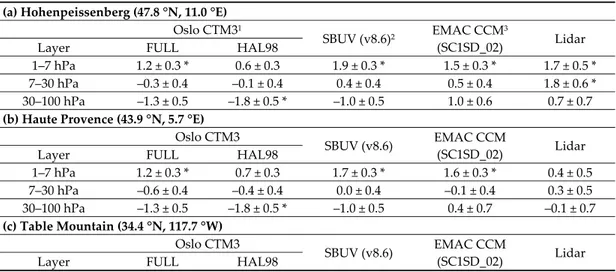
Table 2. Estimated trends (%/decade) in the vertical distribution of ozone for the period of 1998–2016 from observations and model simulations at (a) Hohenpeissenberg, (b) Haute Provence, (c) Table Mountain, (d) Mauna Loa, (e) Lauder and (f) 5 station mean, after removing the seasonal and known natural variability. FULL refers to the main simulation; HAL98 refers to the simulation with fixed halogens at 1998 levels. For lidars, the upper stratospheric layers are confined between 3 and 7 hPa. Asterisks denote statistical significance at the 99% confidence level. (a) Hohenpeissenberg (47.8 °N, 11.0 °E) Oslo CTM31 SBUV (v8.6)2 EMAC CCM 3 (SC1SD_02) Lidar
Layer FULL HAL98
1–7 hPa 1.2 ± 0.3 * 0.6 ± 0.3 1.9 ± 0.3 * 1.5 ± 0.3 * 1.7 ± 0.5 * 7–30 hPa –0.3 ± 0.4 –0.1 ± 0.4 0.4 ± 0.4 0.5 ± 0.4 1.8 ± 0.6 * 30–100 hPa –1.3 ± 0.5 –1.8 ± 0.5 * –1.0 ± 0.5 1.0 ± 0.6 0.7 ± 0.7 (b) Haute Provence (43.9 °N, 5.7 °E) Oslo CTM3 SBUV (v8.6) EMAC CCM (SC1SD_02) Lidar
Layer FULL HAL98
1–7 hPa 1.2 ± 0.3 * 0.7 ± 0.3 1.7 ± 0.3 * 1.6 ± 0.3 * 0.4 ± 0.5 7–30 hPa –0.6 ± 0.4 –0.4 ± 0.4 0.0 ± 0.4 –0.1 ± 0.4 0.3 ± 0.5 30–100 hPa –1.3 ± 0.5 –1.8 ± 0.5 * –1.0 ± 0.5 0.4 ± 0.7 –0.1 ± 0.7 (c) Table Mountain (34.4 °N, 117.7 °W) Oslo CTM3 SBUV (v8.6) EMAC CCM (SC1SD_02) Lidar
1–7 hPa 1.3 ± 0.3 * 0.8 ± 0.3 * 1.6 ± 0.2 * 2.0 ± 0.3 * 0.5 ± 0.8 7–30 hPa –0.9 ± 0.3 * –0.8 ± 0.3 * –0.7 ± 0.3 –0.4 ± 0.3 0.8 ± 0.7 30–100 hPa –3.6 ± 0.6 * –4.0 ± 0.6 * –1.4 ± 0.5 * –0.9 ± 0.8 –2.1 ± 1.6 (d) Mauna Loa (19.5 °N, 155.6 °W) Oslo CTM3 SBUV (v8.6) EMAC CCM (SC1SD_02) Lidar
Layer FULL HAL98
1–7 hPa 0.8 ± 0.2 * 0.4 ± 0.2 1.6 ± 0.2 * 1.5 ± 0.2 * –0.6 ± 0.3 7–30 hPa –0.7 ± 0.3 –0.7 ± 0.3 –0.7 ± 0.3 0.0 ± 0.3 –1.0 ± 0.4 30–100 hPa –4.3 ± 0.8 * –4.7 ± 0.8 * –1.1 ± 0.4 –1.1 ± 0.9 –3.4 ± 0.8 * (e) Lauder (45.0 °S, 169.7 °E) Oslo CTM3 SBUV (v8.6) EMAC CCM (SC1SD_02) Lidar
Layer FULL HAL98
1–7 hPa –0.1 ± 0.3 –0.5 ± 0.3 0.4 ± 0.2 0.5 ± 0.3 0.6 ± 0.5 7–30 hPa –0.4 ± 0.3 –0.3 ± 0.3 0.0 ± 0.4 0.4 ± 0.4 0.7 ± 0.7 30–100 hPa –0.1 ± 0.5 –0.5 ± 0.5 –0.2 ± 0.4 –1.1 ± 0.5 0.5 ± 0.9 (f) 5 Station Mean Oslo CTM3 SBUV (v8.6) EMAC CCM (SC1SD_02) Lidar
Layer FULL HAL98
1–7 hPa 0.9 ± 0.2 * 0.4 ± 0.2 1.4 ± 0.2 * 1.4 ± 0.2 * 0.4 ± 0.2 7–30 hPa –0.6 ± 0.2 * –0.5 ± 0.2 –0.2 ± 0.2 0.1 ± 0.2 0.1 ± 0.3 30–100 hPa –2.1 ± 0.3 * –2.6 ± 0.3 * –1.0 ± 0.3 * –0.3 ± 0.4 –1.3 ± 0.4 * 1Oslo chemistry transport model 3. 2Solar backscatter ultraviolet radiometer (version 8.6). 3EMAC chemistry climate model. Examples of the different trends observed in the upper stratosphere (positive trends) and lower stratosphere (negative trends) are presented in Figure 1. The upper panel shows ozone anomalies over Hohenpeissenberg (HHP), Haute Provence (OHP) and Table Mountain (TMO), and the lower panel shows anomalies at Mauna Loa (MLO) and Lauder (LAU). We remind the reader that natural variability was removed from the data, as described in Section 2.6. As can be seen from Figure 1, the model simulations indicate an increase in ozone in the upper stratosphere, above 7 hPa, and a decrease in the lower stratosphere, between 30 and 100 hPa, in very good agreement with results from the SBUV satellite data. A look into 5° zonal averages from model and satellite data encompassing the stations under study reveals a similar picture too (not shown).
Figure 1. Ozone trends in the upper stratosphere (1–7 hPa), middle stratosphere (7–30 hPa) and lower stratosphere (30–100 hPa), from lidar measurements, SBUV (v8.6) satellite data and Oslo CTM3 simulations over (a) Hohenpeissenberg, (b) Haute Provence and (c) Table Mountain (upper panel), and over (d) Mauna Loa and (e) Lauder (lower panel). Seasonal and natural proxies are removed. For lidars, the upper stratospheric layers are confined between 3 and 7 hPa.
Figure 2 summarizes the comparison of model simulations (Oslo CTM3 and EMAC CCM) with satellite and lidar residuals averaged at all stations under study. The figure shows results for the upper, middle and lower stratosphere for the period of 1998 to 2016. The correlation coefficients (Pearson product‐moment correlation), R, between the four datasets are shown in Table 3 for the five stations’ mean. Results for each station separately are provided in Supplementary Tables S1–S5. Statistical significance of R was determined by using the t‐test formula for the correlation coefficient, with n‐2 degrees of freedom, as by Zerefos et al. [7]. All R are found to be statistically significant at the 99% confidence level or greater. There are higher correlations at some stations, and lower at others, but the general picture of correlations is given in Table 3.
Figure 2. Comparison of CTM ozone simulations (left) and CCM (SC1SD‐base‐02) ozone simulations (right) with SBUV observations and lidar measurements. Shown are ozone anomalies averaged at five lidar stations (HHP–OHP–TMO–MLO–LAU), after removing seasonal and other known natural variability. For lidars, the upper stratospheric layers are confined between 3 and 7 hPa.
Table 3. Statistics of correlations between ozone from Oslo CTM3, EMAC CCM (SC1SD‐base‐02), SBUV (v8.6) and average lidar data anomalies at five stations in the: (a) upper stratosphere (1–7 hPa), (b) middle stratosphere (7–30 hPa) and (c) lower stratosphere (30–100 hPa). Seasonal and other known natural variability were removed from the data. For lidars, the upper stratospheric layers are confined between 3 and 7 hPa.
(a) 1–7 hPa Correlation
Coefficient Intercept (%) Slope Error * t‐Value p‐Value N
CTM3 and SBUV 0.78 0.002 0.700 0.038 18.500 <0.0001 227 CTM3 and Lidar 0.51 –0.040 0.395 0.044 8.912 <0.0001 225 CTM3 and CCM 0.74 0.230 0.715 0.045 15.857 <0.0001 204 CCM and SBUV 0.72 –0.251 0.682 0.047 14.571 <0.0001 203 CCM and Lidar 0.48 –0.207 0.369 0.048 7.688 <0.0001 201 SBUV and Lidar 0.41 –0.038 0.350 0.053 6.640 <0.0001 224 (b) 7–30 hPa CTM3 and SBUV 0.81 0.0007 0.706 0.034 20.560 <0.0001 227 CTM3 and Lidar 0.77 0.026 0.523 0.029 18.064 <0.0001 225 CTM3 and CCM 0.88 0.018 1.008 0.039 26.015 <0.0001 204 CCM and SBUV 0.81 0.016 0.643 0.033 19.707 <0.0001 203 CCM and Lidar 0.77 –0.024 0.459 0.027 16.788 <0.0001 201 SBUV and Lidar 0.71 0.033 0.558 0.037 15.120 <0.0001 224 (c) 30–100 hPa CTM3 and SBUV 0.70 0.008 0.975 0.066 14.859 <0.0001 227 CTM3 and Lidar 0.55 0.179 0.501 0.051 9.834 <0.0001 225 CTM3 and CCM 0.62 –0.155 0.706 0.063 11.129 <0.0001 204
CCM and SBUV 0.67 0.056 0.841 0.066 12.758 <0.0001 203 CCM and Lidar 0.55 0.142 0.450 0.049 9.255 <0.0001 201 SBUV and Lidar 0.62 0.131 0.407 0.035 11.673 <0.0001 224 * Error, t‐value and p‐value refer to slope. We assessed the effect of natural variability on ozone variability. As can be seen from Figure 2, the highest ozone variability is observed in the lower stratosphere, indicative of the strong dynamical influences in that part of the atmosphere related to the QBO, SOLAR, ENSO, AO, tropopause and AOD proxies. The upper stratosphere is much less affected by dynamics, and this fact is evident in both the model and SBUV data. We analyzed the ozone variability in the upper stratosphere, both with and without removing the dynamical proxies. We found that the two estimates do not statistically significantly differ. For example, the 1σ of ozone variability in the upper stratosphere at HHP–OHP–TMO is estimated to be 2.3% after removing the seasonal variability, and 2.2% after removing both the seasonal and dynamical variability related to the QBO, SOLAR, ENSO, AO, tropopause and AOD proxies. In Mauna Loa, ozone variability is estimated to be 1.9% (1σ) after removing the seasonal cycle, and 1.6% after removing both the seasonal and dynamical proxies, while in Lauder, the respective numbers are 2.5% and 2.0%. In all cases, the differences were small, i.e., less than 0.5%. On the other hand, the 1σ of ozone variability is higher in the lower stratosphere than in the upper stratosphere. Indicative values are 3.1% at HHP–OHP–TMO, 3.7% at MLO and 3.5% at LAU after removing the seasonal cycle and dynamical proxies, respectively, compared to 3.9% at HHP–OHP–TMO, 4.4% at MLO and 4.8% at Lauder without removing the dynamical proxies.
Interestingly, the opposite trends seen in the vertical distribution of ozone have resulted in insignificant trends in total ozone after 1997. Reanalysis data from NCEP reveal insignificant trends in tropopause pressures as well. The results are presented in Figure 3, which shows total ozone and tropopause pressure variability at the five stations under study. The respective linear trends are presented in Table 4. Total ozone in the period of 1998–2016 shows small negative statistically insignificant trends.
Figure 3. Time series of total ozone and tropopause pressure anomalies at lidar stations: Hohenpeissenberg and Haute Provence (upper left), Table Mountain (upper right), Mauna Loa (lower left) and Lauder (lower right).
Table 4. Trends (% per decade) in total ozone from SBUV data and tropopause pressure from NCEP reanalysis data for the period 1998–2016, at five lidar stations, after removing variability related to the seasonal cycle and dynamical proxies.
Total Ozone (SBUV v8.6) Tropopause Pressure (NCEP) Trend (% dec−1) t‐Value N Trend (% dec−1) t‐Value N
HHP −0.16 ± 0.33 −0.482 228 −0.06 ± 0.67 −0.089 228 OHP −0.22 ± 0.32 −0.696 228 0.65 ± 0.67 0.964 228 TMO −0.42 ± 0.31 −1.349 228 −0.17 ± 0.79 −0.211 228 MLO −0.26 ± 0.28 −0.954 228 −0.46 ± 0.58 −0.796 228 LAU 0.15 ± 0.30 0.502 228 0.77 ± 0.62 1.247 228 We note here the correlation between the vertical ozone distribution and the total column ozone. The largest R between the layer‐mean ozone and the total column ozone is found in the middle and lower stratosphere, which contain the highest ozone concentrations. We indicate here the contribution of each layer to total ozone in terms of partial ozone columns, based on model simulations, as follows: (a) upper stratosphere (1–7 hPa); average ozone amount 33 DU (10% of total ozone), (b) middle stratosphere (7–30 hPa); average ozone amount 120 DU (36% of total ozone), (c) lower stratosphere (30–100 hPa); average ozone amount 109 DU (33% of total ozone), (d) upper troposphere/lower stratosphere (100–300 hPa); average ozone amount 36 DU (11% of total ozone), and (e) troposphere (300–1000 hPa); average ozone amount 33 DU (10% of total ozone).
The results from the correlation analyses are presented in Table 5, which shows the correlation coefficients, R, between layer‐mean ozone and total ozone, at the stations under study from SBUV satellite data and Oslo CTM3 simulations. The magnitude of correlations gives a measure of the influence of variability of each stratospheric layer to the variability of total ozone. The smaller the correlation, the smaller the influence is. As expected, the upper part of the stratosphere has a small contribution to the short‐term fluctuations of total ozone compared to its middle and lower parts, which contribute the most to total ozone. We remind the reader that the correlations are based on residual data, i.e., data after removing seasonal variability and dynamical proxies, but not the trend component. Long‐term trends contribute to the correlations of Table 5, and therefore the differences between results based on SBUV and CTM total ozone data may be related to differences in their long‐ term trends. Table 5. Correlation coefficients between layer‐mean ozone and total ozone from model (Oslo CTM3) and satellite (SBUV v8.6) data in (a) the upper stratosphere, (b) middle stratosphere and (c) the lower stratosphere at 5 lidar stations, after removing seasonal and known natural variability. Significance at 99.9% is denoted by asterisks. CORRELATION COEFFICIENTS 1998–2016 (a) Upper Stratosphere (1‐7 hPa) and Total Ozone Correlation 1–7 hPa (CTM3) 1–7 hPa (SBUV) Total ozone (SBUV) Total ozone (CTM3) Total ozone (SBUV) Total ozone (CTM3) Hohenpeissenberg 0.24 * 0.28 * 0.31 * 0.31 * Haute Provence 0.22 * 0.23 * 0.30 * 0.28 * Table Mountain 0.34 * 0.19 0.33 * 0.13 Mauna Loa 0.15 0.09 0.14 –0.04 Lauder 0.04 0.04 0.28 * 0.26 * (b) Middle Stratosphere (7–30 hPa) and Total Ozone Correlation
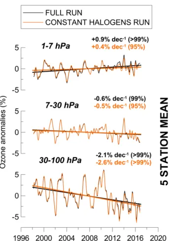
7–30 hPa (CTM3) 7–30 hPa (SBUV) Total ozone (SBUV) Total ozone (CTM3) Total ozone (SBUV) Total ozone (CTM3) Hohenpeissenberg 0.58 * 0.65 * 0.57 * 0.57 * Haute Provence 0.55 * 0.64 * 0.60 * 0.60 * Table Mountain 0.50 * 0.59 * 0.70 * 0.64 * Mauna Loa 0.67 * 0.67 * 0.89 * 0.73 * Lauder 0.65 * 0.66 * 0.75 * 0.69 * (c) Lower Stratosphere (30–100 hPa) and Total Ozone Correlation 30–100 hPa (CTM3) 30–100 hPa (SBUV) Total ozone (SBUV) Total ozone (CTM3) Total ozone (SBUV) Total ozone (CTM3) Hohenpeissenberg 0.81 * 0.87 * 0.90 * 0.75 * Haute Provence 0.76 * 0.86 * 0.90 * 0.72 * Table Mountain 0.73 * 0.88 * 0.92 * 0.77 * Mauna Loa 0.53 * 0.79 * 0.85 * 0.73 * Lauder 0.66 * 0.85 * 0.91 * 0.74 * 3.2. Effect of Chemistry on Ozone Trends With CTM3, we were able to quantify the effect of reducing halogen emissions on the upper‐ and the lower‐stratospheric ozone trends. Simulations with the Oslo CTM3 model (black line) indicate that ozone in the upper stratosphere increased slowly from 1998 to 2016, by about 1% per decade, in agreement with SBUV satellite data. A separate simulation using fixed halogen emissions at 1998 levels (orange line) was performed to evaluate the effect of reducing ozone‐depleting substances on the vertical ozone trends. The results are presented in Figure 4. The trends from the two model simulations (full vs. fixed halogens) were found to differ by 0.5% per decade. This difference is attributed to the reduction of halogen emissions in the atmosphere. In the lower stratosphere, the model reveals statistically significantly negative ozone trends of about −2% per decade. Here, the difference in trends between the two model simulations is also 0.5% per decade; however, we can easily infer that the reduction of halogens after 1997 explains about 55% of the upward trend in the upper stratospheric ozone (1–7 hPa) and about 24% of the trend in the lower stratospheric ozone (30–100 hPa).
Figure 4. Oslo CTM3 simulations of stratospheric ozone. Black line shows trends derived from the main simulation (FULL); orange line shows trends derived from the simulation with constant halogens at 1998 levels. Values in parentheses refer to statistical significance of each trend. Five stations are HHP–OHP–TMO–MLO–LAU. Variability related to the seasonal cycle and dynamical proxies is removed from the data. More analytically, in the case of upper stratospheric ozone, we estimate that the trend would have decreased from 0.9% to 0.4% per decade if halogens had remained constant at 1998 levels after 1998, and in the case of the lower stratospheric ozone, from −2.1% to −2.6% per decade, respectively. We applied a paired t‐test to determine whether the differences between the paired observations (full versus fixed halogen simulations) are significant at the 0.05 level. In both layers, we found that the two means become significantly different after 2001 (upper stratosphere: t = 2.47516, p = 0.01425, N = 180; lower stratosphere: t = 2.19451, p = 0.02949, N = 180). We note that the difference in trends between the two model simulations is almost zero in the middle stratosphere.
3.3. Effect of GHGs on Ozone Trends
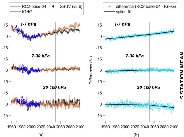
With the CCM simulations, we were able to look into the effect of GHGs increase on long‐term ozone trends. Figure 5 compares two free‐running simulations: a reference simulation with background GHGs mixing ratios (RC2‐base‐04) [21] and the same simulation with fixed GHGs at 1960 levels (SC2‐fGHG‐01) [22]. Blue dots show ozone observations from SBUV (v8.6) satellite data. The right panel shows the differences between the two model simulations (RC2‐base‐04 minus SC2‐ fGHG‐01) as a measure of the effect of global warming on the vertical ozone profiles. The figure refers to the average of five lidar stations. The model reproduces very well the ozone turning point in the upper stratosphere during the 1990s, where the sign of the trends reversed to positive. Good agreement with the satellite observations exists in other layers as well.
(a) (b)
Figure 5. (a) Observed and simulated ozone changes. Model simulations refer to two free‐running CCM simulations, a reference simulation with increasing GHGs emissions according to RCP‐6.0
(RC2‐base‐04) and the same simulation with fixed GHGs emissions at 1960 levels (SC2‐fGHG‐01). (b) Differences (in %) between the two model simulations. The anomalies are deseasonalized data averaged at five stations: HHP–OHP–TMO–MLO–LAU.
In the long‐term, the differences between the two model simulations show a positive trend in the upper stratosphere, no trend in the middle stratosphere and a negative trend in the lower stratosphere, which becomes evident after the 2040s. The upward trend in the upper stratosphere is explained by the fact that increases in GHGs lead to cooling of the upper stratosphere, which slows down temperature‐dependent odd‐oxygen loss processes and increases upper‐stratospheric ozone [22]. On the contrary, lower‐stratospheric ozone is decreasing due to the evolution of GHGs.
In the short‐term, the isolation of the effect of GHGs cannot be identified in the short period from 1998 to 2016, because the signal is too noisy due to internal variability. We conclude that the differences between the two model simulations do not reveal any trend in the period of 1998–2016 due to GHGs. This is in line with the tropopause variability, which shows insignificant trends for the same period (Figure 3). The effect of GHGs on stratospheric ozone trends can be found after 2050, in the RC2‐base‐04 simulation. The mechanism for the change after 2050 is the strengthening in the
meridional (Brewer–Dobson) circulation under enhanced GHGs concentrations. It is most obvious in the tropical region, where we identify stronger upwelling, which can be clearly identified in ozone signatures (i.e., lower ozone values in the tropical lower stratosphere and higher values in the tropical upper troposphere), but also in water vapor and methane, as well as in the temperature field. We note here that the dynamic change can be larger compared to the radiation of GHGs because of feedback mechanisms. Regarding the EMAC model, the complete dynamic feedback of EMAC is in line with other CCM studies. However, it is difficult (so far) to determine (quantitatively) the individual mechanisms regarding the complete dynamic signature, as there are also possible interactions with chemical changes (e.g., feedback with ozone). 3.4. Effect of GHGs on Surface DNA Active UV‐B Irradiance We further studied the impact of GHGs evolution on surface UV‐B irradiance active for DNA damage at the five lidar stations, using CCM simulations (Figure 6). The model simulations are the same as above, i.e., the free‐running simulation with increasing GHGs according to RCP‐6.0 (RC2‐ based‐04) and the sensitivity simulation with constant GHGs at 1960 levels (SC2‐fGHG‐01). The green dots show the deseasonalized DNA‐weighted UV irradiance data from NDACC averaged at Haute Provence, Mauna Loa and Lauder, around local noon, indicating the agreement between the variances in the simulations and the ground‐based measurements. The difference between the two simulations indicates the impact of increased GHGs on DNA active UV‐B irradiance at ground level in the middle‐ and low‐latitude lidar stations. The differences show that DNA active UV‐B irradiance tends to increase by +1.3% per decade after the year 2050, while the respective difference for total ozone does not show any trend after 2050. We find that the trend in UV‐B irradiance is associated with cloud‐cover decrease. The bottom panel shows cloud‐cover variations from the two model simulations for total clouds (1000–200 hPa). The differences between the two simulations (shown on the right) reveal a decreasing trend in total cloud cover of −1.4% per decade after 2050, which is in accordance with the estimated increase in DNA active UV‐B irradiance at ground level. Increased UV‐B irradiance active for DNA damage in the future will have adverse effects on humans and the environment [26].
(a) (b)
Figure 6. (a) Impact of GHGs on total ozone, UV‐B irradiance and clouds based on simulations with increasing and fixed GHGs mixing ratios. RC2‐base‐04 is the simulation with increasing GHGs according to RCP‐6.0; SC2‐fGHG‐01 is the simulation with fixed GHGs emissions at 1960 levels. The anomalies are deseasonalized data averaged at five lidar stations (HHP–OHP–TMO–MLO–LAU). Green dots show deseasonalized DNA‐weighted UV data averaged at OHP, MLO and LAU from the Network for the Detection of Atmospheric Composition Change (NDACC). (b) Difference between the two model simulations.
5. Conclusions
We have analyzed the impact of stratospheric halogen reduction and increase in greenhouse gases on stratospheric ozone changes with the Oslo chemistry transport model and the EMAC chemistry climate model. In addition, we also looked at the effect of increase in greenhouse gases on DNA active UV‐B radiation at ground level. The main results can be summarized as follows: Measurements and CTM simulations with the Oslo model after 1997 for the selected five lidar
stations’ locations show a statistically significant increasing trend in ozone in the upper stratosphere, above 7 hPa, an insignificant decreasing trend in the middle stratosphere, between 7 and 30 hPa, and a significant decreasing trend in the lower stratosphere, between 30 and 100 hPa.
This interchange of positive and negative trends in the vertical ozone profile has resulted in insignificant trends, both in the total ozone column and the tropopause pressure, during the period of study (1998–2016).
As expected from the Oslo CTM3 simulations, the effect of halogen reduction on ozone is maximized at 1–7 hPa at all locations. Comparison between CTM simulations, with fixed and without fixed halogens at 1998 levels, showed that the reduction of halogen‐mixing ratios after 1997 explains about 55% of the observed upward trend in the upper stratospheric ozone (1–7 hPa) (i.e., trend from main simulation: +0.9% per decade, trend from simulation with fixed halogens: +0.4% per decade) and about 24% of the trend in the lower stratospheric ozone (30– 100 hPa) (i.e., trend from main simulation: −2.1% per decade, trend from simulation with fixed halogens: −2.6% per decade).
The effect of GHGs increase on stratospheric profile ozone trends cannot be identified in the short period 1998–2016. As expected from the EMAC CCM calculations, the effect of GHGs becomes evident after the middle of this century. The EMAC CCM projections indicate significant positive trends in the upper stratosphere after the year 2050, insignificant trends in the middle stratosphere and significant negative trends in the lower stratosphere (e.g., [27,28]). Total ozone does not show significant trends after the year 2050 (−0.1% per decade). Solar UV‐B irradiance active for DNA damage at the five lidar stations is estimated to increase on average by +1.3% per decade after the year 2050, associated with a significant decrease in cloud cover of −1.4% per decade due to the evolution of GHGs. In that case, the adverse effects of excessive UV‐B irradiation at these locations are expected to increase due to future global warming. Our estimates regarding the long‐term changes of modeled UV are strongly determined by the cloud behavior in the specific model simulation, and as such, our conclusions about the future behavior of UV are subjected to uncertainties induced by the uncertainties in modeling future clouds. It is beyond the scope of this paper to resolve the issues with clouds in the model. Supplementary Materials: The following are available online at www.mdpi.com/xxx/s1. Table S1: Statistics of correlations between ozone from Oslo CTM3, EMAC CCM (SC1SD‐base‐02), SBUV (v8.6) and Lidar data anomalies in Hohenpeissenberg, in the: (a) upper stratosphere (1‐7 hPa), (b) middle stratosphere (7‐30 hPa) and (c) lower stratosphere (30‐100 hPa). Seasonal and other known natural variability has been removed from the data. For lidars the upper stratospheric layers are confined between 3 and 7 hPa , Table S2: Statistics of correlations between ozone from Oslo CTM3, EMAC CCM (SC1SD‐base‐02), SBUV (v8.6) and Lidar data anomalies in Haute Provence, in the: (a) upper stratosphere (1‐7 hPa), (b) middle stratosphere (7‐30 hPa) and (c) lower stratosphere (30‐100 hPa). Seasonal and other known natural variability has been removed from the data. For lidars the upper stratospheric layers are confined between 3 and 7 hPa, Table S3: Statistics of correlations between ozone from Oslo CTM3, EMAC CCM (SC1SD‐base‐02), SBUV (v8.6) and Lidar data anomalies in Table Mountain, in the: (a) upper stratosphere (1‐7 hPa), (b) middle stratosphere (7‐30 hPa) and (c) lower stratosphere (30‐100 hPa). Seasonal and other known natural variability has been removed from the data. For lidars the upper stratospheric layers are confined between 3 and 7 hPa, Table S4: Statistics of correlations between ozone from Oslo CTM3, EMAC CCM (SC1SD‐base‐02), SBUV (v8.6) and Lidar data anomalies in Mauna Loa, in the: (a) upper stratosphere (1‐7 hPa), (b) middle stratosphere (7‐30 hPa) and (c) lower stratosphere (30‐100 hPa). Seasonal and other known natural variability has been removed from the data. For lidars the upper stratospheric layers are confined between 3 and 7 hPa, Table S5: Statistics of correlations between ozone from Oslo CTM3, EMAC CCM (SC1SD‐base‐02), SBUV (v8.6) and Lidar data anomalies in Lauder, in the: (a) upper stratosphere (1‐7 hPa), (b) middle stratosphere (7‐30 hPa) and (c) lower stratosphere (30‐100 hPa). Seasonal and other known natural variability has been removed from the data. For lidars the upper stratospheric layers are confined between 3 and 7 hPa. Author Contributions: Conceptualization, K.E., J.K. and C.Z.; data curation, S.G.‐B., W.S., C.B., T.L., B.L., R.Q. and D.P.J.S.; formal analysis, K.E. and J.K.; methodology, K.E. and C.Z.; resources, M.D., P.J. and A.S.H; software, J.K. and I.F.; writing—original draft preparation, K.E.; writing—review and editing, C.Z., A.B., I.P., S.G.‐B., P.J., M.D., A.S.H., I.F., T.L. and B.L. All authors have read and agreed to the published version of the manuscript. Funding: We acknowledge support of this work by the project “PANhellenic infrastructure for Atmospheric Composition and climatE change” (MIS 5021516), which is implemented under the action “Reinforcement of the Research and Innovation Infrastructure”, funded by the Operational Programme “Competitiveness,
Entrepreneurship and Innovation” (NSRF 2014‐2020) and co‐financed by Greece and the European Union (European Regional Development Fund).
Acknowledgments: We acknowledge the Long‐term Ozone Trends and Uncertainties in the Stratosphere (LOTUS) activity, supported by SPARC (Stratosphere‐Troposphere Processes And their Role in Climate), WMO and the International Ozone Commission. Also, the Mariolopoulos‐Kanaginis Foundation for the Environmental Sciences. Lidar measurements are performed in the frame of the Network for the Detection of Atmospheric Composition Change (NDACC). Lidar measurements at OHP are funded by the French Centre National de la Recherche Scientifique (CNRS). We acknowledge the work of personnel at the lidar stations. The EMAC simulations have been performed at the German Climate Computing Centre (DKRZ) through support from the Bundesministerium für Bildung und Forschung (BMBF). DKRZ and its scientific steering committee are gratefully acknowledged for providing the HPC and data archiving resources for this consortial project ESCiMo (Earth System Chemistry Integrated Modelling). We acknowledge the SBUV science team for providing the satellite ozone profiles. NIWA UV spectrometer systems, serial numbers UV3 (Mauna Loa, HI) and UV5 (Boulder, CO) in the USA are owned and operated by NOAA/ESRL/Global Monitoring Division, Boulder, CO. They are maintained, calibrated and operated by NOAA. The final data from both of these instruments are quality controlled and produced by NIWA‐Lauder, New Zealand. The data are archived at the NDACC data repository, ftp://ftp.cpc.ncep.noaa.gov/ndacc/station/. We thank NIWA and NOAA for the use of their data in this publication. The study is dedicated to the memory of Prof. Ivar Isaksen.
Conflicts of Interest: The authors declare no conflicts of interest.
References
1. Bais, A.F.; McKenzie, R.L.; Bernhard, G.; Aucamp, P.J.; Ilyas, M.; Madronich, S.; Tourpali, K. Ozone depletion and climate change: Impacts on UV radiation. Photochem. Photobiol. Sci. 2015, 14, 19–52, doi:10.1039/c4pp90032d.
2. Molina, M.J.; Rowland, F.S. Stratospheric sink for chlorofluoromethanes: Chlorine atom catalysed destruction of ozone. Nature 1974, 249, 810–812.
3. WMO. Executive Summary: Scientific Assessment of Ozone Depletion: 2018; Global Ozone Research and Monitoring Project–Report No. 58; World Meteorological Organization: Geneva, Switzerland, 2018; p. 67. 4. den Outer, P.N.; Slaper, H.; Kaurola, J.; Lindfors, A.; Kazantzidis, A.; Bais, A.F.; Feister, U.; Junk, J.; Janouch, M.; Josefsson, W. Reconstructing of erythemal ultraviolet radiation levels in Europe for the past 4 decades. J. Geophys. Res. 2010, 115, D10102, doi:10.1029/2009JD012827. 5. WMO. Scientific Assessment of Ozone Depletion: 2010; Global Ozone Research and Monitoring Project–Report No. 52; World Meteorological Organization: Geneva, Switzerland, 2011; p. 516. 6. Bais, A.F.; Bernhard, G.; McKenzie, R.L.; Aucamp, P.J.; Young, P.J.; Ilyas, M.; Jöckel, P.; Deushi, M. Ozone‐ climate interactions and effects on solar ultraviolet radiation. Photochem. Photobiol. Sci. 2019, 18, 602–640, doi:10.1039/C8PP90059K.
7. Zerefos, C.; Kapsomenakis, J.; Eleftheratos, K.; Tourpali, K.; Petropavlovskikh, I.; Hubert, D.; Godin‐ Beekmann, S.; Steinbrecht, W.; Frith, S.; Sofieva, V.; et al. Representativeness of single lidar stations for zonally averaged ozone profiles, their trends and attribution to proxies. Atmos. Chem. Phys. 2018, 18, 6427– 6440, doi:10.5194/acp‐18‐6427‐2018.
8. Petropavlovskikh, I.; Godin‐Beekmann, S.; Hubert, D.; Damadeo, R.; Hassler, B.; Sofieva, V. (Eds.)
SPARC/IO3C/GAW Report on Long‐Term Ozone Trends and Uncertainties in the Stratosphere; SPARC Report
No. 9, GAW Report No. 241, WCRP‐17/2018; doi:10.17874/f899e57a20b. Available online: www.sparc‐ climate.org/publications/sparc‐reports (accessed on 24 February 2020).
9. Harris, N.R.P.; Hassler, B.; Tummon, F.; Bodeker, G.E.; Hubert, D.; Petropavlovskikh, I.; Steinbrecht, W.; Anderson, J.; Bhartia, P.K.; Boone, C.D.; et al. Past changes in the vertical distribution of ozone–Part 3: Analysis and interpretation of trends. Atmos. Chem. Phys. 2015, 15, 9965–9982, doi:10.5194/acp‐15‐9965‐2015. 10. Ball, W.T.; Alsing, J.; Mortlock, D.J.; Staehelin, J.; Haigh, J.D.; Peter, T.; Tummon, F.; Stübi, R.; Stenke, A.; Anderson, J.; et al. Evidence for a continuous decline in lower stratospheric ozone offsetting ozone layer recovery. Atmos. Chem. Phys. 2018, 18, 1379–1394, doi:10.5194/acp‐18‐1379‐2018. 11. Wargan, K.; Orbe, C.; Pawson, S.; Ziemke, J.R.; Oman, L.D.; Olsen, M.A.; Coy, L.; Knowland, K.E. Recent decline in extratropical lower stratospheric ozone attributed to circulation changes. Geophys. Res. Lett. 2018, 45, 5166–5176, doi:10.1029/2018GL077406.
12. Bais, A.F.; Tourpali, K.; Kazantzidis, A.; Akiyoshi, H.; Bekki, S.; Braesicke, P.; Chipperfield, M.P.; Dameris, M.; Eyring, V.; Garny, H.; et al. Projections of UV radiation changes in the 21st century: Impact of ozone recovery and cloud effects. Atmos. Chem. Phys. 2011, 11, 7533–7545, doi:10.5194/acp‐11‐7533‐2011.
13. Leblanc, T.; Sica, R.J.; van Gijsel, J.A.E.; Godin‐Beekmann, S.; Haefele, A.; Trickl, T.; Payen, G.; Liberti, G. Proposed standardized definitions for vertical resolution and uncertainty in the NDACC lidar ozone and temperature algorithms–Part 2: Ozone DIAL uncertainty budget. Atmos. Meas. Tech. 2016, 9, 4051–4078, doi:10.5194/amt‐9‐4051‐2016.
14. Steinbrecht, W.; Froidevaux, L.; Fuller, R.; Wang, R.; Anderson, J.; Roth, C.; Bourassa, A.; Degenstein, D.; Damadeo, R.; Zawodny, J.; et al. An update on ozone profile trends for the period 2000 to 2016. Atmos.
Chem. Phys. 2017, 17, 10675–10690, doi:10.5194/acp‐17‐10675‐2017.
15. De Mazière, M.; Thompson, A.M.; Kurylo, M.J.; Wild, J.D.; Bernhard, G.; Blumenstock, T.; Braathen, G.O.; Hannigan, J.W.; Lambert, J.‐C.; Leblanc, T.; et al. The Network for the Detection of Atmospheric Composition Change (NDACC): History, status and perspectives. Atmos. Chem. Phys. 2018, 18, 4935–4964, doi:10.5194/acp‐18‐4935‐2018.
16. Godin‐Beekmann, S.; Porteneuve, J.; Garnier, A. Systematic DIAL lidar monitoring of the stratospheric ozone vertical distribution at Observatoire de Haute‐Provence (43.92° N, 5.71° E). J. Environ. Monit. 2003, 5, 57–67, doi:10.1039/B205880D. 17. Kalnay, E.; Kanamitsu, M.; Kistler, R.; Collins, W.; Deaven, D.; Gandin, L.; Iredell, M.; Saha, S.; White, G.; Woollen, J.; et al. The NCEP/NCAR 40‐Year Reanalysis Project. B. Am. Meteor. Soc. 1996, 77, 437–471. 18. Søvde, O.A.; Prather, M.J.; Isaksen, I.S.A.; Berntsen, T.K.; Stordal, F.; Zhu, X.; Holmes, C.D.; Hsu, J. The chemical transport model Oslo CTM3. Geosci. Model Dev. 2012, 5, 1441–1469, doi:10.5194/gmd‐5‐1441‐2012. 19. Prather, M.J. Photolysis rates in correlated overlapping cloud fields: Cloud‐J 7.3c. Geosci. Model Dev. 2015, 8, 2587–2595, doi:10.5194/gmd‐8‐2587‐2015.
20. Sander, S.P.; Abbatt, J.; Barker, J.R.; Burkholder, J.B.; Friedl, R.R.; Golden, D.M.; Huie, R.E.; Kolb, C.E.; Kurylo, M.J.; Moortgat, G.K.; et al. Chemical Kinetics and Photochemical Data for Use in Atmospheric Studies; Evaluation No. 17; JPL Publication: Jet Propulsion Laboratory, Pasadena, CA, USA, 2011. Available online: http://jpldataeval.jpl.nasa.gov (accessed on 12 September 2018).
21. Jöckel, P.; Tost, H.; Pozzer, A.; Kunze, M.; Kirner, O.; Brenninkmeijer, C.A.M.; Brinkop, S.; Cai, D.S.; Dyroff, C.; Eckstein, J.; et al. Earth System Chemistry integrated Modelling (ESCiMo) with the Modular Earth Submodel System (MESSy) version 2.51. Geosci. Model Dev. 2016, 9, 1153–1200, doi:10.5194/gmd‐9‐1153‐ 2016. 22. Dhomse, S.S.; Kinnison, D.; Chipperfield, M.P.; Salawitch, R.J.; Cionni, I.; Hegglin, M.I.; Abraham, N.L.; Akiyoshi, H.; Archibald, A.T.; Bednarz, E.M.; et al. Estimates of ozone return dates from Chemistry‐Climate Model Initiative simulations. Atmos. Chem. Phys. 2018, 18, 8409–8438, doi:10.5194/acp‐18‐8409‐2018. 23. Sander, R.; Jöckel, P.; Kirner, O.; Kunert, A.T.; Landgraf, J.; Pozzer, A. The photolysis module JVAL‐14, compatible with the MESSy standard, and the JVal PreProcessor (JVPP). Geosci. Model Dev. 2014, 7, 2653– 2662, doi:10.5194/gmd‐7‐2653‐2014. 24. Brühl, C.; Crutzen, P.J. On the disproportionate role of tropospheric ozone as a filter against solar UV‐B radiation. Geophys. Res. Lett. 1989, 16, 703–706. 25. McKenzie, R.; Bernhard, G.; Liley, B.; Disterhoft, P.; Rhodes, S.; Bais, A.; Morgenstern, O.; Newman, P.; Oman, L.; Brogniez, C.; et al. Success of Montreal Protocol Demonstrated by Comparing HighQuality UV Measurements with “World Avoided” Calculations from Two Chemistry‐Climate Models. Sci. Rep. 2019, 9, 12332, doi:10.1038/s41598‐019‐48625‐z. 26. Lucas, R.M.; Yazar, S.; Young, A.R.; Norval, M.; de Gruijl, F.R.; Takizawa, Y.; Rhodes, L.E.; Sinclair, C.A.; Neale, R.E. Human health in relation to exposure to solar ultraviolet radiation under changing stratospheric ozone and climate. Photochem. Photobiol. Sci. 2019, 18, 641–680, doi:10.1039/C8PP90060D.
27. Braesicke, P.; Neu, J.; Fioletov, V.; Godin‐Beekmann, S.; Hubert, D.; Petropavlovskikh, I.; Shiotani, M.; Sinnhuber, B.‐M. Update on Global Ozone: Past, Present, and Future. In Scientific Assessment of Ozone
Depletion: 2018; Global Ozone Research and Monitoring Project–Report No. 58; World Meteorological
Organization: Geneva, Switzerland, 2018; Chapter 3.
28. Langematz, U.; Tully, M.; Calvo, N.; Dameris, M.; de Laat, A.T.J.; Klekociuk, A.; Müller, R.; Young, P. Polar Stratospheric Ozone: Past, Present, and Future. In Scientific Assessment of Ozone Depletion: 2018; Global Ozone Research and Monitoring Project–Report No. 58; World Meteorological Organization: Geneva, Switzerland, 2018; Chapter 4. © 2020 by the authors. Licensee MDPI, Basel, Switzerland. This article is an open access article distributed under the terms and conditions of the Creative Commons Attribution (CC BY) license (http://creativecommons.org/licenses/by/4.0/).