HAL Id: halshs-00348810
https://halshs.archives-ouvertes.fr/halshs-00348810
Submitted on 22 Dec 2008
HAL is a multi-disciplinary open access
archive for the deposit and dissemination of
sci-entific research documents, whether they are
pub-L’archive ouverte pluridisciplinaire HAL, est
destinée au dépôt et à la diffusion de documents
scientifiques de niveau recherche, publiés ou non,
Risk Perception, Risk Attitude and Decision : a
Rank-Dependent Approach
Michèle Cohen
To cite this version:
Michèle Cohen. Risk Perception, Risk Attitude and Decision : a Rank-Dependent Approach. 2008.
�halshs-00348810�
Documents de Travail du
Centre d’Economie de la Sorbonne
Risk Perception, Risk Attitude and Decision :
a Rank-Dependent Approach
Michèle C
OHEN2008.84
Risk Perception, Risk Attitude and Decision :
a Rank-Dependent Approach
Michèle Cohen
Paris School of Economics and
CES -University Paris I, Panthéon-Sorbonne
December 3, 2008
Résumé
Le modèle classique d’espérance d’utilité dans le risque a été critiqué aussi bien d’un point de vue expérimental (Paradoxe d’Allais) que pour son manque de pouvoir explicatif. The modèle Rank-Dependent Expected Utility (RDU) (Quiggin 1982) tente de répondre à certaines de ces critiques. Le décideur est caractérisé par deux fonctions : une fonction d’utilité qui mesure la satisfaction des résultats dans le certain et une fonction de transformation des probabilités qui mesure le poids subjectif des probabilités. Nous montrons, dans ce papier, que le modèle RDU permet des comportements plus diversi…és : il est cohérent avec le paradoxe d’Allais ; le décideur peut ne pas aimer le risque (préférer à toute décision son espérance) sans nécessairement éviter tout accroissement de risque (à espérance constante) ; un décideur peut avoir une utilité marginale décroissante tout en ayant du goût « faible » pour le risque ; deux décideurs ayant la même fonction d’utilité peuvent avoir des comportements di¤érents s’ils ont des fonctions de transformation des probabilités di¤érentes ; de plus, le même décideur peut avoir des croyances subjectives sur les événements qui dépendent du contexte.
Mots clé: décision dans le risque, perception des risques, aversion pour le risque, paradoxe d’Allais, modèle Rank-Dependent Expected Utility.
Abstract
The classical expected utility model of decision under risk (von Neumann-Morgenstern, 1944) has been criticized from an experimental point of view (Al-lais’ paradox) as well as for its restrictive lack of explanatory power. The Rank-Dependent Expected Utility model (RDU) model (Quiggin, 1982) attempts to answer some of these criticisms. The decision maker is characterized by two functions: a utility function on consequences measuring preferences over sure outcomes and a probability weighting function measuring the subjective weight-ing of probabilities. As we show and illustrate in this paper, this model allows for more diversi…ed types of behavior: it is consistent with the behavior revealed by the Allais paradox; the decision maker could dislike risk (prefer to any lottery its expectation) without necessarily avoiding any increase in risk; diminishing marginal utility may coexists with "weak" risk seeking attitudes; decision mak-ers with the same utility function may di¤er in their choices between lotter-ies when they have di¤erent probability weighting functions; furthermore, the same decision maker may have di¤erent, context-dependent, subjective beliefs on events.
Key words: Decision under risk, risk perception, risk aversion, Allais para-dox, Rank-Dependent Expected Utility model.
*Classi…cation-JEL : D81
Acknowledgement
I am most grateful to André de Palma, Johanna Etner, Meglena Jeleva, Isaac Meilijson, Benoit Menoni, Nicolas Roux and two anonymous referees for very helpful suggestions and comments.
1 Introduction
The Expected Utility (EU) model, introduced in the seminal work of von Neu-mann and Morgenstern (1944) is the classical model of decision under risk. The well known Allais paradox (Allais 1953) provides experimental evidence that the observed behavior of a majority of DMs is in contradiction with the EU model. Further criticisms of the EU model concerns its lack of explanatory power: (1) The same function u characterizes two distinct attitudes: attitude to-wards risk and attitude toto-wards wealth (shape of the marginal utility) that have no a-priori reason to be identi…ed with each other ; so, if a DM, adhering to the EU model, has a diminishing marginal utility (i.e., u is concave), then he must be risk averse.
(2) Theoretically, it could be possible that a DM avoids risk whenever pos-sible, but faced with two risky situations, chooses the riskier one with the hope of a higher gain: Weak Risk Aversion (preferring to any random variable its expected value) needs not imply Strong Risk Aversion (aversion to mean pre-serving increases in risk). Under EU, Weak Risk Aversion forces u to be concave, and this, in turn, implies Strong Risk Aversion.
(3) Experimental …ndings (Slovic 1987) show that the probability of the same event can be perceived di¤erently, depending on subjective properties of the DM and, for the same DM, on subjective characteristics of the decision problem encountered. These di¤erent ways of weighting probabilities cannot be taken into account in the EU framework.
(4) There are observed economic behaviors that can not be explained in the framework of the EU model as, for instance, the behavior of a policy holder, asking for complete insurance even though the premium is loaded.
The Rank-Dependent Expected Utility (RDU) model (Quiggin 1982, Yaari 1987, …rst version 1982) has been built, in part, as an attempt to answer to some of these criticisms.
The purpose of this paper is to illustrate how does the RDU model, which is more ‡exible than the EU model, accommodate the diversity of behaviors mentioned above. The paper is organized as follows: Section 2 introduces the general framework of a decision making problem under uncertainty and estab-lishes some convenient notations. Section 3 introduces di¤erent concepts of increase in risk and risk aversion (risk seeking being the dual concept), as inde-pendently as possible of the exact model of decision under risk adopted. The treatment of these concepts under EU presented in Section 4, unduly restrictive, is contrasted in Section 5 by the ‡exibility of the RDU model in di¤erentiating between the various concepts of risk aversion.
2 The decision problem under uncertainty:
gen-eral presentation
Most of our decisions concerning, for instance, employment, investment, insur-ance, portfolio choice, health, transportation, quality of life or quality of our environment... are taken in an uncertain situation. We have to choose a deci-sion without knowing its consequences with certainty because they depend on events that may or may not occur. Thus, the study of decision making needs, …rst of all, an appropriate formalization of decision problems under uncertainty. We have …rst to de…ne formally the set of decisions. We take as primitive a set of states of nature, S, representing the set of all elementary events that can occur, and a set C of all possible consequences for this problem. A decision is then a mapping from the set of states of nature S to the set of consequences C. The consequence set is speci…c to a given decision problem: it can contain only monetary outcomes, but its elements can also correspond to consumption levels, employment levels, qualities of health or qualities of life, transportation times....The set of states of nature has to be described su¢ciently precisely for the given decision problem and …nally, the available information on events has to be identi…ed in order to construct a "belief" on the events.
2.1 Typology of situations of uncertainty
In decision theory, we make a distinction between di¤erent types of information on events, subsets of S, set of states of nature.
The term "risk " is reserved to situations in which all events of S have "ob-jective" probabilities with which the DM agrees (Knight, 1921). This is typically the case in games of chance, such as card games, roulette...; risk also encom-passes all situations in which reliable statistical data are available: risk of car accident according to the type of driver and vehicle, risk of heart attack for a 55 year old person with high blood pressure, risk of ‡ood. . . .
All the other situations without such (probabilistic) information are called situations of uncertainty. Let us just mention di¤erent kinds of uncertainty :
(i) Imprecise risk: the probability of each event is only known to belong to an interval ; (ii) Complete uncertainty : we know all the elements of the set S but no further information on the events ; (iii) Radical uncertainty: the entire set of states of nature is not completely identi…ed and the unknown states are denoted "unforeseen contingencies"1.
In Bayesian decision theory, the Decision Maker acts under any type of uncer-tainty as if he could always summarize the unceruncer-tainty by a subjective probabil-ity and thus uses a model of decision under risk. However, it has been observed experimentally (Ellsberg, 1961) that individuals dislike ambiguity, meaning that
1Even though we will not study here these situations, let us just notice some examples that
occured these last decades : Aids, Contamined blood, mad cow, 9/11, GMO, risks of cancer linked with the cellular phones ...., cases where the possibility of these events has not even been anticitaped.
they prefer a situation of risk to an uncertain one, and such a behavior is in-compatible with Bayesian theory.
Nevertheless, in order to improve our understanding of behavior in uncertain situations, we will focus, in this paper, to a situation of risk.
From now on, we will assume that the probability distribution on the set S is given; we are thus dealing with a problem of decision under risk.
2.2 Given probability and perceived risk
It is well established now, since Slovic (1987), that there exists a di¤erence between "given" probabilities (issues from frequencies or probabilistic calculus) and "perceived" probabilities that a DM uses to evaluate his decisions.
Risk perception appears to depend not only on the DM’s characteristics but also, for the same DM, on the decision problem he is facing and on the context in which the decisions are taken.
In the following, we give some examples on DM’s and decision problem’s characteristics that have been pointed out as relevant for risk perception (see for example Slovic, 1987 ; Weber, 1997 ; Weber, Blais and Betz, 2002). Moreover the DM’ characteristics like gender, culture, level of education, level of knowl-edge, di¤erences between experts and non-experts, risk perception may depend on decision problem’s or context’s characteristics. For the same probability (Slovic, 1987), the "perceived" risk (considered here as danger) can depends on: (i) whether the danger is controlled or not (chosen vs undergone danger like, for example, in a car’s travel, driver vs passenger); (ii) whether there is equity or not about the consequences (nuclear wastes in a neighborhood where inhab-itants have or not taken advantage of the nuclear power); (iii) whether there is catastrophic potential or not (car accident vs aircraft accident); (iv) whether there is reversibility of the danger or not (ski accident vs nuclear accident); (v) whether there is knowledge (or familiarity) of the danger or not (household accident vs nuclear accident);
Another factor, that may be more important than all those mentioned be-fore, can in‡uence the perceived probability: the link between beliefs and con-sequences. A DM does not treat a given probability the same way when corre-sponding to a "good" consequence or correcorre-sponding to a "bad" consequence ; the perception may also depend on the reference point (see for instance Kahneman and Tversky, 1979).
How to deal with the di¤erences between given risk and perceived risk ?
Knowing that di¤erent decision makers with the same given information construct di¤erent subjective beliefs and di¤erent preferences, it is important, from an individual point of view as well as from a public policy (or an insurance company) point of view, to know how each DM constructs his preferences, using his risk perception and his attitude towards risk.
Knowing that, in the classical Expected Utility model, it is not possible to discriminate, for the same given probability, between di¤erent risk perceptions,
how can we …ll the gap between all these experimental …ndings and the classical model? How can we take into account such di¤erences in risk perception?
We will try to prove that RDU model is a partial answer to these questions and we will show that, for a RDU Decision Maker, the probability weighting function ' can be a way of linking the DM perceived probability to conse-quences, and that all the other factors in‡uencing the perception of risk can be modelled as additional parameters to the ' function.
2.3 Formalization and Notations
A general problem of decision making under uncertainty is formalized by intro-ducing a set S called set of states of nature, identifying events to subsets of S; forming a ¾-algebra A. If we denote by C a set of consequences, a decision is then a mapping from (S; A) to C. We denote by X the set of such mappings (set of decisions).
For a given decision problem, each DM has a preference relation denoted % on X which is assumed to be a weak order (i.e. a re‡exive, transitive and complete relation); the strict preference is denoted  and the indi¤erence ». This relation on X induces (by the way of constant mappings) a preference relation on C, also denoted by %.
The purpose is to represent the DM’s preferences (X; %) by a real-valued utility function, (i.e. a mapping V from X toR such that: X % Y () V (X) ¸ V (Y )).
Since we are under risk, the set (S; A) is equipped with a probability measure P. Any decision X of X is then a random variable2 and has then a probability
distribution denoted PX; Let FX denote the cumulative distribution function
of PX : FX(x) = PfX · xg and E (X) its expected value.
Under the classical assumption that two random variables with the same probability distribution are indi¤erent, the preference relation % on X induces, on the set of probability distributions on C, denoted L, a preference relation also denoted %. This assumption means, in fact, that the preference relation depends only on the consequences and their probabilities.
We also identify the consequence c 2 C with the Dirac function ±c at c
(±c2 L) and we equivalently denote: ±c% PX or c % PX or c% X.
Here, for the sake of simplicity, we assume that C is a closed and bounded interval of R. In some sections, we limit our study to the set L0 of …nite
probability distributions on C ; generic element of L0 will be denoted PX =
(x1; p1; :::; xn; pn) where the consequences are always ranked with increasing
or-der : x1· ::: · xn, with pi¸ 0 andPpi= 1.
Moreover, we de…ne F¡1from (0; 1] intoR by F¡1(p) = inffz 2 RjF (z) ¸ pg,
the highest gain among the least favorable p% of the outcomes.
3 Attitude towards risk
Risk aversion has two aspects: preference for certainty when it is possible to avoid any risk, and preference for reduction of risk when it is impossible to completely eliminate risk.
Thus, the …rst notion of risk aversion corresponds to a propensity to choose, when possible, to avoid risk, or more precisely, to always prefer to any random variable X the certainty of its expected value E(X ). However, when it is not possible to completely eliminate the risk, this notion is not su¢cient to compare the riskiness of two random variables.
Aversion to increase in risk is more delicate to de…ne because many di¤erent concepts of increase in risk that can be proposed. To any type of increase in risk will be associated a speci…c de…nition of risk aversion (corresponding to aversion to this type of increase in risk).
Let us …rst give two notions of increase in risk.
3.1 De…nition and properties of di¤erent notions of
in-crease in risk
In this section, to de…ne a partial order on random variables (namely, Y is an increase in risk of X), and focus our attention to the riskiness of these random variables, we will only compare random variables with the same mean.
For X and Y with the same mean, Y is a general mean preserving increase in risk or Mean Preserving Spread (MPS) of X ifRt
¡1FY(x)dx¸
Rt
¡1FX(x)dx
for all t 2 R.
This classical notion, special case, for equal means, of second order stochastic dominance, was introduced in economics by Rothschild and Stiglitz (1970). A more intuitive characterization is that the more risky Y is obtained by adding a noise (random variable independent of X and with 0 mean) to X.
Rothschild and Stiglitz themselves (1971) showed that there exist many eco-nomic situations where their notion of increase in risk does not seem to …t well to the problem. For example, let us assume Y M P S X and two EU decision makers such that D2 is more risk averse than D1 and D1 is ready to pay c to exchange Y for the less risky X : in a very counter-intuitive way, it can be the case that D2, more risk averse than D1, is ready to pay less than c for the same exchange.
Some of these counter-intuitive examples gave rise to other notions of in-crease in risk (see Jewitt 1989 ; Lansberger and Meilijson, 1994 ; Chateauneuf and alii, 2004). In particular, Quiggin (1992) de…ned a more demanding no-tion of increase in risk, more …tted with many economic problems3, where, for
instance, the above counter-intuitive result can no more be possible :
For X and Y with the same mean, Y is a Monotone Mean Preserving Spread (MMPS) with respect to X if F¡1
Y (q)¡ FY¡1(p)¸ FX¡1(q)¡ FX¡1(p) for all
0 < p < q < 1.
The interpretation of this formula is that all the interquantile intervals are shorter for X than for Y4. With this interpretation, no one could deny that Y
is more risky than X (being more dispersed everywhere). The following table shows examples of these di¤erent increases (reductions) of risk.
Table 1 : Examples of di¤erent concepts of increase (reduction) in risk Pr oba 1=5 1=5 1=5 1=5 1=5 Y ¡2000 ¡1000 0 1000 2000 Initial risk X1 ¡2000 0 0 0 2000 Rothschild¡ Stiglitz reduction of risk X2 ¡1250 ¡500 0 500 1250 M onotone reduction of risk
X3 0 0 0 0 0 reduction of riskComplete
It can easily be proved that Y M P S X1and Y MP S X2but only Y MMP S X2:
Let us try to add more justi…cation of this new concept of monotone in-crease in risk: looking at the probability distribution in Table 1 as an income distribution, then, exchanging Y for X2 can always be viewed as a reduction of
inequalities, whereas exchanging Y for X1, can no more be viewed as a
reduc-tion of inequalities and at least for the poorest one, could even be viewed as an increase in inequalities.
Remark 1 Let us just mention that there exist also other de…nitions of increas-ing risk (reducincreas-ing risk) that do not treat symmetrically good and bad results like the concepts of downside risk (see C Menezes and alii, 1980) or left monotone increase in risk (Jewitt, 1989 ; Landsberger and Meilijson, 1994 ; Chateauneuf and alii, 2004).
3.2 Model-free concepts of risk aversion, risk seeking
For a DM with a preference relation % on X; we can now give three model-free concepts of risk aversion and their precise de…nitions.
² A DM has Weak Risk Aversion (WRA) if, for any random variable X of X, he prefers to the random variable X, its expected value E(X) with
certainty: 8X 2 X; E(X) % X ; has Weak Risk-Seeking(WRS) if 8X 2 X; X% E(X) ; is risk-neutral if 8X 2 X; X » E(X ).
Each other concept of risk aversion will now be de…ned as aversion to a particular concept of increase in risk.
² A DM has Strong Risk Aversion (SRA), if, for any pair of random vari-ables X; Y in X with Y being a Mean Preserving Spread of X, he always prefers X to Y : 8X; Y 2 X; Y MP S X =) X % Y ; has Strong Risk-Seeking(SRS) if 8X; Y 2 X; Y MPS X =) Y % X ; is risk-neutral if X» Y .
Intuitively, these two notions capture distinct behaviors: a DM may want to avoid completely risk when possible, but when he cannot do so and has to choose between two situations where he cannot avoid risk, he could choose the riskier one, hoping to get the best consequences.
The third concept is based on aversion to monotone increases in risk : ² A DM has Monotone Risk Aversion (MRA), if, for any pair of random
variables X; Y of X with Y Monotone Mean Preserving Spread (MPS) of X, he always prefers X to Y : 8X; Y 2 X; Y M MPS X =) X % Y ; has Monotone Risk-Seeking (MRS) if 8X;Y 2 X; Y MMP S X =) Y % X ; is risk-neutral if X » Y .
The notion of Weak Risk Aversion was de…ned by Arrow and Pratt (1961). If we compare Weak Risk Aversion and Strong Risk Aversion, we can notice that, since for any X, X is a mean preserving spread of E(X), Strong Risk Aversion implies Weak Risk Aversion. The reciprocal implication is not true in general.
More generally, it can be proved that5:
Strong Risk Aversion =) Monotone Risk Aversion =) W eak Risk Aversion
while the reciprocal assertions are not necessarily true.
4 The Expected Utility Model
4.1 General presentation
The classical normative model (due to von Neumann and Morgenstern, 1944), the Expected Utility (EU) model, is based on simple and appealing axioms and
has important properties6. Let us recall brie‡y the value function representing
the preferences in this axiomatic model.
For a decision PX = (x1; p1; :::; xn; pn), preferences can be represented by a
functional U; such that : U (PX) = EP(u(X)) =
Pn
i=1piu(xi) where u is a mapping from C to R
de…ned by u(x) = U(±x) strictly increasing and unique up to an a¢ne increasing
weighting.
In this formula, the functional U is linear in probabilities. This formula can also be written as:
U (PX) = u(x1)+::+( j=nP j= i+ 1
pj)[u(xi+1)¡u(xi)] +¢ ¢ ¢+(pn)[u(xn)¡u(xn¡1)] (1)
The best decision is the one maximizing this Expected Utility. Let us notice that a DM, who behaves in accordance to the EU model, is completely charac-terized by this unique function u ; thus, EU is a very parsimonious model.
4.2 Characterization of di¤erent notions of risk aversion
in the EU model
In this model, it has been proved, since 1970, by Rothschild and Stiglitz that: (i) Weak Risk Aversion is equivalent to the concavity of u;
(ii) Strong Risk Aversion is equivalent to the concavity of u: Thus, these two results imply that, in the framework of EU model,
Strong Risk Av:() Monotone Risk Av: () W eak Risk Av: () Concavity of u
This means that, in the EU model, as soon as the DM has Weak Risk Aversion, he has necessarily Monotone Risk Aversion and Strong Risk Aversion. Thus, the EU model cannot take into account some diversi…ed behaviors like having Weak but not Strong Risk Aversion.
4.3 Discussion on the EU model
4.3.1 Advantages
This classical model has many nice properties. The EU model has axiomatic foundations; the axioms are simple and appealing. Moreover, Bayes rule pro-vides an intuitive updating rule and the linearity in probabilities guarantees dynamic consistency which allows the treatment of decision trees by dynamic programming.
Despite its numerous advantages, the EU model has been questioned for not taking into account, in many situations, the DM’s observed behavior.
6For an axiomatic presentation of the model, and all its properties, see for instance Kreps
4.3.2 Drawbacks
Allais’ paradox From an experimental point of view, the well-known Allais’ paradox has pointed out, since 1953, that real behavior of a ma jority of DMs is in contradiction with the EU model. Let us …rst recall this Allais paradox (Allais, 1953) that gave rise to the new models of behavior under risk. In fact, we expose an example from Kahneman and Tversky (1979) similar to Allais paradox. Subjects are requested to express their preferences …rst between these two prospects:
² A: winning $3; 000 with probability 1 or B : winning $4; 000 with proba-bility 0:8
and then, independently, between the two prospects :
² C : winning $3; 000 with probability 0:25 or D : winning $4; 000 with probability 0:20.
Typical preferences are A Â B and D Â C: Such preferences are in contradic-tion with the EU model: indeed, setting, without lack of generality, u(4000) = 1 and u(0) = 0 and u(3000) = ®, 0 < ® < 1; A Â B implies, in the EU model, ® > 0:80 whereas DÂ C implies 0:25® < 0:20, a contradiction.
This type of experiment has been conducted many times with heterogeneous samples, in di¤erent countries and each time, about 2=3 of the subjects gave the choices A and D:
Other drawbacks There are more criticisms concerning the lack of explana-tory power of the EU model.
(1) As we already mention in the introduction, the EU model also raised a theoretical di¢culty, namely, the interpretation of the function u (Bernoulli’s utility function) characterizing the decision-maker’s behavior. Indeed, as pointed out by Allais, the function u has a double role of expressing the DM’s attitude with respect to risk (concavity of u implying risk aversion) and the DM’s val-uation di¤erences under certainty (concavity of u implying then diminishing marginal utility of wealth), so that, for instance, it is impossible to explain, in this model, the behavior of a DM having at the same time a diminishing marginal utility for certain wealth and a risk seeking attitude.
(2) In the same way, the attitude of a DM having Weak Risk Aversion with-out having automatically Strong Risk Aversion is not allowed in the framework of EU model.
(3) As mentioned in the introduction, the probability of the same event can be perceived di¤erently, depending on many subjective characteristics of the decision problem and also many sub jective characteristics of the DM. These di¤erent ways of "weighting" probabilities, again, cannot be taken into account in the EU framework where the DM is always supposed to use the same "given"
There are many economic illustrations of the rigidity of the model as ex-plained, for instance, in Rothschild and Stiglitz (1971). As we already mention in the introduction, since, in the EU mo del, it is never optimal to take a com-plete insurance coverage when the premium is loaded, this EU model cannot explain why many policy holders buy complete insurance coverage, knowing that, in insurance companies, the premium is always loaded7.
For these reasons, even if the EU model has the advantage to be parsimonious (with only one function u to assess), since many observed economic behaviors cannot be explained in the framework of this model, we will present, in the next section, the Rank-Dependent Expected Utility (RDU) model (Quiggin, 1982), a more general model, less parsimonious but more explanatory, built, in part, as an attempt to answer to some of the criticisms of the EU model.
5 The Rank Dependent Expected Utility model
5.1 General presentation
The Rank Dependent Expected Utility (RDU) model is due to Quiggin (1982) under the denomination of Anticipated Utility. Variants of this model are due to Yaari (1987, …rst version, 1982), and Allais (1988). More general axiomati-zations can be found in Wakker (1994), Chateauneuf (1997).
A DM behaves in accordance with the Rank-Dependent Expected Utility (RDU) model if the DM’s choices between decisions are characterized by two func-tions u and ':
(i) a continuous, increasing utility function u: C ! R (that plays the role of utility on certainty ) and
(ii) an increasing probability weighting function ' : [0; 1] ! [0; 1] that satis…es '(0) = 0; '(1) = 1.
Such a DM prefers the decision X to the decision Y if and only if V (X)¸ V (Y ), where the functional V is given by :
V (X) = u(x1)+::+'( j=nP
j=i+1pj)[u(xi+1)¡u(xi)]+¢ ¢ ¢+'(pn)[u(xn)¡u(xn¡1)]
(2) V (X) happens to be a Choquet integral (Choquet 1953).
We can interpret u as the satisfaction of the consequences and ' as the way the DM transforms the decumulative probabilities.
Let us give an interpretation of this valuation. The DM takes for sure the utility of the worst outcome u(x1) and weights the additional possible increases
7Let us mention another example: In the theory of portfolio choice, the observed behavior
of a DM, putting all his wealth in the riskless asset, even though the expected value of the risky asset’s rate is greater than the safe rate, is incompatible with the EU model.
of utility [u(xi)¡u(xi¡1)] by his personal weighting '( j=nP j=i+1 pj) of the probability j=nP j=i+1 pj of getting at least xi.
According to this interpretation of the formula, if the DM is such that ' (p) · p for all p in [0; 1]; comparing the formula giving respectively EU and RDU functionals, it means that this DM underweights all the additional utilities of gains. Thus, we give the following de…nitions.
² A RDU DM with a function ' such that 8p in [0; 1]; ' (p) · p; is called a pessimist under risk.
² A RDU DM with a function ' such that 8p in [0; 1]; ' (p) ¸ p; is called an optimist under risk.
Let us …nally notice that, if the weighting function ' is the identity function '(p) ´ p, formula 1 and 2 are then identical, V (X) reduces to the expected utility of the random variable.
5.2 Evaluating a simple decision (EU vs RDU)
A very simple example can be used to show the role of a probability weighting function '. Let X be a simple decision giving consequence x1 with probability
1¡ p and x2with probability p.
Valuation of X in a EU model: U (X) = (1 ¡ p)u(x1) + pu(x2)
Valuation of X in a RDU model: ½
RDU (X) = [1¡ '(p)]u(x1) + '(p)u(x2) if x1· x2
RDU(X ) = '(1¡ p)u(x1) + [1¡ '(1 ¡ p)]u(x2); if x1¸ x2
If ' is di¤erent from identity, the DM will not evaluate the same event with the same weight depending on whether the event is favorable or unfavorable. If the DM is pessimistic under risk, he always underweights the probability of the best outcome and overweights the probability of the worse outcome.
Numerical example: S = fs1; s2g. S has two elements with respective
probabilities 2=10 and 8=10.
The following table gives, in the two …rst columns, directly the utilities of the outcomes for the two decisions X and Y according to which state occur, and in the three next columns, the valuation of these two decisions in EU and in two types of RDU models.
2=10 8=10 E U RDU (pess) RDU (opt) '(p) = p2 '(p) = pp
X ¡1000 0 ¡200 ¡360 ¡105:6
² Valuation in EU: U(X) = ¡200 ; U(Y ) = 200
² Valuation in RDU with '(p) = p2;for p in[0; 1]; revealing pessimism under
risk since 0 · p2· p · 1.
We evaluate '(0:20) = 0:04; 1 ¡ '(0:20) = 0:96; '(0:80) = 0:64;1¡ '(0:80) = 0:36; For such a pessimist DM, when 0 corresponds to an unfavorable event, its probability is over-estimated whereas the same probability is under-estimated when 0 corresponds to a favorable event.
Since ¡1000 < 0, RDU (X) = ¡1000¤0:36+ 0¤0:96 = ¡360; since 0 < 1000; RDU(Y ) = 0¤ 0:96 + 1000 ¤ 0:04 = 40:
² The last column of the table corresponds to the values of a RDU DM with '(p) = pp, for p in[0; 1]; revealing optimism under risk, since 0 · p · pp· 1:
The probability weighting function ' depends thus on the DM. Moreover, if we want to model the fact that risk perception depends also on the context in which the decisions are taken, for a DM having a utility function u, his probability weighting function ' could depend on a parameter 's(:) where s
characterizes the context (section 5.5.2.).
5.3 Characterization of di¤erent notions of risk aversion
in the RDU model
The di¤erent concepts of risk aversion, while equivalent in EU theory, have di¤erent characterizations in the RDU model. However, there is a common necessary condition for the three di¤erent concepts of Risk Aversion:
Pessimism under risk : '(p) · p; for p in[0; 1]: 5.3.1 Strong Risk Aversion/Risk-Seeking
Chew, Karni and Safra (1987) found an appealing characterization of Strong Risk Aversion.
A RDU decision maker, characterized by a di¤erentiable and increasing util-ity u and an increasing probabilutil-ity weighting function '; has Strong Risk Aver-sion (SRA) if and only if his weighting function ' is convex and his utility function u is concave.
This result shows that Strong Risk Aversion cannot be disentangled from diminishing marginal utility, even in the framework of RDU model, more ‡exible than EU model.
We have exactly the same kind of characterization for the dual notion of Strong Risk Seeking.
A RDU decision maker, characterized by a di¤erentiable and increasing util-ity u and an increasing probabilutil-ity weighting function '; has Strong Risk-Seeking (SRS) if and only if his weighting function ' is concave and his utility function u is convex (Chew, Karni and Safra, 1987):
5.3.2 Monotone Risk Aversion/Risk seeking
For the case of Monotone Risk Aversion, assuming di¤erentiability of u, the characterization is based on two indexes:
Index of non-concavity (or greediness ) : Gu= sup y<xu
0(x)=u0(y)
This index satis…es Gu¸ 1 but the value 1 corresponds exclusively to
con-cavity of u; meaning that Gu> 1 for any non-concave function u.
Index of pessimism under risk : P ' = inf
0<p<1[ 1¡'(p)
'( p) = 1¡p
p ]
This index satis…es ¸ 1 as soon as '(p) · p; moreover, the more pessimistic the DM, the greater P' : '(p) · Á(p; implies P' ¸ PÁ). This index is irrelevant
if there exists p such that '(p) > p (relevant only for a pessimist). Let us give an possible interpretation of this index : For a probability p of winning,
1¡p
p is the odds-ratio against winning. Pessimists exaggerate this odds ratio by
amplifying it to 1¡'(p)
'(p) . The index of pessimism can be intuitively understood
as the minimal such ampli…cation factor.
On the basis of these 2 indexes, we have the following characterization : A RDU DM, characterized by a di¤erentiable and increasing utility u and an increasing probability weighting function ', is Monotone Risk Averse (MRA) if and only if his index of pessimism under risk exceeds his index of non-concavity (Chateauneuf and alii, 2005).
MRA () P'¸ Gu
The idea of this theorem is the following : it is possible to have monotone risk aversion with a non-concave u provided that the more non-concave u is, the more the DM is pessimist under risk.
For Monotone Risk Seeking, we also need two dual indexes: Index of non-convexity : Tu = supy< x
u0(y)
u0(x):This index always satis…es Tu¸ 1;
and the value 1 corresponds exclusively to convexity. Index of optimism under risk : O'= inf0< v< 1[1¡'(p)'(p) =
p
1¡p]. This index satis…es
O'¸ 1 as soon as '(p) ¸ p.
This index is irrelevant if there exists p such that. '(p) < p (relevant only for an optimist).
On the basis of these 2 indexes, we have the following characterization : A RDU DM, characterized by a di¤erentiable and increasing utility u and an increasing probability weighting function '; is Monotone Risk Seeking (MRS) if and only if his DM’s index of optimism exceeds his DM’s index of non-convexity: O' ¸ Tu (Chateauneuf and alii, 2005):
With the same dual interpretation : it is possible to have monotone risk seeking with a non-convex u provided that the more non-convex u is (may be concave), the more the DM is optimist under risk.
We will see in next section, examples of such attitudes. 5.3.3 Weak Risk Aversion/Risk-Seeking
As we already mentioned, a necessary condition for Weak Risk Aversion is '(p)· p, 8p 2 [0; 1]. Here, we have only su¢cient conditions (Chateauneuf and Cohen, 1994).
Let a RDU DM, characterized by a di¤erentiable and increasing utility u and an increasing probability weighting function ': If 9k ¸ 1 satisfying the 2 following conditions :
(i) u0(x) · ku (x)x¡y¡u(y); y < x and
(ii) ' is such that '(p) · pk, 8p 2 [0; 1]
then, this DM has Weak Risk Aversion (WRA):
The interpretation can be the following : (1) If k = 1, the 2 conditions reduce to u concave and '(p) · p (pessimism) ; (2) if k > 1, u is not concave (can be convex) and again, the larger k (meaning the more non-concave u), the more pessimist the DM has to be.
We have similar results for Weak Risk Seeking. A necessary condition for Weak Risk-Seeking is '(p) ¸ p, 8p 2 [0; 1]. Then, we have su¢cient conditions. Let a RDU DM, characterized by a di¤erentiable and increasing utility u and an increasing probability weighting function '. If 9h ¸ 1 satisfying the 2 following conditions :
(i) u0(y) · hu(x)¡u(y)
x¡y ; y < x and
(ii) ' is such that '(p) ¸ 1 ¡ (1 ¡ p)h, 8p 2 [0; 1],
then, this DM has Weak Risk-Seeking (WRS) (Chateauneuf and Cohen, 1994).
Although there are only su¢cient conditions, the key point is that a DM can have Weak Risk Aversion without having a concave u (for instance, can have a convex u) and the DM can have Weak Risk Seeking with a concave u interpreted as a diminishing marginal utility.
Moreover, for two DMs with the same utility function u, with convex and concave parts, one can have Weak Risk Aversion, if su¢ciently pessimist and the other can have Weak Risk Seeking, if su¢ciently optimist (see examples in the next section).
5.4 Some examples
Let us exhibit some examples of diversi…ed attitudes towards risk in the RDU model, where, in particular, di¤erent DMs with the same function u, can exhibit di¤erent behaviors according to their di¤erent ' functions.
5.4.1 Examples of functions u and ' and their indexes
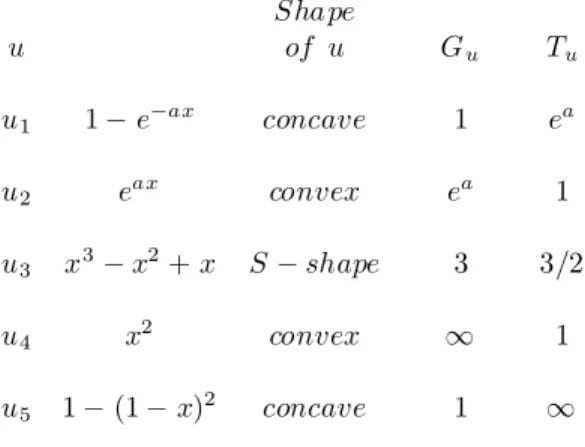
For reasons of simplicity, we assume that C = [0; 1]. We propose …rst some functions u in Table 2 and ' in Table 3 and their respective indexes.
Table 2 : Some examples of u functions and their indexes
Shape u of u Gu Tu u1 1¡ e¡ax concave 1 ea u2 eax convex ea 1 u3 x3¡ x2+ x S¡ shape 3 3=2 u4 x2 convex 1 1 u5 1¡ (1 ¡ x)2 concave 1 1
Table 3 : Some examples of ' functions and their indexes ' shape of ' P ' O' '1 p3 ' 1(p)· p 3 irrel: and convex '2 p+( 1p¡p)µ '2(p)· p µ irrel: µ¸ 1 and convex '3 1¡ (1 ¡ p)3 '3(p)¸ p irrel: 3 and concave
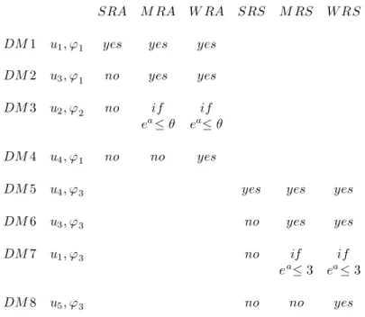
Examples of some diversi…ed attitudes towards risk in RDU In the following table, we show how di¤erent combinations of the previous utilities and probability weighting functions illustrate di¤erent types of risk aversion/risk seeking in the RDU model.
Table 4 : Examples of DM’ attitudes SRA M RA W RA SRS M RS W RS DM 1 u1; '1 yes yes yes
DM 2 u3; '1 no yes yes
DM 3 u2; '2 no if if
ea· µ ea· µ
DM 4 u4; '1 no no yes
DM 5 u4; '3 yes yes yes
DM 6 u3; '3 no yes yes
DM 7 u1; '3 no if if
ea· 3 ea· 3
DM 8 u5; '3 no no yes
These examples show that:
(i)A RDU DM, with a unique marginal utility with diminishing parts and increasing parts (like u3, in the examples), can have Monotone Risk Aversion
(thus Weak Risk Aversion), if su¢ciently pessimistic (like for DM2 with (u3,'1))
and Monotone Risk-Seeking (thus Weak Risk-Seeking), if su¢ciently optimistic (like for DM6 with (u3, '3)).
(ii) Weak risk Aversion does not imply necessarily Monotone Risk Aver-sion like for DM4 and similarly, Weak Risk-Seeking does not imply necessarily Monotone Risk-Seeking like for DM8. The properties of the two last exam-ples are proved in Chateauneuf, Cohen and Meilijson (2006). However, in the same paper, they show that, in fact, there is few room for Weak Risk Averse DMs that are not Monotone Risk Averse, so that Monotone Risk Aversion can capture most of the Weak Risk Averse attitudes.
5.5 Adequation of observed behavior to the RDU model
This RDU model under risk, will not only prove to be compatible with ob-served behaviors in Allais’ paradox, but also, in some cases, compatible with many observed attitudes, already mentioned in the section 4.3.2. that are not explainable in the EU model.
5.5.1 Explanation of Allais’ paradox
It can be easily proved that Allais’ paradox is explainable by RDU theory. In the example given in section 4, any DM choosing simultaneously A and D conform with the RDU model, as soon as his ' satis…es:
'(0; 8) = '(0;200;25) < '(0;20)'(0;25)
Indeed, with the normalization u(4000) = 1;u(0) = 0 and denoting ® = u(3000); we have V (A) = ®; V (B) = '(0; 8); V (C ) = ®'(0; 25); V (D) = '(0; 20) and thus, A Â B and D Â C , as soon as ® > '(0; 8) and ®'(0; 25) < '(0; 20); which gives the result above.
5.5.2 Adequation of other observed behaviors
RDU model can thus answer to several criticisms raised by the EU model : (1) In the examples, we have seen that the RDU model can explain the behavior of a Monotone Risk-Seeking (or Weak Risk-Seeking) DM with a di-minishing marginal utility: see, for instance the behavior of DM7 where u is concave (with ea· 3)and ' reveals optimism.
(2) We have seen, in the examples, that a DM can have Weak Risk Aversion without having Strong Risk Aversion: see, for instance the behavior of DM2 or DM4.
(3) RDU model is constructed to take into account the link between per-ceived probabilities and consequences. The intensity of variation between given probabilities and perceived probabilities are well taken into account by the prob-ability weighting function '. Moreover, to take into account that, for the same probability, perception of risk can depend on the decision problem the DM is facing, the function ' can depend on a parameter s, indicating the in‡uence of the context, past experience, framing, feelings of the DM.... For example, if s indicates the level of the danger, 's can be more (less) optimist if the danger
is more (less) controlled ; if s indicates the level of knowledge or familiarity of the danger, again, 's can be more (less) optimist if the danger is more (less)
familiar. A formalization of attitudes characterized by (u;'s), where s indicates
the past-experience, can be found in Cohen, Etner, Jeleva (2006).
(4) Finally, let us just mention, among others, an observed economic behavior explained in the framework of RDU: it can be optimal for a policy holder to buy a complete insurance coverage, even when the premium is loaded, if he is su¢ciently pessimistic under risk.
5.6 Assessment of the di¤erent parameters
In a perspective of Decision Aiding, the next step to help each Decision Maker to take an optimal decision is to assess his di¤erent parameters in the RDU model.
' is the identity. We thus can use the same experimental method for all DMs. Unfortunately, the assessment of the two parameters u and ' are linked and we need a sequential experiment to assess simultaneously the two functions. There exists sophisticated methods to achieve this goal (Wakker and Dene¤e, 1996).
From an empirical point of view, the perception function ' has been assessed, …rst at a global level, by, among others, Abdellaoui (2000), Tversky and Wakker (1995), Wu and Gonzalez (1996), and axiomatically justi…ed by Prelec (1998).
Then, experimental studies have been conducted, at an individual level, to assess the two functions of the DM in di¤erent types of consequences and con-text: monetary gains in Abdellaoui (2000), risks of monetary losses with dif-ferent levels of losses in Etchard-Vincent (2004), risk of bad consequences of medical decisions in Bleichrodt and Pinto (2000), probabilities based on QALY (Quality Adjusted Life Year) in Bleichrodt and Quiggin ((1997), risk of nu-clear accidents in nunu-clear power plant maintenance in Beaudouin, Munier and Serquin (1999). They show not only heterogeneity in individual preferences,but also heterogeneity according to the di¤erent contexts of the experiment.
The last study (De Lapparent, 2006) concerns the risk of time loss in travel activity (for air route choices) and it is an empirical one, based on a large data base. De Lapparent (2006) prove that (i) travellers choices are not compatible with EU theory but compatible with RDU theory (ii) that travellers are opti-mistic under risk ('(p) ¸ p) which is interesting because this optimism can be interpreted as a signal of trust that passengers have, concerning their airline company.
6 Concluding remarks
We have seen that RDU model accounts for many observed behaviors under risk. However, this model has a drawback: it is not dynamically consistent.
A solution to deal with a dynamic model with RDU static preferences is to use a recursive model a la Kreps-Porteus. Moreover, in such a recursive model, we can take into account the possible evolution, during time, of the risk perception, more particularly the in‡uence that history of each DM can have on this perception. Cohen, Etner, and Jeleva [2006] have studied such a model and their illustration by an insurance problem shows that this dynamic model can explain changes in behavior about insurance coverage, observed in real behaviors, that are not explainable in the other classical models.
References
[1] Abdellaoui, M.(2000). Parameter-free elicitation of utilities and probabili-ties weighting functions, Management Science, 46, 11, 1497-1512.
[2] Allais, M.(1953). Le comportement de l’homme rationnel devant le risque: critique des postulats et axiomes de l’école américaine, Econometrica, 21, 503–546.
[3] Allais, M.(1988)The general theory of random choices in relation to the invariant cardinal utility function and the speci…c probability function, in Risk, Decision and Rationality, B. R. Munier (Ed.), Reidel: Dordrech, 233– 289.
[4] Beaudouin, F., B. Munier et Y. Serquin, (1999). Multi-Attribute Decision Making and Generalized Expected Utility in Nuclear Power Plant Mainte-nance , in: M. Machina, B. Munier, eds., Beliefs, Interactions and Prefer-ences in Decision Making, Dordrecht/Boston, KAP.
[5] Bleichrodt, H. and J. Quiggin (1997). Characterizing QALYs under a Gen-eral Rank Dependent Utility ModelJournal of Risk and Uncertainty Vol-ume 15, 2.
[6] Bleichrodt, H. and JL. Pinto (2000). Parameter-Free Elicitation of Utility and Probability Weighting FunctionsManagement Science, Volume 46, 11. [7] Chateauneuf, A. (1999). On the use of comonotony in the axiomatization of EURDP theory for arbitrary consequencesJournal of Mathematical Eco-nomics, 32.
[8] Chateauneuf, A. and M. Cohen (1994). Risk seeking with diminishing mar-ginal utility in a non-expected utility model, Journal of Risk and Uncer-tainty,9, 77–91.
[9] Chateauneuf, A., M. Cohen and I. Meilijson, (2004). Four notions of mean preserving increase in risk, risk attitudes and applications to the Rank-Dependent Expected Utility model , Journal of Mathematical Economics, 40, p 547-571.
[10] Chateauneuf, A., M. Cohen and I. Meilijson, (2005).More pessimism than greediness: A characterization of monotone risk aversion in the Rank De-pendent Expected Utility model , Economic Theory, 25, 649-667.
[11] Chateauneuf, A., M. Cohen and I. Meilijson, (2006).Weak risk aversion and the quest for simplicity: A characterisation of the preference for safety in the RDU model: WorkingPaper:
[12] Chew, S., E. Karni and Z., Safra (1987). Risk aversion in the theory of expected utility with Rank Dependent preferences, Journal of Economic Theory,42, 370–381.
[13] Choquet, G, (1953). Theorie des capacités, Ann. Institut Fourier (Greno-ble),V, 131-295.
[14] Cohen, M. , J. Etner and M. Jeleva , (2007). Dynamic Decision Making when Risk Perception Depends on Past Experience, to appear in Theory and Decision.
[15] de Lapparent, M. (2006) Optimism, pessimism towards risk of time losses in business air travel demand, to appear in Intelligent Transportation Systems : [16] Ellsberg, D., (1961). ” Risk, Ambiguity, and the Savage Axioms”, The
Quarterly Journal of Economics, p643-669.
[17] Etchart-Vincent, N. (2004).Is Probability Weighting Sensitive to the Mag-nitude of Consequences ? An Experimental Investigation on Losses,Journal of Risk and Uncertainty, vol. 28(3).
[18] Jewitt, I., (1989). Choosing between risky prospects: the characterisation of comparative static results and location independent risk. Management Science, 35, 60–70.
[19] Kahneman, D., & Tversky, A. (1979). Prospect theory: An analysis of decisions under risk. Econometrica, 47, 263-291.
[20] Knight, F (1921). Risk, Uncertainty and Pro…t., University of Chicago Press.
[21] Kreps, D. (1988). Notes on the theory of choice. Boulder and London, West-view Press.
[22] Landsberger, M. and I. Meilijson.(1994). Comonotone allocations, Bickel-Lehmann dispersion and the Arrow-Pratt measure of risk aversion, Annals of Operations Research,52, 97–106.
[23] Landsberger, M. and I. Meilijson, (1994). The generating pro cess and an extension of Jewitt’s location independent risk concept. Management Sci-ence,40, 662–669.
[24] C Menezes, C Geiss and J. Tressler (1980). Increasing Downside Risk, American Economic Review, vol. 70, n±5, p 921-932.
[25] Prelec, D. (1998) The probability weighting function, Econometrica, 66, 3, p497-527.
[26] Quiggin, J.(1982) A theory of anticipated utility,Journal of Economic Be-havior and Organisation,3, 323–343.
[27] Quiggin, J.(1992) Increasing risk: another de…nition, In Progress in Deci-sion, Utility and Risk Theory, A. Chikan (Ed.), Dordrecht: Kluwer. [28] Rothschild, M. and J. Stiglitz (1970). Increasing Risk: I. A de…nition,
Jour-nal of Economic Theory, 2, 225–243.
[29] Rothschild, M. and J. Stiglitz (1971).Increasing Risk II: Its economic con-sequences, with J.E. Stiglitz Journal of Economic Theory, 3,1.
[31] Tversky, A. and P. Wakker.(1995) Risk attitudes and decision weights, Econometrica, 63, 6, p1255-1280.
[32] von Neumann J. and O. Morgenstern (1944). Theory of Games and Eco-nomic Behavior. New York: John Wiley and Sons.
[33] Wakker, P.(1994) Separating marginal utility and risk aversion, Theory and Decision,36, 1–44.
[34] Wakker, P. P., D. Dene¤e. (1996). Eliciting von Neumann-Morgenstern utilities when probabilities are distorted or unknown. Management Science, 42, 1131–1150.
[35] Weber, E. U. (1997). The utility of measuring and modeling perceived risk. In A. A. J. Marley (Ed.), Choice, Decision, and Measurement: Essays in Honor of R. Duncan Luce (p45-57). Mahwah, NJ: Lawrence Erlbaum Associates.
[36] Weber, E. U., Blais, A.-R., & Betz, N. (2002). A domain-speci…c risk-attitude scale: Measuring risk perceptions and risk behaviors. Journal of Behavioral Decision Making, 15, 1-28.
[37] Wu, G. and R. Gonzalez. (, 1996). Curvature of the probability weighting function, Management Science, 42, 1676-1690.
[38] Yaari, M.(1987). The dual theory of choice under risk, Econometrica, 55, 95–115.