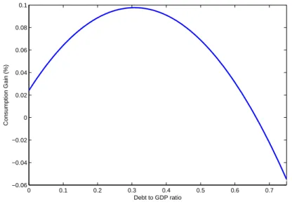
Public debt and aggregate risk

Denition 1: Given scientic knowledge F , a utility function on the space of consequences, and a set of acts , measurable with respect to F and nor- malized in such a way that and act

Fully developed green leaves of the 8 most abundant grass species (Lolium perenne, Phleum pratense, Festuca pratensis, Lolium multiflorum, Poa pratensis, Dactylis glom- erata,

In general, subjects with a poor health at baseline showed a larger increase in health after re-employment than subjects with a good health at baseline (data not shown).However,

In the mean field description of the incommensurate transition of quartz, the triangular 3-q, the striped I-q and the fl phases meet at the same critical point.. It is shown

L’étude concerne des patients diabétiques qui consultaient au service d’endocrinologie de l’Hôpital Militaire d’Instruction Mohammed V, ainsi que ceux

Results show that the correlation between charge and temperature fluctuations significantly affect the thermal balance for nm-sized particles.. We also showed that

In particu- lar, when absolute risk aversion is decreasing, lowering the resistance to intertem- poral substitution from the intertemporal utility maximizing level, so that ρ(x)

In par- ticular, when absolute risk aversion is decreasing, lowering the resistance to intertemporal substitution from the intertemporal utility maximizing level, so that ρ( x)