Is Our World Going to Get a Whole Lot Smaller?
43
0
0
Texte intégral
(2) CIRANO Le CIRANO est un organisme sans but lucratif constitué en vertu de la Loi des compagnies du Québec. Le financement de son infrastructure et de ses activités de recherche provient des cotisations de ses organisations-membres, d’une subvention d’infrastructure du Ministère du Développement économique et régional et de la Recherche, de même que des subventions et mandats obtenus par ses équipes de recherche. CIRANO is a private non-profit organization incorporated under the Québec Companies Act. Its infrastructure and research activities are funded through fees paid by member organizations, an infrastructure grant from the Ministère du Développement économique et régional et de la Recherche, and grants and research mandates obtained by its research teams. Les partenaires du CIRANO Partenaire majeur Ministère du Développement économique, de l’Innovation et de l’Exportation Partenaires corporatifs Banque de développement du Canada Banque du Canada Banque Laurentienne du Canada Banque Nationale du Canada Banque Royale du Canada Banque Scotia Bell Canada BMO Groupe financier Caisse de dépôt et placement du Québec Fédération des caisses Desjardins du Québec Financière Sun Life, Québec Gaz Métro Hydro-Québec Industrie Canada Investissements PSP Ministère des Finances du Québec Power Corporation du Canada Raymond Chabot Grant Thornton Rio Tinto State Street Global Advisors Transat A.T. Ville de Montréal Partenaires universitaires École Polytechnique de Montréal HEC Montréal McGill University Université Concordia Université de Montréal Université de Sherbrooke Université du Québec Université du Québec à Montréal Université Laval Le CIRANO collabore avec de nombreux centres et chaires de recherche universitaires dont on peut consulter la liste sur son site web. Les cahiers de la série scientifique (CS) visent à rendre accessibles des résultats de recherche effectuée au CIRANO afin de susciter échanges et commentaires. Ces cahiers sont écrits dans le style des publications scientifiques. Les idées et les opinions émises sont sous l’unique responsabilité des auteurs et ne représentent pas nécessairement les positions du CIRANO ou de ses partenaires. This paper presents research carried out at CIRANO and aims at encouraging discussion and comment. The observations and viewpoints expressed are the sole responsibility of the authors. They do not necessarily represent positions of CIRANO or its partners.. ISSN 1198-8177. Partenaire financier.
(3) Is Our World Going to Get a Whole Lot Smaller? Byron S. Gangnes *, Alyson C. Ma †, Ari Van Assche ‡. Abstract. The surge of oil prices in recent years has led to speculation that rising transportation costs could end the period of dramatic world trade growth — in the words of Rubin (2009), “…Your world is going to get a whole lot smaller.” Using data from China’s Customs Statistics, we examine the impact of oil prices on trade’s sensitivity to distance. We find that higher oil prices increase trade’s elasticity to distance, but that the economic effect is small. We also find that the effect is more pronounced for trade within global production networks, and less large for goods shipped by air.. Keywords: oil prices, distance, trade, vertical specialization, mode of transport, China. *. University of Hawaii at Manoa; Visiting Professor, Yokohama National University University of San Diego ‡ Corresponding author. HEC Montréal, Katholieke Universiteit Leuven and CIRANO. Address: HEC Montréal, Department of International Business, 3000 Chemin de la Côte-Sainte-Catherine, Montréal (Québec), Canada H3T-2A7. Phone: (514)340-6043. Fax: (514)340-6987. E-mail: [email protected] †.
(4) 1. Introduction In the six years leading up to the global recession of 2009-2010, oil prices rose dramatically, from an annual average of roughly US$26 a barrel in 2002 to nearly US$100 a barrel in 2008. In the summer of 2008, prices briefly spiked to nearly US$150 per barrel before receding as the recession deepened. As oil prices surged upward in 2008, business analysts became increasingly worried about the impact of rising oil prices on trade. Rubin and Tal (2008) of CIBC World Markets wrote a thought-provoking article that rising oil prices will lead to significant hikes in international transportation costs and therefore to a major slowdown in the growth of world trade—reversing globalization.1 They reported that hand-in-hand with the oil price hikes, the cost to ship a standard 40-foot container from Shanghai to the U.S. eastern seaboard rose from US$3,000 in 2000 to US$8,000 in 2008. At such transport prices, they argued, companies have started to rethink the establishment of far-flung global supply networks, by seeking supplies from domestic and regional markets closer to home. Following on the heels of Rubin and Tal (2008), Jen and Bindelli (2008) of Morgan Stanley Research predicted that East Asia‘s and especially China‘s export model would be particularly affected by rising oil prices. This is because trade within East Asia is much more vertically specialized than for other regions. Many of the finished goods that China exports to America and Europe are made from components imported from Taiwan, Japan and South Korea. Since these regional production networks require components to. 1.
(5) be shipped multiple times, affordable transport costs are an essential ingredient for their maintenance. Other experts and practitioners, however, have argued that the impact of rising oil prices on trade will be relatively limited, and will depend on the type of product (Economist, 2008; Murphy, 2008). There are more reasons for a company to go global than just cut labor cost. The impact of oil prices on offshoring decisions depend on the weight and the value of the goods being transported, as well as the extent of other advantages like quality, responsiveness, and access to local markets (Murphy, 2008). Perhaps surprisingly, academic research on the role of oil price changes on trade has remained scant. In this paper, we take advantage of a unique panel data set from China Customs Statistics for the period from 1988 to 2008 to investigate the impact of oil prices on Chinese trade. The data set is of interest for a number of reasons. First, because this dataset distinguishes between ―normal‖ trade and processing trade, we are able to test Jen and Bindelli‘s (2008) conjecture that trade within global production networks is more sensitive to oil prices than other trade flows. Second, data on transport mode permit us to evaluate potential differences in oil price effects for goods with high value-weight ratios and goods that are time sensitive. Finally, since China is among the world‘s largest trading nations, our study will allow us to gain new insights into whether rising oil prices threaten to have a significant impact on world trade‘s sensitivity to distance. We find evidence that China‘s exports indeed have become more sensitive to export distance in times of rising oil prices. We also find that these effects are more pronounced for processing exports, where goods must cross borders multiple times. On the other hand, we find that goods shipped by air are less vulnerable to these effects, consistent 2.
(6) with their higher value-to-weight ratio and the relatively greater importance of factors other than transportation cost—such as timeliness—for these goods. While these results are statistically significant, their economic effects are relatively small. We estimate that the quadrupling of oil prices between 2002 and 2008 has increased the elasticity of Chinese exports to distance by a mere 5-7%. Our analysis therefore suggests that the concerns of business analysts that rising oil prices will significantly increase trade‘s sensitivity to distance are likely overblown. The paper is organized as follows. In the next section, we review the literature and develop our research hypotheses. In section 3, we discuss the data. In section 4, we present our methods. In section 5, we present the results. Section 6 concludes.. 2. Research hypotheses 2.1. Oil prices, transport costs and trade There has been an enormous expansion in world trade during the past half century. The value of world merchandise exports first exceeded $US 1 trillion in 1977, and by 2008 more than 16 trillion current US dollars of merchandises were exported. During the same time period, the share of the world GDP accounted by merchandise trade surged from 18% to 52%. In addition to standard explanations that focus on reductions in tariff and non-tariff barriers or rising world income, one candidate explanation for the rapid growth of world trade is a trend decline in transportation costs. Hummels (2007) shows that a substantial decline in shipping costs occurred in the post-war period, largely due to technological changes. The decline was most dramatic for air shipping costs, where the cost per ton fell. 3.
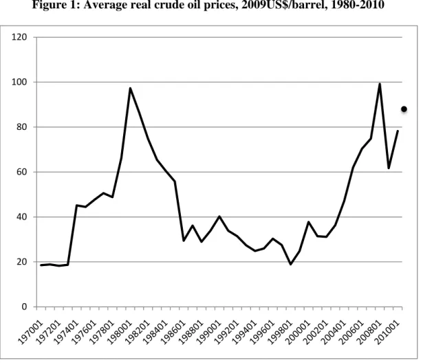
(7) from $3.87 per ton-kilometer in 1955 to under $0.30 by 2004, according to data from the International Air Transportation Association. As Gordon (1990) had observed earlier, the drop was particularly sharp in the 1955-72 period, when the jet engine replaced much more expensive piston engine aircraft, but costs continued to decline at a 3.5% annual rate during the 1972-2003 period (the rate of decline is somewhat smaller when US Bureau of Labor Statistics price index data is used). A decline in waterborne shipping prices is less obvious in the raw data, although there is evidence that containerization reduced shipping costs significantly below what they would otherwise have been during the 1974-2004 period. Some now argue that this trend of trade expansion will be reversed in the near future. Rubin and Tal (2008) and Rubin (2009) have argued that rising oil prices are likely to lead to significant hikes in international transportation costs and therefore to a major slowdown in the growth of world trade. Clearly how large these effects are going forward will depend on the extent of future oil price increases, the impact of rising oil prices on transport costs, and the sensitivity of trade to these changing costs. Oil prices have risen dramatically in the last decade. As shown in Figure 1, while crude oil prices in real terms were relatively low from the mid-1980s through the 1990s, they increased rapidly thereafter, more than tripling between 2002 and 2008. Oil prices retreated sharply during the Global Recession of 2008-2009, but as many expected (Adams, 2009), they have since recovered to relatively high levels as global economic growth has resumed. [Figure 1 about here]. 4.
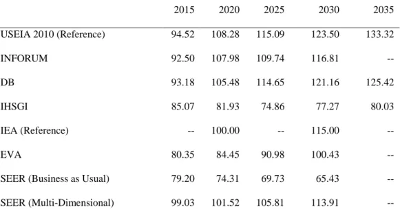
(8) While there is considerable uncertainty about the future path of oil prices, there is a fairly broad consensus that prices will rise further in coming years, as limited oil supply meets continuing robust growth in energy demand from the developing world. In fact, a large number of oil experts predict that the world will see ―peak oil‖, the maximum level of conventional oil output (i.e. excluding heavy oil from tar sands, oil shale etc.), within the next decade (De Almeida and Silva, 2009). Supply responses by oil producers and the adoption of alternative energy technology may fill part of the ensuing gap, but in any case there will likely be persistent upward pressure on oil prices. Table 1 reports oil price forecasts from a number of leading government agencies and firms (US Energy Information Agency, 2010). In the majority of projections, oil prices measured in 2008 dollars are expected to exceed $90 per barrel by 2015 and $100 per barrel by 2020, with further increases thereafter. None of the forecasts see oil prices returning to the low levels experienced during the 1985-2000 period.. [Table 1 about here]. How much will higher oil prices change effective transportation costs? Here the evidence is mixed, but some studies have estimated a sensitivity of shipping freight rates to oil prices that is relatively low, potentially limiting the threat that rising oil prices will lead to a significant reduction in the growth of trade. Hummels (2007) and UNCTAD (2010) estimate an elasticity of maritime cargo costs with respect to fuel prices between 0.20 and 0.40. Mirza and Zitouna (2009) estimate an even lower elasticity of freight rates to oil prices ranging from 0.02 to 0.15. Taking Hummels (2007) estimate of 0.20, the near quadrupling of oil prices that occurred between 2002 and 2008 (prices rose 282% on an. 5.
(9) annual basis) would have raised shipping costs by 56%. While perhaps far from crippling, clearly there is likelihood of significantly higher transport costs in coming years. Given higher transportation costs, the question is to what extent this will reduce trade. We will have more to say about this below, when we discuss the differential effects on transportation cost on alternative shipping modes. Rubin and Tal (2008) observe that trade growth dropped to zero during the period of high oil prices in 1974-1986, compared with the rapid trade expansion of the 1960-1973 and 1987-2002 periods. While the deep global recessions of 1974 and 1981-82 certainly held back trade, they argue that the failure of trade to rebound following the recessions was largely due to surging transport costs associated with sharply higher oil prices. Looking at more recent experience, they estimate that China‘s exports to the U.S. during the 2004-2007 would have been 30% higher in the absence of the sharply rising oil prices.2 Everything else being equal, the effect of rising oil prices should fall more heavily on freight-intensive distant trade rather than proximate trade. Rubin and Tal (2008) show that there was a geographical shift of U.S. trade away from Asia and Europe to Latin America and the Caribbean during the 1974-1986 period. This leads us to our first testable hypothesis:. Hypothesis 1: Ceteris paribus, a rise in oil prices increases the sensitivity of trade to distance.. This can be assessed using a variant of the standard gravity model of trade, as we will discuss below. 6.
(10) 2.2. Oil prices and the nature of trade The nature of world trade has changed significantly in recent years. While for centuries manufactured goods trade primarily entailed an exchange of finished products that were each produced within a single country, today it increasingly involves the exchange of parts and components at various stages of an internationally dispersed production process.3 Thanks to reductions in tariffs, communication and transport costs, and other trade barriers, multinational firms now often slice up their supply chains, with bits of value added generated in many different locations around the globe. This has led to a rapid growth in vertically specialized trade between different nodes of the same global production network (GPN) (Feenstra, 1998; Hummels et al., 2001). The rise of GPNs is most evident in electronics (Sturgeon, 2002; Gangnes and Van Assche, 2010). An Apple video iPod, for example, may have its final assembly in China, but includes components made in the United States, Japan, Korea, Taiwan and Singapore (Linden et al., 2009). But the emergence of GPNs extends well beyond electronics to automobiles, toys and many other products. Hummels et al. (2001) found that the import content of exports accounted for nearly 21% of the exports of ten OECD and four emerging countries in 1990 and grew almost 30% between 1970 and 1990. Using more recent data, Miroudot and Ragoussis (2009) found that the average import content of exports has risen from 26% in 1995 to 31% in 2005. A rise in oil prices may affect trade within GPNs differently from non-GPN trade. Hummels et al. (2001) and Yi (2003) have argued that intra-GPN trade should be more sensitive than regular trade to changes in tariffs, transportation costs and other trade barriers, since the fragmentation of the production process leads to goods crossing 7.
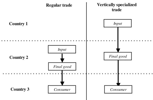
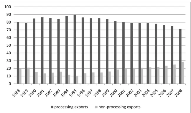
(11) borders multiple times. To illustrate this, consider Figure 2. The left panel shows a traditional trade pattern where a product is entirely produced in country 2 and then exported to country 3 for consumption. The right panel shows a vertically specialized trade pattern within a GPN. Country 1 produces inputs and exports them to country 2. Country 2 uses the imported inputs to produce a final good. Finally, country 2 exports its output to country 3 for consumption. In the latter case, the input produced in country 1 ends up crossing borders two times, leading to a multiplication of trading costs. Hummels et al. (2001) and Yi (2003) introduced this argument as a potential explanation for how tariff (and possibly transportation cost) reductions may explain a larger proportion of measured trade growth than predicted by traditional trade models. But the converse is also true: an increase in transportation costs could lead to a magnified increase in production costs and therefore decrease disproportionately intra-GPN trade.. [Figure 2 about here]. Using this reasoning, Jen and Bindelli (2008) of Morgan Stanley Research predicted that East Asia‘s and especially China‘s export model would be particularly affected by rising oil prices, since East Asian trade is much more vertically specialized than for other regions (Athukorala and Yamashita, 2006; Haddad, 2007). As supporting evidence, they reported that the share of China‘s exports that are processing exports fell from about 57% in late 2001 to 44% in mid-2008, moving in roughly inverse relationship with oil prices. This leads to our second hypothesis:. Hypothesis 2: Ceteris paribus, a rise in oil prices increases the sensitivity of trade to distance more for intra-GPN trade than for regular trade. 8.
(12) As we describe further below, we can compare data on Chinese exports from processing zones to non-processing exports to evaluate this hypothesis.. 2.3. Oil prices and transport mode Oil price changes may also differentially impact trade depending on the types of goods that are traded. Two types of goods in particular may be less sensitive to oil price changes: goods with a high value-to-weight ratio and goods with a high utility value of timely delivery. These goods are more likely to be shipped by air than is the typical good. The prevalence of air transport has increased markedly in recent decades. As a share of value, the proportion of US exports shipped by air rose from about 12% in 1965 to nearly 53% in 2004 (Hummels, 2007). One reason for this rapid expansion has been a steep drop in the relative price of air to ocean shipping, down 40% between 1990 and 2004 (Harrigan, 2010).. Across the range of manufactured goods, weight-to-value has also. fallen (Hummels, 2007), presumably reflecting the evolving composition of global consumption toward, for example, high value electronics goods. The time sensitivity of trade also appears to have increased, perhaps because of the shift toward complex manufactures and the need to respond quickly to the increasingly precise and volatile product demands of a more affluent global society (Hummels, 2007). Falling costs per unit value and rising utility value of timeliness mean that still-costly air transport can be justified for a larger number of goods than in the past. The characteristics of goods shipped by air likely make them less sensitive to changes in transportation costs than goods shipped by water. Shipping costs depend primarily on the. 9.
(13) physical characteristics of a product rather than on its value. As a result, goods with a higher value-to-weight ratio have a lower shipping cost per unit of value (Hummels, 2007; Harrigan, 2010). For these goods, an increase in the shipping costs therefore has a less severe impact on total costs, making their price less sensitive to transport cost changes. Similarly, goods with a high utility value of time may be less sensitive to shipping cost changes since the importance of timeliness trumps at least in part cost considerations (Hummels and Schaur, 2010). This allows us to frame our third hypothesis.4 Hypothesis 3: Ceteris paribus, a rise in oil prices increases the sensitivity of trade to distance less for products shipped by air than for products shipped by sea.. 3. Data Description To test our hypotheses, we use a unique trade dataset from China‘s Customs Statistics.5 This dataset captures all China‘s international trade transactions between 1988 and 2008 inclusive. It records for each flow of goods across China‘s border the product classification, the value and quantity shipped, the year of shipment, the Chinese province of origin and the destination country (Feenstra et al., 2004). In addition, it provides information on the customs regime under which an international flow takes place and its mode of transportation. To test our hypotheses, we take advantage of the panel structure of the international trade data to investigate whether rising oil prices in the early twenty-first century have rendered China‘s exports more sensitive to distance-related trade costs. Furthermore, as we will discuss in this section, we will use information on the customs regime and on the. 10.
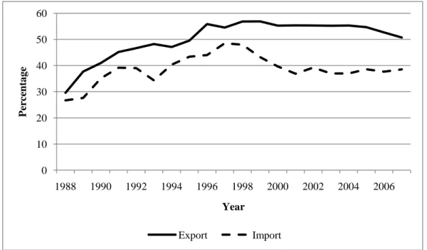
(14) mode of transportation to investigate if the nature of trade and the type of goods play a mediating role on the impact of oil prices on trade.. 3.1. Processing trade vs. non-processing trade A unique characteristic of our Chinese trade dataset is that it differentiates between trade that occurs under China‘s processing trade regime and other (non-processing) trade. This differentiation is important since processing trade transactions unambiguously reflect intra-GPN trade.6 In the mid-eighties, the Chinese government instituted the processing trade regime to entice foreign firms to offshore their production activities to China, while protecting the domestic market from foreign competition. Under this regime, firms located in China are granted duty exemptions on imported raw materials and other inputs as long as they are used solely for export purposes. Since firms can only use this customs regime if they import components for export purposes, processing exports clearly reflect intra-GPN trade. Four stylized facts highlight the relative size and distinctive nature of China‘s processing trade versus non-processing trade. First, as it is shown in figure 3, the share of processing exports (i.e. exports conducted under the processing regime) in China's total exports has risen from 30% in 1988 to 51% in 2008, while the share of processing imports in total imports has increased from 27% to 38%. In other words, more than half of China‘s exports are currently intra-GPN trade.. [Figure 3 about here]. Second, processing exports rely more heavily on imported inputs than non-processing exports. In a recent paper, Koopman et al. (2008) combined the China Customs Statistics 11.
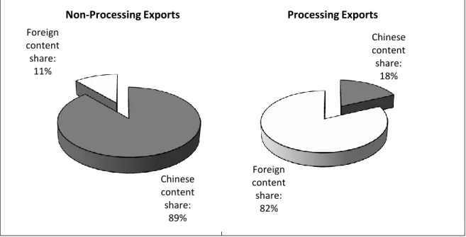
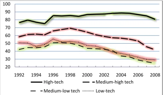
(15) trade data with an input-output table for China to estimate the domestic content share of China‘s processing and non-processing exports. As it is shown in Figure 4, they found that, in 2006, the domestic content share of processing exports was merely 18.1%, implying that the value of imported inputs accounted for 81.9% of the processing export value. Conversely, the domestic content share of non-processing exports stood at a much higher 88.7%, meaning that imported inputs only represented 11.3% of the export value.. [Figure 4 about here]. Third, processing exports are predominantly conducted by foreign invested enterprises (FIEs),7 whereas non-processing exports are largely conducted by local firms. Between 1992 and 2008, the share of processing exports conducted by FIEs has varied from a high of 89.7% in 1995 to a low of 71.4% in 2008 (see Figure 5). Conversely, FIEs‘ share of non-processing exports has consistently remained below 30%.. [Figure 5 about here]. Fourth, processing exports are more intensively used in high-technology industries such as electronics. To demonstrate this, we have used the Organization of Economic Cooperation and Development‘s (OECD) technology classification (Hatzichronoglou, 1997) to disaggregate China‘s exports into four categories: high technology exports, medium-high technology exports, medium-low technology exports and low technology exports.8 In Figure 6, we depict the share of processing exports in China‘s total exports for each technology category. Tellingly, processing exports are more important in higher technology categories than in lower technology categories. In 2008, processing exports. 12.
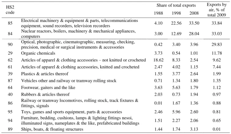
(16) accounted for 80.6% of high-technology exports; 41.9% of medium-high-technology exports; 28.9% of medium-low-technology exports; and 24.7% of low-technology exports. The high prevalence of processing exports in high-technology industries is largely due to electronics companies‘ decisions to offshore their labor-intensive assembly operations in China (Gangnes and Van Assche, 2010). In 2008, two thirds of China‘s high-technology goods exported under the processing trade regime was electronics goods.9 [Figure 6 about here]. These distinctions between processing trade and non-processing trade suggest that China‘s foreign trade regime has effectively turned into a dualistic system (Ma and Van Assche, 2011). In higher technology industries, foreign firms have on a large scale used China‘s processing trade regime to integrate the country into their GPNs. In these industries, China heavily relies on imported inputs and is primarily responsible for the labor-intensive downstream activities such as assembly. Conversely, in lower technology industries, China is relatively uninvolved in GPNs, with its exports largely conducted outside the processing trade regime by domestic firms that source their inputs locally. In our empirical analysis below, we will assess whether these two types of trade are affected differently by oil price increases.. 3.2. Mode of transportation Information on the mode of transportation allows us to investigate whether air trade is less sensitive to oil price changes than ocean trade. To differentiate between air and ocean trade, we disaggregate our trade data into industries that intensively use air. 13.
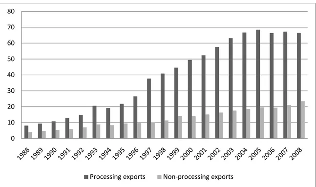
(17) transport and industries that do not. For this purpose, we use the 2009 trade data from China‘s Customs Statistics to calculate for each industry at the 2-digit HS level the share of China‘s exports to nonadjacent countries that is shipped by air.10 The results are presented in table 2 (the table only retains the HS 2-digit industries that represent more than 1% of the export share in 2008). The table shows that air transport is significantly more important for industries that produce goods with a high value-to-weight ratio and just-in-time production. Specifically, for electronics industries such as computers (84), telecommunications equipment (85) and electronic instruments (90), air transport is an important transport mode. Conversely, products with a low value-to-weight ratio (apparel, footwear, toys, furniture) and bulk commodities like iron and steel and (of course) ships are exported entirely or nearly entirely by sea.. [Table 2 about here]. Notice that the air-intensive industries are also the industries that are more heavily integrated into global production networks. In Figure 7, we show the share of exports that are in air-intensive industries by processing exports and non-processing exports respectively. In 2008, more than 65 percent of processing exports were in air-intensive industries, while this number was less than 25 percent for non-processing exports.. [Figure 7 about here]. 4. Empirical Specification Hypothesis 1 states that all else equal, a rise in oil prices increases the sensitivity of trade to distance. To test this, we estimate the following equation for the years 1988-2008:. 14.
(18) . where the dependent variable province i to country j in year t,. is the natural log of the value of exports from is a constant term,. are destination country fixed effects, country j‘s GDP in year t,. (1). are province-time fixed effects,. is the natural log of the destination. is the average crude oil price in US$/barrel in year t and. measures the distance between China and destination country j. Table 3 presents descriptive statistics and data sources.. [Table 3 about here] Equation (1) is a variant of the workhorse gravity model of trade.11 Our estimation approach takes into account two recent methodological innovations in the gravity model literature. Egger (2002), Anderson and van Wincoop (2003, 2004) and Anderson (2011) have shown that omitting controls for multilateral resistance can create severe biases on distance estimates in a gravity setting.12 They have called for the inclusion of timevarying origin and destination fixed effects to control for this. In our estimation equation, we therefore include province-time fixed effects and country fixed effects.13 These fixed effects imply that our estimation equation excludes a number of variables that are traditionally used in gravity models. For example, the province-time fixed effects capture the impact of any time-varying variable specific to a Chinese province, including its respective GDP per capita, population size, real wages, landlocked status and institutional features. Similarly, the country fixed effects capture the effect of time non-varying country-specific variables such as its size, the degree of home bias and the multilateral resistance term.14 A disadvantage of including these fixed effects is that they prevent 15.
(19) separate estimation of the coefficients on export distance ( (. ) and oil prices. ). Since export distance to a given country is similar for all Chinese provinces,. distance is country-specific in our dataset, and is therefore captured by the country fixed effects. Similarly, since oil price changes are identical for all Chinese provinces, their effect is captured by the province-time fixed effects. This is not of a great concern since our estimation equation still allows us to investigate the relative impact of oil price changes on China‘s trade mediated through distance (with the interaction term ). In other words, we can still investigate whether, during times of oil prices increase, Chinese exports become more sensitive to distance. Hypothesis 1 will be supported if. is negative and significant.15. Our estimation approach also deals with a second estimation problem that has recently gained attention in the gravity literature. The standard OLS procedure that is traditionally used to estimate (1) throws away important information contained in zero trade flows (Santos-Silva and Tenreyro, 2006; Helpman et al., 2008). Zero trade flows become undefined when converted in logarithms for estimation, creating a sample selection bias. To address this issue, we follow Helpman et al. (2008) who propose estimating a twostage model where a Probit equation is first estimated to predict whether or not a province i exports to a country j in year t. In a second step, equation (1) is then estimated in a non-linear OLS specification.16 To test hypothesis 2, we use the same estimation approach as in equation (1) but disaggregate China‘s exports according to the customs regime (processing versus nonprocessing). We estimate the following equation:. 16.
(20) . where the dependent variable. (2) is the natural log of the value of exports from. province i to country j under customs regime r in year t, and regime is a dummy that takes on 1 if exports occur under the processing trade regime, and 0 otherwise. Hypothesis 2 implies that. is negative and significant, which suggests that when oil. prices rise, the increase in sensitivity to export distance is more pronounced for processing trade than for non-processing trade. To test hypothesis 3, we would like to distinguish between shipment by air and shipment by water. Here, we proxy for this difference by including a dummy air that takes on the value 1 if in 2009 more than 30% of exports in an HS 2-digit industry occurred by air, and 0 otherwise. We then use the following specification:. .. (3). In this case we add an additional subscript m (for mode), since we now take into account whether trade is air-intensive or not. Under our hypothesis, the coefficient on. is. positive: when oil prices rise, the increase in sensitivity to export distance is less pronounced for air-intensive industries than for non-air-intensive industries. As we noted above, this data is available for the year 2009, so this variable does not vary over time.. 17.
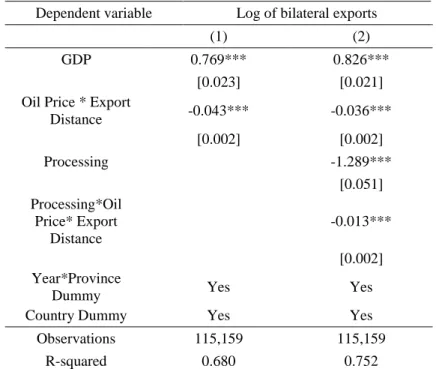
(21) 5. Regression Results The results from the estimation of equations (1), (2) and (3) are presented in Tables 4 and 5. The log of Chinese provincial exports is our dependent variable and each specification includes province-time fixed effects and country fixed effects (not reported because of space constraints). To account for zeros, all coefficients are estimated using the two-stage procedure developed by Helpman et al. (2008). In all equations we compute standard errors that are robust to clustered heteroscedasticity (White, 1980). Column (1) of Table 4 reports coefficient estimates without controlling for the type of trade. The coefficient on oil price*export distance is negative and significant, providing support for Hypothesis 1. In other words, a rise in oil prices increases the sensitivity of China‘s exports to distance. In column (2) of Table 4, we interact the dummy regime with oil price*export distance to test whether oil prices affect trade‘s sensitivity to distance differently depending on the type of trade. We find that the coefficients on both oil price*export distance and regime*oil price*export distance are negative and significant, suggesting that a rise in oil prices increases the sensitivity of China‘s processing exports to distance more than for non-processing exports. [Table 4 about here]. In Table 5, we interact the dummy variable air with oil price*export distance to test whether oil prices affect trade‘s sensitivity to distance differently depending on the mode of transport. Column (1) shows the coefficient estimates when our sample is pooled across both processing and non-processing exports, while columns (2) and (3) show the. 18.
(22) results for processing and non-processing exports, respectively. The results are in line with hypothesis 3. In all three columns, the coefficient on oil price*export distance is negative and significant, while the coefficient on air*oil price*export distance is positive and significant. This suggests that a rise in oil prices makes China‘s exports more sensitive to distance, but less so for trade by air.. [Table 5 about here]. How large are these effects? One way to assess this is to consider the implied increase in distance effects for the oil price changes that have occurred in recent years. At the roughly US$26 per barrel price of 2002, the combined coefficient on log distance in Table 4 column (1) is approximately -0.043*ln(26) = -0.14. After nearly quadrupling to about US$100 in 2008, the combined coefficient is roughly -0.043*ln(100) = -0.20. This suggests that the dramatic oil price rise between 2002 and 2008 has increased the distance elasticity of exports by 0.06 percentage points. Distance coefficients from similar gravity models typically range from 0.9 to 1.1 (Disdier and Head, 2008), so that our result would suggest an increase in distance elasticity of about 5.5-6.7%. These strike us as relatively small, challenging Rubin and Tal‘s (2008) argument that rising oil prices will make trade substantially more sensitive to distance. In Table 6, we estimate the differential impact of a hypothetical increase in oil prices from US$26 to US$100 depending on the type of trade (processing versus nonprocessing) and the mode of transport (air-intensive versus non-air-intensive). The appendix presents the complete calculation. Using the estimated coefficients in columns (2) and (3) of Table 5, the oil price increase would have a negligible impact on the. 19.
(23) sensitivity of air-intensive exports to distance. In air-intensive industries, the distance elasticity would in absolute value rise by 0.02 and 0.03 percentage points for processing and non-processing exports, respectively. In non-air-intensive industries, the effect is larger. For processing exports, the distance elasticity would in absolute value rise by 0.13 percentage points, while for non-processing exports it would increase by 0.09 percentage points. This would correspond to an increase in the distance elasticity of approximately 10% for non-air-intensive trade.. [Table 6 about here] The relatively small impact of oil price changes on trade‘s elasticity to distance should not be entirely surprising to international business scholars. An influential literature in international business has highlighted that international business strategy is regional rather than global, and that this is largely due to factors other than transportation costs (Ghemawat, 2003; Buckley and Ghauri, 2004; Ricart et al., 2004; Rugman and Verbeke, 2004, 2007). In conclusion, we find evidence supporting the hypothesis that China‘s exports have become more sensitive to distance in times of rising oil prices. The size of the impact, however, depends on the type of trade and the mode of transport. Processing exports have seen a larger increase in their sensitivity to distance during times of rising oil prices than non-processing exports. Conversely, exports in air-intensive industries have seen a smaller increase in their sensitivity to distance during times of rising oil prices than exports in ocean-intensive industries. While these results are statistically significant, their economic effects are relatively small. Our analysis therefore finds that concerns of. 20.
(24) business analysts that rising oil prices will increase substantially trade‘s sensitivity to distance are likely overblown.. 6. Discussion and Concluding Remarks In this paper, we have taken up the question of whether higher oil prices may mean a substantial reduction in global trade, particularly within global production networks. Using a unique dataset of Chinese trade, which distinguishes between processing and other trade, we estimate variants of the gravity model of trade that incorporate oil price effects. We find that there is a significant effect of oil prices on the relationship between exports and distance: higher oil prices make distance a bigger barrier to trade. As expected, these effects are larger for processing trade than for non-processing trade, since vertically specialized trade requires goods to cross borders multiple times. In addition, we find that exports shipped by air are less sensitive to oil prices than exports shipped by ocean, consistent with their higher weight-to-value ratio and their greater dependence on considerations such as timeliness that may outweigh transport costs. That oil prices matter is not surprising. Perhaps the more important question is what the magnitudes of these effects are. We find effects that appear small, although it is harder to make an intuitive judgment as to whether these might be viewed by firms as qualitatively important. Our estimates suggest that the quadrupling of oil prices from an annual average of US$26 in 2002 to nearly US$100 a barrel in 2008 would increase trade‘s elasticity to distance by a mere 5.5-6.7%. There are important limitations to this study that arise from the nature of the available data and the empirical specification that we have employed. The limited variability of oil. 21.
(25) prices over the 1988-2008 period—they were largely flat in real terms for the first half of the sample before surging upward—means that it may be difficult to precisely estimate oil price effects. Another limitation of our analysis is that it may be difficult to separate the influence of oil prices from other time-varying factors that may have trended upward in the early twenty first century. For example, if over the past decade the adoption of justin-time production techniques has become more pronounced, this may have led firms to source products from nearby countries, regardless of changes in transportation costs (Evans and Harrigan, 2005). Our analysis partially controls for this by making distinctions between types of trade and modes of transport, but more work needs to be done to further disentangle these effects. Finally, our specification imposes constant elasticities of the distance effect with respect to oil prices.. This may not be an. appropriate assumption. Hummels (2007), for example, notes that the gains from air transport are larger for long distances than for shorter ones. This suggests that the impact of higher oil prices may not alter export behavior in a linear fashion. It seems unlikely that the dire predictions of the ―end of globalization‖ will come to pass, at least assuming that oil prices rise only moderately from current high levels, as expected by most forecasting agencies. Differences in factor endowments remain very large, and technological change will provide ways to offset some of the future cost increases.. But it is nevertheless likely that the expansion of global trade will be. restrained by high energy costs, compared with its rapid expansion in recent decades. Considering the paucity of existing literature, this should be a fruitful area for research in coming years.. 22.
(26) Bibliography Adams, G. (2009). Will economic recovery drive up world oil prices? World Economics 10(2): 1-26. Anderson, J. Forthcoming. The gravity model. Annual Review of Economics 3. Anderson, J., and E. van Wincoop. 2003. Gravity with gravitas: a solution to the border puzzle. American Economic Review 93(1): 170-192. Anderson, J., and E. van Wincoop. 2004. Trade costs. Journal of Economic Literature 42(3): 691-751. Athukorala, P., and N. Yamashita. 2006. Production fragmentation and trade integration. North American Journal of Economics and Finance 17(3): 233-256. Baier, S., and J. Bergstrand. 2001. The growth of world trade: tariffs, transport costs, and income similarity. Journal of International Economics 53(1): 1–27. Buckley, P. and P. Ghauri. 2004. Globalization, economic geography and the strategy of multinational enterprises. Journal of International Business Studies 35(2): 81-98. De Almeida, P., and P. Silva. 2009. The peak oil production – timings and market recognition. Energy Policy 37(4): 1267-1276. Disdier, A.-C., and K. Head. 2008. The puzzling persistence of the distance effect on bilateral trade. Review of Economics and Statistics 90(1): 37-48. Economist. 2008. High seas, high prices. How much will rising shipping costs hurt Chinese manufacturing? August 7th. Egger, P. 2008. On the role of distance for bilateral trade. The World Economy 31(5): 653-662. Evans, C., and J. Harrigan. 2005. Distance, time, and specialization: Lean retailing in general equilibrium. American Economic Review 95(1): 292-313. Faruqee H. 2004. Measuring the trade effects of EMU. IMF Working Paper No. 04/154. Feenstra, R. 2004. Advanced International Trade: Theory and Evidence. Princeton: Princeton University Press. Feenstra, R., H. Deng, A. Ma, and S. Yao. 2004. Chinese and Hong Kong international trade data. Mimeo. Fidrmuc, J. 2009. Gravity models in integrated panels. Empirical Economics 37(2): 435446. Fratianni, M., F. Marchionne, and C. Oh. Forthcoming. A commentary on the gravity equation in international business research. Multinational Business Review. Gangnes, B., and A. Van Assche. 2010. China and the future of Asian technology trade. In The Future of Asian Trade and Growth: Economic Development with the Emergence of China,ed. L. Yueh, 351-377. London: Routledge. 23.
(27) Gengenbach, C. 2009. A panel cointegration study of the Euro effect on trade. Maastricht University mimeo. Ghemawat, P. 2003. Semiglobalization and international business strategy. Journal of International Business Studies 34(2): 138-152. Grossman, G., and E. Rossi-Hansberg. 2008. Trading tasks: A simple theory of offshoring. American Economic Review 98(5): 1978-1997. Haddad, M. 2007. Trade integration in East Asia: The role of China and production networks. World Bank Policy Research Working Paper 4160. Harrigan, J. 2010. Airplanes and comparative advantage. Journal of International Economics 82(2): 181-194. Hatzichronoglou, T. 1997. Revision of the high-technology sector and product classification. OECD Science, Technology and Industry Working Papers, 1997/2. Helpman, E., M. Melitz, and Y. Rubinstein. 2008. Estimating trade flows: Trading partners and trading volumes. Quarterly Journal of Economics 123(2): 441-487. Hummels, D. 2007. Transportation costs and international trade in the second era of globalization. Journal of Economic Perspectives 21(3): 131-154. Hummels, D., I. Ishii, and K.-M. Yi. 2001. The nature and growth of vertical specialization in world trade. Journal of International Economics 54(1): 75-96. Hummels, D., and G. Schaur. 2010. Hedging price volatility using fast transport. Journal of International Economics 82(1): 15-25. Jen, S., and L. Bindelli. 2008. High transport costs to ‗un-flatten‘ the world. Morgan Stanley Research. Koopman, R., Z. Wang, and S.-J. Wei. 2008. How much of Chinese exports is really made in China? Assessing domestic value-added when processing trade is pervasive. NBER Working Paper 14109. Lin, S. 2005. International trade, location and wage inequality in China. In Spatial inequality and development, eds. R. Kanbur and A. Venables, 260-292. Oxford: Oxford University Press. Linden, G., K. Kraemer, and J. Dedrick. 2009. Who captures value in a global innovation network? The case of Apple‘s iPod. Communications of the ACM 52(3): 140-144. Limao, N., and A. Venables. 2001. Infrastructure, geographical disadvantage, transport costs, and trade. The World Bank Economic Review 15(3): 451-79. Ma, A., and A. Van Assche. 2010. The role of trade costs in global production networks: Evidence from China‘s processing trade regime. World Bank Policy Research Working Paper No. 5490.. 24.
(28) Ma, A., and A. Van Assche. Forthcoming. China‘s role in global production networks. In Trade Policy Research Special Edition: Global Value Chains – Impacts and Implications, ed. A. Sydor. Ottawa: Department of Foreign Affairs and International Trade. Ma, A., A. Van Assche, and C. Hong. 2009. Global production networks and China‘s processing trade. Journal of Asian Economics, 20(6): 640-654. Miroudot, S., and A. Ragoussis. 2009. Vertical trade, trade costs and FDI. OECD Trade Policy Working Paper No. 89. Mirza, D., and H. Zitouna. 2009. Oil prices, geography and endogenous regionalism: too much ado about (almost) nothing. CEPII Working Paper No. 2009-26. Murphy, S. 2008. Will sourcing come closer to home? Supply Chain Management Review (September): 33-37. Radelet, S., and J. Sachs. 1998. Shipping costs, manufactured exports, and economic growth. Columbia University Earth Institute, mimeo. Ricart, J., M. Enright, P. Ghemawat, S. Hart, and T. Khanna. 2004. New frontiers in international strategy. Journal of International Business Studies 35(1), 175-200. Rubin, J. 2009. Why your world is going to get a whole lot smaller: oil and the end of globalization. Toronto: Random House. Rubin, J., and B. Tal. 2008. Will soaring transport costs reverse globalization? CIBC World Markets StrategEcon (May): 4-7. Rugman, A. and A. Verbeke. 2004. A perspective on regional and global strategies of multinational enterprises. Journal of International Business Studies 35(1): 3-19. Rugman, A. and A. Verbeke. 2007. Liability of regional foreignness and the use of firmlevel versus country-level data: A response to Dunning et al. (2007). Journal of International Business Studies 38(1), 200-205. Santos-Silva, J., and S. Tenreyro. 2006. The log of gravity. Review of Economics and Statistics 88(4): 641-658. Sturgeon, T. 2002. Modular production networks: a new American model of industrial organization. Industrial and Corporate Change 11(3): 451–496. UNCTAD. 2010. Oil prices and maritime freight rates: an empirical investigation. Technical Report. US Energy Information Agency. 2010. Annual Energy Outlook 2010. White, H. (1980). A heteroskedasticity-consistent covariance matrix estimator and a direct test for heteroskedasticity. Econometrica 48(4): 817-838. Yi, K.-M. 2003. Can vertical specialization explain the growth of world trade? Journal of Political Economy 111(1): 52-102.. 25.
(29) Appendix In this appendix, we calculate the impact of a hypothetical increase in oil prices from US$26 to US$100 on the elasticity of Chinese exports to distance, by type of trade (processing versus non-processing) and mode of transportation (air-intensive versus seaintensive). We report these results in Table 6. First, we use the estimated coefficients in column (2) of Table 5 to measure the impact of the oil price increase on non-air-intensive processing exports. Since the dummy variable air equals 0 for non-air-intensive exports, the combined coefficient on log distance at an oil price of US$26 is -0.094*ln(26)+0*0.079*ln(26)= -0.30. At US$100, the combined coefficient changes to -0.094*ln(100)+0*0.079*ln(100)= -0.43. This suggests that an oil price surge from US$26 to US$100 increases the distance elasticity of non-air-intensive processing exports by 0.13 percentage points. Next, we use the estimated coefficients in column (2) of Table 5 to measure the impact of the oil price rise on the distance elasticity of air-intensive processing exports. In this case, the dummy variable air equals to 1. As a result, the combined coefficient on log distance at an oil price of US$26 is -0.094*ln(26) + 1*0.079*ln(26) = -0.05. At US$100, the combined coefficient changes to -0.094*ln(100) + 1*0.079*ln(100) = -0.07. This implies that an oil price increase from US$26 to US$100 increases the distance elasticity of airintensive processing exports by 0.02 percentage points. By using the coefficients in column (3) of Table 5 and the same steps as above, it is straightforward to also measure the impact on non-air-intensive ordinary exports and airintensive ordinary exports.. 26.
(30) Figure 1: Average real crude oil prices, 2009US$/barrel, 1980-2010 120. 100. 80. 60. 40. 20. 0. Source: Authors calculations based on data from Federal Reserve Bank of St. Louis and US Bureau of Labor Statistics. Oil price is the spot price of West Texas Intermediate crude. Final observation is approximate monthly value for December 2010.. 27.
(31) Figure 2: regular trade versus vertically specialized trade. Vertically specialized trade. Regular trade. Input. Country 1. Input Final good. Country 2 Final good. Country 3. Consumer. Consumer. 28.
(32) Figure 3: Proportion of processing trade in China’s total trade, 1988-2008 60. Percentage. 50 40 30 20 10 0 1988. 1990. 1992. 1994. 1996. 1998. 2000. 2002. Year Export. Import. Source: Authors‘ calculations using China‘s Customs Statistics.. 29. 2004. 2006.
(33) Figure 4: Domestic and foreign content share of China’s processing and nonprocessing exports Non-Processing Exports. Processing Exports. Foreign content share: 11%. Chinese content share: 18%. Foreign content share: 82%. Chinese content share: 89%. Source: Koopman et al. (2008).. 30.
(34) Figure 5: Share of China’s exports conducted by foreign-invested enterprises, 19882008 100 90 80 70 60 50 40 30 20 10 0. processing exports. non-processing exports. Source: authors‘ calculations, using China‘s Customs Statistics.. 31.
(35) Figure 6: Share of processing exports in China’s total exports, by technology level (%), 1992-2008. 100 90 80 70 60 50 40 30 20 1992. 1994. 1996 1998 High-tech. 2000. Medium-low tech. 2002 2004 2006 Medium-high tech. Low-tech. Source: authors‘ calculations, using China‘s Customs Statistics. 32. 2008.
(36) Figure 7: Share of exports in air-intensive industries (%), by customs regime, 1988-2008 80 70 60 50 40 30 20 10 0. Processing exports. Non-processing exports. 33.
(37) Table 1. Projections of World Real Oil Prices (2008 US$ per barrel), 2015-2035 2015. 2020. 2025. 2030. 2035. USEIA 2010 (Reference). 94.52. 108.28. 115.09. 123.50. 133.32. INFORUM. 92.50. 107.98. 109.74. 116.81. --. DB. 93.18. 105.48. 114.65. 121.16. 125.42. IHSGI. 85.07. 81.93. 74.86. 77.27. 80.03. --. 100.00. --. 115.00. --. EVA. 80.35. 84.45. 90.98. 100.43. --. SEER (Business as Usual). 79.20. 74.31. 69.73. 65.43. --. SEER (Multi-Dimensional). 99.03. 101.52. 105.81. 113.91. --. IEA (Reference). Source: "Comparison with other projections", from Annual Energy Outlook 2010, US Energy Information Agency. Organizations listed are Interindustry Forecasting Project at the University of Maryland (INFORUM), Deutsche Bank (DB), IHS Global Insight (IHSGI), the International Energy Agency (IEA), Energy Ventures Analysis, Inc. (EVA), and Strategic Energy & Economic Research, Inc. (SEER).. 34.
(38) Table 2. Proportion of exports shipped by air, major exporting industries. 1988. 1998. 2008. Exports by air, % of total 2009. 4.10. 22.56. 33.50. 33.84. 3.00. 12.69. 28.04. 33.03. 0.42. 3.40. 3.96. 29.83. 3.73. 0.54. 1.01. 11.78. Share of total exports. HS2 code. 29. Electrical machinery & equipment & parts, telecommunications equipment, sound recorders, television recorders Nuclear reactors, boilers, machinery & mechanical appliances, computers Optical, photographic, cinematographic, measuring, checking, precision, medical or surgical instruments & accessories Organic chemicals. 62. Articles of apparel & clothing accessories – not knitted or crocheted. 18.62. 8.33. 2.54. 9.62. 61. Articles of apparel & clothing accessories, knitted and crocheted. 2.47. 4.02. 1.15. 7.44. 39. Plastics & articles thereof. 1.55. 3.77. 2.64. 1.99. 87. Vehicles other and railway or tramway rolling stock. 0.71. 1.34. 1.80. 1.35. 64. Footwear, gaiters and the like. 3.63. 5.63. 1.79. 1.12. 40. Rubbers & articles thereof Railway or tramway locomotives, rolling stock, track fixtures & fittings, signals Toys, games and sports equipment, parts & accessories Furniture, bedding, cushions, lamps & lighting fittings nesoi, illuminated signs, nameplates & the like, prefabricated buildings Ships, boats, & floating structures. 2.03. 0.73. 1.94. 0.97. 0.01. 1.67. 1.36. 0.88. 2.46. 5.96. 2.60. 0.81. 1.51. 2.27. 2.06. 0.65. 1.44. 1.74. 3.13. 0.01. 85 84 90. 86 95 94 89. Authors‘ calculations using China‘s Customs Statistics Data. 35.
(39) Table 3. Descriptive Statistics and Data Sources Mean Exports (US$ million). (1). 13.485. Std. Dev. 2.861. Min.. Max.. 0.693. 24.395. China Customs Statistics. Oil Price (US$/barrel). (2). 3.365. 0.559. 2.644. 4.585. International Financial Statistics. GDP (US$). (3). 24.412. 2.233. 17.162. 30.285. World Economic Outlook. Export Distance (km). (4). 8.458. 0.666. 4.236. 9.413. Lin (2005). Processing. (5). 0.358. 0.479. 0.000. 1.000. China Customs Statistics. Air. (6). 0.415. 0.493. 0.000. 1.000. China Customs Statistics. Note: Other than dummies, all variables are in natural logarithms.. 36. Data source.
(40) Table 4. Panel regressions: effect of oil prices on export sensitivity to distance, total and processing trade Regression results, 1988-2008 Dependent variable GDP Oil Price * Export Distance. Log of bilateral exports (1). (2). 0.769***. 0.826***. [0.023]. [0.021]. -0.043***. -0.036***. [0.002]. [0.002]. Processing. -1.289*** [0.051]. Processing*Oil Price* Export Distance. -0.013*** [0.002]. Year*Province Dummy Country Dummy Observations. Yes. Yes. Yes. Yes. 115,159. 115,159. R-squared 0.680 0.752 Notes: Robust standard errors are in parentheses. * means significant at 10%; ** means significant at 5%; *** means significant at 1%. Coefficients on constant term, on fixed effects and on the first stage not reported. Other than dummies, all variables are in natural logarithms.. 37.
(41) Table 5. Panel regressions: effect of oil prices on export sensitivity to distance, shipments by air and by surface transport Regression results, 1988-2008 Log of bilateral total exports (1). Log of bilateral processing exports (2). Log of bilateral ordinary exports (3). GDP. 0.719***. 0.732***. 0.786***. [0.018]. [0.030]. [0.021]. Oil Price * Export Distance. -0.075***. -0.094***. -0.064***. [0.002]. [0.003]. [0.002]. Air. -2.815***. -3.100***. -2.979***. [0.045]. [0.073]. [0.049]. Air*Oil Price* Export Distance. 0.049***. 0.079***. 0.037***. Year*Province Dummy Country Dummy. [0.002] Yes Yes. [0.003] Yes Yes. [0.002] Yes Yes. Observations. 190,579. 68,689. 121,890. R-squared 0.645 0.677 0.744 Notes: Robust standard errors are in parentheses. * means significant at 10%; ** means significant at 5%; *** means significant at 1%. Coefficients on constant term and on fixed effects not reported. Other than dummies, all variables are in natural logarithms.. 38.
(42) Table 6. Percentage point change in the elasticity of exports to distance if oil prices rises from US$26 to US$100, by type of trade and transport mode. Air-intensive exports Non-air intensive exports. Processing exports -0.02 -0.13. Source: Authors‘ calculations. 39. Non-processing exports -0.04 -0.09.
(43) End Notes 1. Rubin (2009) expanded on this argument in his award-winning book Why Your World Is Going to Get a Whole Lot Smaller: Oil and the End of Globalization. The title of our paper refers to this book. 2 Existing research on the effects of overall transportation costs on trade volume does not provide a clear result, perhaps because of a wide variety of empirical approaches and specifications. Some papers appear to find large effects of transport costs on trade. Limao and Venables (2001) find that a doubling of transport costs would reduce trade by 45%. Radelet and Sachs (1998) conclude that an increase in the CIF/FOB band from 12% to 17% would reduce the long-term annual growth rate of non-primary manufactured exports by 0.2 percentage points of GDP. On the other hand, Baier and Bergstrand (2001) find that transportation cost changes explain only 8% of the growth in world trade in the post-World War II period. And Rose (1991) does not find that transportation costs have a statistically significant effect on global trade growth in the 1951-81 period. 3 Grossman and Rossi-Hansberg (2008) have eloquently described this a shift from trade in goods to trade in tasks. 4 In principle one could directly assess the effect of the value-to-weight ratio and utility value of timely delivery on the sensitivity of trade to oil price changes, but reliable data are difficult to come by. 5 In order to estimate the ultimate destination country of Chinese exports that are re-exported through Hong Kong, we link the Chinese trade data to a data set from the Hong Kong Census and Statistical Office on Hong Kong re-exports. See Ma et al. (2009) for more details. 6 As Ma and Van Assche (2010) explain, the data set on China‘s processing trade regime is one of only a few data sources that allow us to gain insights into the nature of vertically specialized trade. 7 Foreign-invested enterprises include wholly foreign-owned enterprises, Sino-foreign contractual joint ventures with more than 25% foreign ownership, and Sino-foreign equity joint ventures with more than 25% foreign ownership. Note that in China‘s Customs Statistics, companies from Hong Kong, Macau and Taiwan are considered foreign firms. 8 High-technology industries include aerospace, pharmaceuticals, office and computing machinery, radio, TV and communication equipment and medical, precision and optical instruments. 9 We broadly define electronics as the HS 2-digit codes 84, 85 and 90. 10 We only have access to data on the mode of transportation for the year 2009. 11 See Fratianni et al. (forthcoming) for a discussion of the gravity equation in international business research. 12 The multilateral resistance term takes into account that bilateral trade flows not only depend on the bilateral trade costs between the home and host country, but also on the average trade costs across all other countries. 13 We do not include country-time fixed effects since this would not allow us to estimate the impact of oil price changes on trade‘s sensitivity to distance. 14 Our specification also does not include bilateral variables such as common colony, common border and common language. These variables do not vary across Chinese provinces, thus making them countryspecific. 15 The estimation results may be affected by the potential non-stationarity of some variables. Although spurious regression problems are of less concern in panel settings than in standard time-series analysis, because the fixed effects estimator for non-stationary data is asymptotically normal, there will be bias in small samples (Fidrmuc, 2009; Kao and Chiang, 2000). There remain very few papers that analyze the effect of non-stationarity in panel gravity model settings, including Faruqee (2004) and Gengenbach (2009). On the basis of Monte Carlo analysis, Fidrmuc (2009) concludes that the potential bias from use of fixed effects models appears to be relatively small. 16 Similar to Helpman et al. (2008), the first-stage regression includes province, country, and year fixed effects. To ensure that we do not need to rely on the normality assumption for the unobserved trade costs, we also include the following excluded variable: a dummy that equals to 1 if both the province and the country have a coast. Step 1 regressions are not reported here.. 40.
(44)
Figure
+7
Documents relatifs
Although the extent of preferential access for apparel to the US market provided by AGOA is similar (measured by an average US MFN tariff of 11.5% in 2004) to the one provided by
returning wallets untouched to pedestrians. offering his scarf to keep
In the general case we can use the sharper asymptotic estimate for the correlation kernel corresponding to a real analytic potential from the proof of Lemma 4.4 of [4] (or Theorem
This allows us to give the asymptotic distribution of the number of (neutral) mutations in the partial tree.. This is a first step to study the asymptotic distribution of a
The EU’s trade policy response to the corona crisis has so far been in line with the reaction to the euro crisis: export restrictions should be limited and temporary,
Since 2001, under the US Africa Growth Opportunity Act (AGOA), 22 African countries exporting apparel to the US can use fabric from any origin and still meet the criterion
R´ esum´ e (La dimension de Kodaira des vari´ et´ es de Kummer). — Nous montrons que les vari´et´ es de Kummer T /G de dimension 3 et de dimension alg´ebrique 0 sont de dimension
The identification of population groups that will benefit most from diagnosis and treatment of LTBI should be based on the evidence of increased prevalence of LTBI, increased risk
