Development of bed configurations in coarse sands.

-~ U

DEVELOPMENT OF BED CONFIGURATIONS IN COARSE SANDS

by

Warren Russell Costello

B.Sc. (1968), M.Sc. (1970) McMaster University

SUBMITTED IN PARTIAL FULFILLMENT OF THE REQUIREMENTS FOR THE DEGREE OF DOCTOR OF PHILOSOPHY

at the

Massachusetts Institute of Technology January, 1974 Signature of Author . Certified by A Accepted by C- * * '*~-,--' ~. Thepis Supervisor

Chairman, Departmental Committee on Graduate Studies

Archives

(\NOV 5 1974

ABSTRACT

Development of Bed Configurations in Coarse Sands by

Warren Russell Costello

Submitted to the Department of Earth and Planetary Sciences in partial fulfillment of the requirement for the

degree of Doctor of Philosophy

Flume experiments were conducted with five coarse sands of different sizes to investigate the development of bed configurations. For fixed depth and increasing velocity, the bed configurations are no movement, flat bed, ripples, bars, and dunes. For sand sizes coarser than about 0.70 mm, ripples are replaced by a flat bed. By introducing an ir-regularity on the sediment bed, ripples can be initiated in the no-movement and flat-bed phases.

Ripples develop because of the effect of turbulence on the bed in the reattachment zone. The resulting strong instantaneous shear stresses initiate a maximum in sediment transport, which generates a ripple. Bars, a newly defined bed configuration, form because of the merging of kinematic waves of bed height and sediment transport to form a kine-matic shock wave. At higher velocities flow acceleration

over the bars is strong enough to affect the bed downstream of reattachment so that a maximum in mean shear stress and sediment transport is established; this initiates dune devel-opment.

The sequence ripples++-bars++dunes observed in the ex-periments matches that observed in rivers and in the ocean. Sand waves and transverse bars in natural environments are large-scale bars with similar mechanics and occupying the same stabiltiy field as the experimental bars reported here. Thesis Supervisor: John B. Southard

TABLE OF CONTENTS ABSTRACT ₂ TABLE OF CONTENTS 3 LIST OF SYMBOLS ₆ LIST OF FIGURES ₉ LIST OF TABLES ₁₂ ACKNOWLEDGMENTS 13 1. INTRODUCTION 14 INTRODUCTORY NOTE 14 HISTORICAL BACKGROUND 15

PURPOSE AND OUTLINE 25

2. EXPERIMENTAL APPARATUS AND PROCEDURE 27

APPARATUS 27

5.5 m Flume 27

11.5 m Flume 30

Sediment Discharge Measurement 35

Velocity Profile Measurement 35

SANDS 36

Source 36

Sediment Analysis 37

EXPERIMENTAL PROCEDURE 37

3. PRESENTATION AND DISCUSSION OF EXPERIMENTAL RESULTS 48

BASIC DATA 48

General 48

Reproducibility and Equilibrium 48

Terminology 55

Observations 58

Hydraulic Data 68

Geometrical Proporties of Bed Forms 73

BED PHASES 81

1.14 mm Sand 81

0.51 mm-0.80 mm Sands ₈₃

Discussion of Phase Relations 85

4. MECHANICS OF BED FORMS 98

RIPPLES 98

Inglis-Raudkivi Model 99

Flow Separation over a Negative Step 100 Development of Initial Bed Disturbance 104

Ripple Model ₁₀₇

BARS ₁₂₀

Kinematic Wave Theory 121

Previous Theory ₁₂₆ Bar Movement 129 DUNES ₁₃₅ Kennedy Model 136 Velikanov-Mikhailova-Yalin Model 137 Mechanics of Dunes 140

Flow Separation and Reattachment 146

Dune Model ₁₅₃

CONCLUSION ₁₆₀

5. FIELD OBSERVATIONS OF BED CONFIGURATIONS 162

5

Comparison of Flume and Field Observations 169

Discussion 174

TRANSVERSE BARS IN RIVERS 179

Comparison of Experimental Bars and Transverse

Bars 182 CONCLUSIONS 185 6. SUMMARY OF CONCLUSIONS 187 REFERENCES 191 APPENDIX A 204 BIOGRAPHY 206

6

LIST OF SYMBOLS

a porosity of sediment

A cross-sectional area of flow A bed wave amplitude

b width of channel

c slope of the sediment transport rate versus bed height curve

C₁ constant of discharge in equation 6, Chapter 4

C2 empirical coefficient in sediment discharge equation

C_{3 constant in equation 8, Chapter 4, C}

3 = C 1 C2

d depth of flow

D geometric mean sieve size of bed load

f Darcy-Weisbach friction factor, f = 8 (V,/U)2

f b bed friction factor, fb = 8(V /U)2 l2b F Froude number, F = U/(gd)1

g acceleration due to gravity

gs sediment discharge per unit width h height of individual bed form or step

h9 0distance from water surface to some arbitrary datum h u height of next individual bed form upstream

j

j

k. length of individual bed forms L length of sediment wave

Q mean flow discharge

P wetted perimeter of channel r hydraulic radius, r = A/P

rb bed hydraulic radius, rb = rfb/f R flow Reynolds number, R = 4Ur/v

R* boundary Reynolds number, R* = V*D /v S energy slope ( water surface slope)

t time

T water temperature

u instantaneous streamwise flow velocity U mean flow velocity

U mean velocity for threshold of particle motion Um maximum velocity in a vertical section in flow v instantaneous spanwise flow velocity

V* shear velocity, V* = (grS)1/2

V* bed shear velocity, V* = (grbS)1/2

b b

x longitudinal coordinate along bed downstream y vertical coordinate, upward from bed

y+ dimensionless distance above bed, y+ = y (T 1/2 a attentuation factor in autocorrelation function y specific weight of fluid, y = pg

YS specific weight of sediment, ys = Psg

6 distance local sediment transport lags behind local velocity

dynamic fluid viscosity v kinematic fluid viscosity

p density of fluid ps density of sediment

a geometric standard deviation of sediment size 9

T mean shear stress at bed Shields parameter, T*=T

LIST OF FIGURES Fig. Fig. Fig. Fig. Fig. Fig. Fig. Fig. Fig. Fig. Fig. Fig. Fig. Fig. 2.1 2.2 2.3 2.4a 2.4b 2.4c 2.4d 2.4e 3.1 3.2 3.3 3.4 3.5 3.6 Fig. 3.7 Fig. 3.8

Schematic diagram of 5.5 m flume. Schematic diagram of 11.5 m flume.

Distribution of grain sizes of the sands used in series A-E.

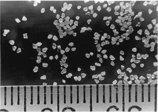
Photograph of sample of 0.51 mm sand (series A). Photograph of sample of 0.60 mm sand (series B). Photograph of sample of 0.66 mm sand (series C). Photograph of sample of 0.80 mm sand (series D). Photograph of sample of 1.14 mm sand (series E). Development of a ripple train from a line

disturbance on a flat bed with no grain motion. Newly formed ripples in the flat bed (meta-stable ripple) phase.

Upstream view of rippled bed surface. Migration of small waves on a flat bed.

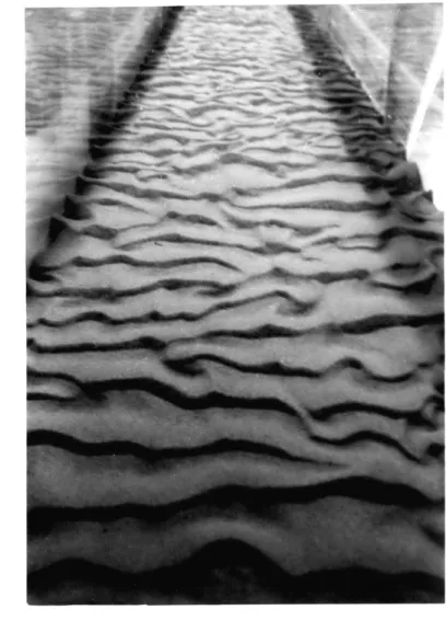
Large, fully developed bars stretching across the width of the flume.

View upstream of fully developed dunes with three-dimensional geometry and ripples on the stoss slopes.

Variation of energy slope and bed friction factor with changes in mean velocity.

Variation of sediment transport rate with changes in mean velocity.

28 31 38 39 39 40 40 41 60 61 63 64 66 67 69 Page

10 Fig. Fig. Fig. Fig. Fig. Fig. Fig. Fig. Fig. Fig. Fig. Fig. Fig. Fig. Fig. 3.9 3.10 3.11 3.12 3.13 3.14 3.15 3.16 4.1 4.2 4.3 4.4 4.5 4.6 4.7 Fig. 4.8 Fig. 4.9

Histograms of ripple, bar and dune lengths. Histograms of ripple, bar and dune heights. Histograms of length/height ratios for

ripples, bars and dunes.

Depth-velocity diagram for 1.14 mm sand.

Depth-velocity diagram for sands in series A-D. Comparison of grain motion with the Shields criterion.

Erosive lineations on a hummocky bed surface. Pathlines of bars in space and time.

Velocity and turbulence measurements down-stream of a negative step.

Length of reverse flow region downstream of a negative step.

Idealized model of ripple development. Histograms of ripple length/ripple height and ripple length/upstream ripple height. Development of a kinematic shock wave. Pathlines of bars and ripples in space and time.

Idealized effect of sediment transport rate maximum.

Depth-velocity diagram for measurements of a maximum in sediment transport downstream of a negative step.

Shear stress maximum for reattaching flows.

74 76 79 82 84 87 89 93 102 103 112 117 123 133 142 144 150

Fig. 4.10 Fig. Fig. Fig. 5.1 5.2 5.3 Fig. 5.4 Fig. 5.5 Fig. 5.6

Histograms of dune length/dune height and dune length/upstream dune height.

Ebb-oriented dunes on a complex flood-oriented sand wave, Minas Basin.

Depth-velocity diagram for 0.49 mm sand.

Depth-velocity diagram for the bed configura-tions in the Parker River Estuary.

Hypothetical time pathline of depth and velocity through a flood tide.

Time history of depth and velocity over ebb and flood tides in the Minas Basin.

Idealized time history of depth and velocity through a river flood cycle.

155 168 171 172 176 177 184

LIST OF TABLES Table 2.1 Table 3.1 Table 3.2 Table 3.3 Table 3.4 Table 3.5

Physical Characteristics of Sands Summary of data, 11.5 m flume Summary of data, 11.5 m flume Summary of data, 5.5 m flume

Reproducibility of experimental runs Data on initiation of movement

Page 42 49 51 53 54 86

13

ACKNOWLEDGMENTS

I wish to thank Professor John B. Southard for his guidance and support throughout this study. Without his valuable suggestions and criticisms this work would not have been completed. I also wish to thank Jon Booth-royd for the loan of his excellent field data on sand waves. My fellow students Wilford Gardner, Lawrence

Boguchwal, Mary Jane Goettal and Robert Young have provided many hours of fruitful discussion and have helped to make

life at M.I.T. more enjoyable.

Finally I offer my deepest appreciation to my wife, Susan, who was my typist, sand siever, draftswoman, and editor, for her patience and understanding.

This work was supported by the Office of Naval Research under contract N 00014-67-A-0204-0048.

-~ I

1. INTRODUCTION

INTRODUCTORY NOTE

Sediment transported by water has an appreciable effect on the flow. High concentrations of suspended

sediment alter the momentum exchange and hence the tur-bulence structure, while sediment transported along the bed alters flow depth and energy loss due to changes in channel geometry and roughness. In addition to the effect of transported sediment on the fundamental flow laws, knowledge of the capacity of a flow to transport sediment has economic relevance with respect to erosion, flood control, navigation, irrigation, pollution, and harbor maintenance.

In addition to these engineering applications, sediment transport is of primary interest to geologists who interpret modern and ancient sediments deposited by rivers, lakes, and the ocean. A ubiquitous characteristic of these sediments is cross-stratification, which seems to be largely the result of sediment being transported on

the bed as migrating grain mounds. In the last two decades the study of these bed forms has increased greatly, first in an attempt to discern direction of transport in ancient environments, and, more recently, in an attempt to charac-terize the hydraulic setting in the ancient flow system.

Mw

15

sediment transport have only been partially outlined. The result has been great uncertainty as to how well sediment transport can be predicted, even irrespective of what form the bed-load movement will assume. Without

full knowledge of the mechanics of bed-form movement, engineers and geologists have had to resort to empirical classifications in attempts at prediction and interpreta-tion. Out of this empirical approach has emerged the concept of a definite sequence of bed configurations; this concept has managed to put into some order a vast amount of empirical observation.

If the mechanics of development of different bed configurations can be accurately deduced, scientists will have an effective tool for prediction in modern sediment transport and for interpretation in ancient sedimentary deposits. Many theories have been put forward to explain this complex phenomenon. In the following section a brief historical summary outlines the main contributions.

HISTORICAL BACKGROUND

Flow-produced bed forms have been the subject of investigation by geologists and hydraulicians since the nineteenth century. It was Sorby who first interpreted cross-bedding as the result of ripple migration and used cross-laminated beds to infer paleoflow direction (1853, 1859). Deacon (1892) was one of the first to use

ex--'-~d

I~-16

periments to determine the current strengths which caused bed forms. Gilbert's (1914) early experiments provided the first clear descriptions of different bed

configura-tions and the various stages of development and sequences

of occurrence. Although there has been a great deal of empirical work since Gilbert's time, explicit recognition of a sequence of bed configurations awaited the compre-hensive flume experiments of Simons and Richardson (1962, 1963). These investigators developed more explicitly than before the idea that different bed configurations succeed one another in a definite sequence as hydraulic conditions are changed. The ranges of hydraulic conditions for

which each bed configuration develops were defined from extensive and systematic flume experiments, and the

sequences of bed configurations were classified into two flow regimes. In the fine to medium sand range, the sand bed at first gives way to ripples with increased discharge. Further increases in discharge cause dunes, with a possible intermediate range of ripples on dunes. Ripples and dunes comprise the lower flow regime, which is hydraulically characterized by having Froude numbers less than unity

(subcritical flow) and by having weak water-surface waves which are out of phase with the bed forms. With increased discharge the dunes are washed out, and a plane bed with grain motion ensues. For Froude numbers greater than about 0.8, antidunes are initiated under large

surface waves in phase with the bed forms. At still higher discharges a little-studied further stage called chutes and pools results and,together with antidunes, constitute the upper flow regime.

In coarser sands (greater than 0.60 mm) the lower flow regime is somewhat different (Guy et al., 1966;

Williams, 1967). Ripples are not developed in the coarse sands: upon initiation of movement the sediment bed

remains flat, and then at higher velocities dunes develop on the flat bed. At still higher velocities, and with the Froude number greater than about 0.8, the upper-flow-regime bed configurations develop.

Many investigators have sought to delineate the limiting hydraulic conditions for different bed con-figurations by constructing dimensionless graphs, partly in the hope that this would represent some improvement over the generalization of an upper and lower flow-regime sequence. Attempts at various dimensionless

renderings of experimental data have been made by Albertson et al. (1958), Allen (1968), Blench (1969), Bogardi (1959), Bonnefille (1965), Chabert and Chauvin

(1963), Garde and Albertson (1961), Garde and Ranga Raju (1963), Harms (1969), Larras (1963), Simons and Richardson (1963), and Southard (1971). Most of the proposed plots display considerable overlapping of stability fields, indicating that more understanding

18

of basic mechanics is needed before the flow-regime concept outlined above can be refined. All the pro-posed diagrams are two-dimensional except that of

Southard (1971), which is three-dimensional. Southard's diagram was tested for only one set of data, that of Guy et al. (1966), but shows none of the scatter that the other diagrams do.. In addition, Southard's diagram shows that it is more important to make the distinction between surface-independent bed configurations (ripples and dunes) and surface-dependent bed configurations

(antidunes) than to use such terms as upper-and lower-flow-regime bed configurations.

Compared with the great number of efforts to obtain empirical relationships between the various bed forms, there have been few attempts at analytical treatment of bed-form genesis, in keeping with the complexity. One of the first attempts was that of Exner (1920), who, after deriving the sediment conservation equation, combined this equation with two very simple assumptions: fluid

discharge is constant along the flow, and sediment discharge is a function of flow velocity. The results predict that a sinusoidal disturbance on the bed surface will lengthen and steepen at the downstream end until a

slipface forms and the bed disturbance takes on the characteristic shape of a bed form.

19

were a series of stability analyses by Kennedy (1963), Reynolds (1965), Engelund and Hansen (1966), Gradowczyk

(1968), Hayashi (1970), and Smith (1970). Reynolds (1965) used the same assumptions as Exner (1920) and combined them with the momentum equation for steady, one-dimensional shallow flow. A perturbation is intro-duced into the linearized equations, and the perturbation grows provided that there is a phase lag between erosion and mean velocity. However, the phase lag needed to obtain a growing bed form moving downstream is

unreal-istically large.

A different analytical approach was attempted by

Kennedy (1963). Kennedy used a potential-flow model for a stability analysis. His assumptions are an irrotational, incompressible flow with an initial sinusoidal perturbation. To make the perturbation other than neutrally stable,

Kennedy introduced the concept of a lag or response time, which Reynolds (1965) was to adopt in a similar potential-flow analysis. Kennedy's result for the prediction of antidunes in the upper flow regime is very good, but the prediction of lower-flow-regime bed configurations is poor and does not differentiate between ripples and dunes. Potential-flow analyses have

always proved valuable in wave problems; this is physically very similar to the case of antidunes, in which bed

the case of subcritical flow there is little or no such dynamic coupling. Also, the critical concept of lag distance, which is necessary to produce a growing bed

form, has not been demonstrated to be applicable. Similar analytical approaches have been attempted by Engelund

and Hansen (1966) and Hayashi (1970), but these have added little to Kennedy's and Reynolds' results.

Gradowczyk's (1968) linear stability analysis

utilizes the shallow-water momentum equation similar to that of Reynolds (1965). For strongly coupled bed and surface waves, and again using the concept of a lag dis-tance or phase lag, Gradowczyk recovered most of the results of Reynolds and Kennedy, though more rigorously. Gradowczyk

further noted that the growing sediment wave predicted by his theory is a kinematic wave in the sense of Light-hill and Whitham (1955).

Smith (1970) attempted a more sophisticated stability analysis utilizing the full momentum equations with an

assumption of constant eddy viscosity and using an empiri-ical sediment-discharge relationship. Like the others described above, Smith's analysis produced a growing condition for finite perturbations. Having shown a

perturbation to be growing, Smith hypothesized that flow separation over the bed perturbation would cause a maximum in shear stress to occur at some distance downstream,

co-21

efficient of friction. No distinction between ripples and dunes is inherent in this model.

Bagnold (1956) presented a very different analytical approach to the generation of bed forms. He introduced

the concept of a dynamic coefficient of friction, defined as the ratio of tangential to normal stresses in a flowing granular mass. When the dimensionless shear stress,

otherwise described as the Shields function, exceeds 0.4, the bed surface grains are put into suspension. Grains can be moved on the bed at values of dimensionless stress lower than 0.4, but this gives rise to a deficit in

resistance which causes the bed to deform in such a way as to create form drag. Therefore the bed surface alters to a rippled pattern as primary and then secondary ripples form. Bagnold did not include dunes in his analysis,

but suggested that they form due to local slope changes on the sediment bed surface.

Pratt (1971),in an experimental study of bed con-figurations compared his findings to Bagnold's hypotheses and concluded that the primary ripples proposed by

Bagnold were ripples and the secondary ripples were dunes. Pratt's data do not clearly substantiate any other of Bagnold's hypotheses about the angle of the bed-form back slope or the value of applied shear stress at which all bed forms disappear. Furthermore, the

stress into two distinct parts, that due to fluid stress and that due to grain collisions, is not proven.

Recently research on bed-form development has turned to the observational approach in the hope of better under-standing the mechanics of the bed forms. Raudkivi (1963), studying ripple development from an initially flat

sediment bed, found that chance piling up of grains occurs when the threshold conditions of sediment transport are

exceeded. The flow separates over these pilings, and a core of intense turbulent eddies acts on the sediment bed and entrains additional sediment where the flow

reattaches. Further downstream the turbulent fluctuating components of velocity are smaller in magnitude and the additional entrained sediment cannot be maintained, so that the sediment is deposited, leading to formation of a new mound and renewed flow separation. Raudkivi made

it clear that the process was one of progressive ripple growth downstream from a disturbance rather than amplifica-tion of a bed disturbance of a given wavelength. This

progressive ripple formation is completely at variance with the predictions of spontaneous bed deformation by Bagnold's theory.

Southard and Dingler (1971) described in detail the development of ripples from mounds. Furthermore they pointed out that there is a range of bed shear stresses for which a flat bed in uniform flow will not

develop ripples spontaneously from flow-developed

obstructions but which maintain a metastable state until a large enough perturbation is applied to the bed.

Recently Williams and Kemp (1971) investigated ripple propagation in more detail with a view to determining

how the flow constructs the piling up of grains and how these very small obstructions trigger ripple development. They found that random high-velocity streaks invade the viscous sublayer and interact with the bed, locally

increasing the velocity by up to 30%. The surface of the bed then becomes streaky due to these erosive velocity filaments. When these streaks overlap or cross, they construct an obstacle capable of causing flow separation and ripple development. This process of bed-surface streaking and resulting ripple development was shown to occur more easily and quickly in finer than in medium sands.

Another approach that has been attempted to try to understand the mechanics of bed configurations is that of examining the statistical properties of bed profiles. Investigations by Nordin and Algert (1966), Ashida and Tanaka (1967), and Squarer (1970) have tried to relate bed-profile spectra to bed-form geometry. Statistical models such as the Markov process have been suggested but not proven. The stochastic analysis of bed forms should well describe the randomness of the surface of

the bed forms once established, but it should tell very little about the reasons for initial generation of

bed forms.

Some conclusions can now be drawn as to the present state of knowledge about bed configurations. The empirical approach has successfully delineated the sequence of

bed configurations that occur in flumes and only partly delineated the sequence in natural environments, but has not yet been able to apply more definite hydraulic limits to their stability fields. The analytical theories have successfully predicted and described the upper-flow-regime antidunes but have had poor success at predicting the

more commonly occurring lower-flow-regime ripples and

dunes. The linear stability analyses of Kennedy, Reynolds, and Gradowczyk all predict an instability representative of bed-form development provided that a phase lag between sediment transport and local velocity and shear stress is included. Smith's stability analysis, numerically solved for low Reynolds numbers, also predicts that the pertur-bations will be unstable for wavelengths less than a critical wavelength defined by the inertial phase lag of the sediment transport. However, there is no theoretical or experimental evidence to confirm the existence of a

lag distance. Furthermore, none of these stability analyses can predict the occurrence of two very different

Bagnold's model of stress instability predicts

the spontaneous development of ripples, whereas observa-tions prove the mode of generation of ripples to be one of gradual growth dependent upon mechanics of flow

separation.

The approach that describes physical mechanisms of bed form generation has shown good success in constructing

a viable model of ripple generation. However, the dune bed forms have not as yet been investigated. Since analytical models cannot describe the origin of dunes, the experimental approach appears to be the most likely mode of investigation.

PURPOSE AND OUTLINE

In the following chapters, an experimental study into the mechanics of lower-flow-regime bed configura-tions is outlined. The study is focused on the range of medium to coarse sands, to fill in a gap that exists

in this region in experimental observation (Southard and Boguchwal, 1973). Of more importance, this range of grain sizes is a region in which dune formation can be observed without the obstruction of ripples. Also, it is within this region that ripples disappear with increasing grain size, so that the study of this size

range should give important insights into ripple mechanics. Therefore, it is in this range of medium to coarse grain

sizes that fundamentally important processes are largely unobscured, and it is these processes which are the

target of this study.

Chapter 2 is a description of the experimental system and procedure. Chapter 3 presents the results

of the experiments and a discussion of the most significant new observational data. In Chapter 4, the observations have been incorporated into coherent models with a

theoretical basis. An attempt is made in Chapter 5 to test the proposed models of lower-flow-regime

bed-form mechanics with all the relevant field data available. In Chapter 6 the new conclusions of this research are

2. EXPERIMENTAL APPARATUS AND PROCEDURE

APPARATUS

The experiments described in this chapter were performed in two recirculating flumes. Runs in series E were made in a flume 5.5 m long, and were preliminary runs to observe the general characteristics of bed

configurations in coarse sand. Runs for series A,B,C, and D were made in a flume 11.5 m long, and concentrated on the detailed mechanics and geometry of bed configura-tions in medium to coarse sands. Descripconfigura-tions of the flumes and their apparatus are given in the following sections.

5.5 m Flume

The 5.5 m flume is a tilting, recirculating flume with a rectangular cross section 17 cm wide and 34 cm deep (Fig. 2.1). A connected pair of I beams support the transparent acrylic channel as well as the return pipe and centrifugal pump. The flume is supported at

the upstream end by a pivot support and at the downstream end by a coupled pair of screw jacks. The jacking system allows a range of slope from -0.001 to +0.015.

Discharge is measured with an orifice meter connected to a water-mercury differential manometer. The orifice meter was built to standard geometry, with D₁ = 5.08 cm,

5.5 m.

PLAN

ELEVATION

PUMP

ADJUSTABLE SUPPORT

ORIFICE METER

CONTROL VALVE

5 TAILBOX

6 BAFFLE

7 INSTRUMENT

CARRIAGE

8 CARRIAGE RAILS

Fig. 2.1. Schematic diagram of 5.5 in flume.

D2 = 3.56 cm. Discharge is controlled by gate valves in the return pipe near the upstream end of the flume, and by varying the diameter of the sheaves on the pump and motor.

At the entrance section of the flume, the flow

passed through a grid of 0.95 cm diameter plastic straws, which helped make the velocity more uniform at the

entrance. A piece of plywood 60 cm long was floated on the water surface just downstream of the grid to prevent surface waves from being introduced into the channel. Also, a planar false bottom 96.5 cm long and 3.8 cm high was placed on the channel bottom downstream of the grid to prevent erosion due to the high shear stress in the developing boundary layer and residual nonuniformities generated at the inlet.

A pair of one-inch steel rods mounted above the

channel sidewalls served as rails for an instrument carriage. These rails were carefully aligned with a still water

surface at zero slope prior to the study. The carriage supported a rack-and-pinion point gage which could be read to within 0.05 mm. The point gage could traverse

the length and width of the flume. The instrument carriage could also carry a Pitot tube as well as a bed-leveling device.

11.5 m Flume

The 11.5 m flume, shown schematically in Fig. 2.2, is 91.5 cm wide and 56 cm deep. The channel is

constructed of transparent acrylic plastic and is sup-ported on a steel truss. The truss has a pivot support near the downstream end and a pair of synchronized power-driven screw jacks near the upstream end capable of

lifting the flume through a slope of -0.006 to +0.02. The channel is connected to a fixed tailbox by a flexible rubber collar.

A vertical propeller pump driven by a 20 hp motor leads from the tailbox to the return pipes. Valves between the pump and the return pipe allow any or all of the flow to be returned directly to the tailbox, and thus bypass the flume. Another discharge control is the pump speed, which can be varied in steps by means of various pulley combinations. Two gate valves in the

return pipe can also control flume discharge. Return flow is through 6-inch galvanized steel pipes which split into a series of 14 2-inch rubber hoses after passing through splitter cones. The 2-inch hoses have valves for fine adjustments to the discharge.

Venturi meters (D = 15.6 cm, D₂ = 10.2 cm) in the return pipes near the upstream end of the flume are connected to water-mercury manometers which can be read to the nearest 0.00125 cm. Upstream of the meters

36 ft. ELEVATION LEGEND PUMP SETTLING BARREL TAILBOX PIVOT SUPPORT JACKING SUPPORT INLET SECTION BAFFLES ®STRAWS

0

is a 30-cm section of clear plastic pipe for visual inspection of the return flow. From observation of the return pipes and the headbox, it was apparent that

sediment was not being stored in the return system. All sediment entering the tailbox was returned directly to the upstream end of the flume.

At the channel inlet are two baffles constructed

of acrylic sheet with a hexagonal array of one-inch holes. Just downstream is a grid of thick-walled plastic straws about one centimeter in diameter and 45 cm long. These baffles serve to straighten the flow, reduce the scale of the turbulence, and make the velocity uniform across the channel width. The grid of tubes causes the flow to back up slightly, resulting in small surface waves downstream of the grid; a plywood sheet, 70 cm long

and as wide as the channel, was in contact with the water surface downstream of the straws to suppress those surface waves. A wooden false bottom 3.8 cm high and as wide

as the channel extended 1 m downstream from the channel entrance to prevent scour by the developing boundary layer. The sand bed in the flume tapered onto the false bottom.

The tailbox formed a large reservoir to prevent any drawdown or backing up of the water during pumping. Water was pumped by an auxiliary system from near the

34

barrel, from which sediment-free water was pumped separately to flush the bearings of the main pump. The overflow

water was passed through a fiberglass filter to remove any algae or fines from the water and to maintain good water clarity throughout the experiments. A copper

cooling coil carrying a controlled flow of cold tap water was immersed in the settling barrel to maintain a constant water temperature (to within +1*C) not greater than room temperature during the run. During the entire set of experiments, there was a 5*C seasonal variation in room temperature.

Two 3.8 cm steel rods mounted on the upper flanges of the channel supports served as rails for an instrument carriage. The rails were aligned with the still water surface prior to the experiments and were rechecked at

intervals between experiments. The steel instrument carriage served to hold the point gage and Pitot tube, which could be positioned laterally across the channel.

A bed-leveling device, consisting of a wooden board beveled to a knife edge and reinforced by angle steel,

could be clamped to the instrument carriage. The bed leveler could be carefully adjusted to any depth and

could produce a flat bed with less than one grain diameter relief.

Sediment Discharge Measurement

Sediment discharge was measured at the downstream end of the large flume using the technique described by Rathbun and Guy (1967). A wire-mesh tray was installed which could catch all the size grades of the sediment. The trap, 91.5 cm wide, 20 cm long,and 15.4 cm deep, was constructed of plastic struts and copper screening. The design of the trap allowed it to fit onto the end of the flume channel in the tailbox so that it was level with the flume bottom. The mesh at the sides and back of the trap was high enough to catch all grains moving as bed load and to hold a large sediment sample (0.03 m3 approximately), but low enough to let the sediment-free water pass over it without backwater effects. Since

the trap was situated in the tailbox, it could be emplaced and removed during an experiment without disturbing the bed configurations.

Velocity Profile Measurement

Local velocities in the flow were measured with a Prandtl-Pitot tube connected to an air-water differ-ential inclined manometer that could be read to the nearest 0.00125 cm. The Pitot tube has a 0.95 cm O.D.

36

SANDS Source

The sands used in experiments A,B,C,D were different size fractions of a composite sand. The two components of the sand were Type 0 Blasting Sand supplied by the Holliston Sand Company (Holliston, Mass.) and washed

sand supplied by The F.V. Lawrence Co. (Falmouth, Mass.). Both sands were predominantly medium to coarse sands and had been washed and partially sieved to remove finer sand and clay.

The blasting sand was a subangular quartz sand with a high percentage of metamorphic rock fragments. The washed sand was a subrounded glacial outwash sand having more than 90% quartz. The composite sand averaged

80% quartz and 20% metamorphic rock fragments.

The different size fractions were separated using large sieves with mesh sizes of 0.869, 0.787, 0.681, 0.630, 0.581, and 0.530 mm. The sands were washed after sieving and then placed in the flume to form a bed eight to ten cm thick.

Series E sand was obtained from glacial outwash

deposits near Wellfleet, Mass. It is a subrounded quartz-rich sand (90%) with minor amounts of quartzite and

gneiss. The sand was sieved using 1.40 and 1.00 mm sieves.

37

Sediment Analysis

A sieve analysis was made for each sediment to obtain mean size and standard deviation. The size fractions

were separated with a set of 4V2 mesh sieves shaken on a Tyler Rotap shaker. The samples were sieved for 10 to 15 minutes, and the sediment retained on each screen was weighed on an analytical balance. The size distributions were then plotted on logarithmic probability paper as almost straight lines (Fig. 2.3). The geometric mean size and standard deviation were then calculated

from the size-distribution plot.

The specific gravities of the sediments were measured using a pycnometer. This instrument allows comparison of the weight of dry sediment and the weight of water displaced by the sediment.

Roundness and shape of the sand grains were determined visually from photomicrographs of the sediments (Fig. 2.4). The mean size, standard deviation, specific gravity,

and shape of each sediment sample are shown in Table 2.1.

EXPERIMENTAL PROCEDURE

Brooks (1958) demonstrated that, in open-channel flows transporting sediment, velocity and sediment

discharge are not uniquely determined by bed shear stress 6r by combinations of depth and slope or hydraulic radius and slope, as had previously been assumed. If velocity

I ' I I

SERIES

B

O

c

a

D

0

E

W

0.6 0.8

1.0

SIEVE

SIZE (mm.)

Distribution of grain sizes of the sands used in series A-E.

99

90

70

50

30

10

cE

w

z

I-z

w

0.2

0.4

2.0

4.0

w

39

Fig. 2.4a. Photograph of sample of 0.51 mm sand (series A)

40

Fig. 2.4c. Photograph of sample of 0.66 mm sand (series C)

41

TABLE 2.1 Physical Characteristics of Sands Geometric Mean Size (Mmn) 0.51 0.60 0.66 0.79 Geometric Standard Deviation 1.08 1.09 1.05 1.08 Mean Density (gm/cm3 ) 2.65 2.65 2.65 2.66 Shape subangular subangular subangular subangular subangular 1.10 2.65 Series E 1.14

43

and depth are experimentally set, bed shear stress and slope are single-valued and vary in an orderly fashion. Following this concept, depth and discharge were preset

in these experiments, and slope and bed shear stress were allowed to assume their equilibrium values.

The experiments were all carried out at a constant depth, for two reasons. First, the effects of the small range of depths possible in laboratory flumes is not appreciable, except for very shallow depths, and is

well recorded for coarse sands (Williams, 1970). Second, by holding the depth constant and by changing only one variable, the velocity, trends in the data could be more easily recognized and correlated.

In order to compare the effect of closely spaced grain sizes, the sediment was extensively sieved to pro-vide well sorted and very uniform sands. Mean grain size was carefully controlled and sorting was eliminated as a variable.

Close control of the experimental variables such as water temperature, sediment sorting, and mean flow depth, and the systematic variation of mean flow velocity and sediment size makes the experimental design far different from natural streams. However, it was hoped that the

experimental simplicity would help in recognition of trends in the fundamentally important variables which are usually masked by the variation of quantities with

44

only second-order importance.

For each series of experiments the sand bed was first carefully leveled. At the channel entrance, the sand bed was tapered upward downstream from the false bottom floor to the desired level of the sand bed over

a 70 cm length. Any disturbances in this region were leveled by hand.

The slope of the flume bottom was preset to an approximate value obtained from published results of Guy et al. (1966) and Williams (1970), who conducted ex-periments over the same range of velocity and depth with finer and coarser sands. The flume was filled to the desired depth with water heated to approximately the desired temperature, and the pump was then started. The discharge was slowly increased to the experimental value.

For runs in series A,B,G and D, the water-surface slope was determined by measuring water-surface elevations with the point gage at 10 cm intervals along the

center-line of the flume. A straight center-line was fitted to the data by eye. For the runs with a flat bed, the bed-surface slope was easily measured, as was the depth, by direct measurement along the flume walls. In runs with large variations in bed elevation caused by migration of bed forms, the flow was stopped slowly and carefully after the water-surface profile had been measured. A

bed--~ I.

~-45

surface profile along the flume centerline was then measured with a point gage at 10 cm intervals. The

slopes of the best-fit straight lines through the profiles of water surface and bed surface were then compared to determine if uniform flow was being maintained. If the two slopes were not parallel, the slope of the flume was adjusted to approximate uniform flow in the channel. The sand bed would adjust its slope by erosion and deposition to produce a uniform flow if left to itself. However,

this adjustment depends on the movement of a large quantity of sand and so takes a long time. Therefore,adjustments to the flume slope produced uniform flow much more quickly and reduced the time needed for the bed to reach equili-brium.

This procedure of checking water-surface slope

and adjusting the flume slope for maintenance of uniform flow was carried out many times in the first 6 to 12 hours of the experiment. Adjustments to the flume slope were usually small, depending on the accuracy of the

approximate preset slope, and each successive adjustment became smaller until the water-surface slope became stable.

From the monitoring of the water surface and bed surface, the flow depth was checked and any loss of water due to evaporation was replenished. During an experimental run the water level varied less than +3 mm. In two

46

the upstream end of the flume. This was assumed to indicate that the flume slope was too small. When the slope was

increased slightly, the sand became redistributed down-stream, and a new wedge did not form at the upstream end of the flume.

The experiments lasted from 24 to 120 hours, with the majority lasting about 48 hours. Sufficient time

was allowed for bed forms to develop fully, migrate through the flume, be caught at the tailbox, and reform at the

upstream end to develop again. However, in most of the runs with a rippled bed, development of the ripples was so slow in the coarse sand as to preclude establish-ment of true equilibrium without probably several hundred hours of running time. In these cases the run was

terminated after a definite trend of development was established and the run was noted as not having reached full equilibrium.

When equilibrium had been established, the bed-load discharge was measured with the mesh trap. The measurement periods varied from 1/2 hour up to 12 hours, depending

on the sediment transport rate. Approximate amounts of sand were gradually introduced into the upstream end of the flume to compensate for the sand captured by the bed load trap. The centerline velocity profile was also measured at this time using a Prandtl-Pitot tube.

the centerline in 3 cm intervals using the point gage. Then the discharge was slowly decreased and the pump was stopped. With sufficient care only a small water wave developed in the channel, and the wave did not disturb the sediment bed as it passed down the channel.

The bed-surface profile was measured with the point gage along the centerline at 1 cm intervals over a long uniform-flow reach well away from the inlet. Least-square straight lines were fitted to the bed-surface and water-surface profiles, and from these the mean flow depth and energy slope were calculated.

The bed-load samples were dried and weighed to

obtain the bed-load discharge, and then the samples were sieved to check the size distribution.

3. PRESENTATION AND DISCUSSION OF EXPERIMENTAL RESULTS

BASIC DATA General

In this section changes in bed configurations are compared to changes in mean flow variables. The second set of experiments, which include series A,B,C, and D, was designed to investigate in detail the different bed configurations formed, for Froude numbers less than one, in sands intermediate in size between 0.49 mm and 0.80 mm. The hydraulic data from series A,B,C, and D are presented in Tables 3.1 and 3.2, and the data from series E are presented in Table 3.3.

The data in Table 3.2 have been corrected for side-wall effects using the technique devised by Johnson

(1942) and modified by Vanoni and Brooks (1957). An outline of the sidewall correction method is presented

in Appendix A along with definitions of bed friction factor, bed hydraulic radius, and bed shear velocity.

Reproducibility and Equilibrium

Table 3.4 shows the results of two pairs of closely comparable runs. In the pair of experiments Cl-C2,

which produced a flat-bed configuration, the slope, bed friction factor, and sediment discharge are all in excellent agreement for similar values of velocity,

Discharge 3 (m /sec) 0.0342 0.0390 0.0425 0.0444 0.0484 0.0464 0.0560 0.0601 0.0667 0.0390 0.0419 0.0464 0.0505 0.0539 0.0599 0.0653 0.0667 TABLE 3.1 U Velocity (cm/sec) 22.80 28.80 31.05 31.80 34.60 34.40 40.40 44.60 47.50 27.40 28.20 32.00 34.50 36.90 43.00 48.55 50.30

Summary of Data 11.5 Meter Flume

Run No. Friction Slope Depth (cm) 16.40 14.80 14.95 15.25 15.30 14.75 15.15 14.70 15.30 15.55 16.25 15.85 16.00 15.95 15.20 14.70 14.50 Water Temp. (*C) 31.0 31.0 31.0 31.0 30.0 31.0 30.0 30.0 29.0 30.0 31.0 31.0 31.0 31.0 31.0 31.0 31.0 Sediment Discharge (gm/cm sec x10-3₎ 0 0.04 0.78 2.09 3.59 1.40 5.34 8.49 0 0.05 0.24 3.46 3.11 18.20 48.82 46.27 Bed State Ripple/No Move Ripple/Flat Ripple Ripple Bar Bar Bar Bar Dune Ripple/No Move Ripple/Flat Flat Flat Bar Bar Dune Dune

* Bed State Not At Equilibrium

0.00017 0.00047 0.00056 0.00054 0.00061 0.00059 0.00068 0.00077 0.00102 0.00025 0.00034 0.00037 0.00040 0.00042 0.00054 0.00076 0.00090 A-l* A-2 A-3 A-4 A-5 A-6 A-7 A-8 A-9 B-l* B-2* B-3 B-4 B-5 B-6 B-7 B-8 II - - _-. 4 -. 1. -- -- _4-"

Discharge 3 (m /sec) 0.0503 0.0530 0.0563 0.0583 0.0441 0.0469 0.0402 0.0603 0.0644 0.0503 0.0526 0.0563 0.0599 0.0603 0.0583 0.0627 0.0665 0.0422 TABLE 3.1 U Velocity (cm/sec) 34.80 35.40 40.30 41.50 32.00 32.50 29.90 45.10 50.10 35.70 36.00 38.65 43.05 44.80 41.10 49.00 46.60 30.30

Summary of Data 11.5 Meter Flume

Run

No. Depth Friction_Slope

(cm) 15.80 16.35 15.25 15.35 15.05 15.80 14.70 14.60 14.05 15.40 16.10 15.90 15.20 14.70 15.50 14.00 15.60 15.20 Water Temp. (*C) 28.0 29.0 28.0 28.0 29.0 29.0 29.0 29.0 29.0 27.0 27.0 27.0 27.0 27.0 27.0 28.0 28.0 28.0 Sediment Discharge (gm/cm sec x10-3) 2.97 2.99 6.74 38.98 0.15 0.42 0 23.68 65.57 0.41 1.21 2.88 8.01 16.87 3.42 69.95 65.-03 0 Bed State Flat Flat Bar Bar Ripple/Flat Flat Ripple/No Move. Bar Dune Flat Flat Flat Bar Bar Bar Dune Dune No Move.

* Bed State Not At Equilibrium

0.00037 0.00039 0.00045 0.00049 0.00027 0.00029 0.00010 0.00069 0.00101 0.00022 0.00034 0.00046 0.00050 0.00051 0.00048 0.00077 0.00061 C-1 C-2 C-3 C-4

C-5*

c-8

Summary of Data 11.5 Meter Flume Run No. A-l* A-2 A-3 A-4 A-5 A-6 A-7 A-8 A-9 B-l* B-2* B-3 B-4 B-5 B-6 B-7 B-8 Shear Velocity (cm/sec) 1.42 2.27 2.49 2.46 2.62 2.54 2.75 2.90 3.88 1.69 2.00 2.07 2.16 2.21 2.46 2.88 3.12 i rb Bed Froude Hydraulic No. Radius (cm) Friction Factor 0.031 0.050 0.051 0.049 0.046 0.044 0.037 0.034 0.041 0.030 0.040 0.033 0.031 0.029 0.026 0.028 0.031 13.81 13.37 13.55 13.77 13.74 13.23 13.36 12.90 12.75 13.19 14.35 13.66 13.67 13.53 12.81 12.61 12.64 fb Bed Friction Factor 0.035 0.060 0.061 0.059 0.055 0.052 0.043 0.039 0.045 0.034 0.048 0.038 0.036 0.033 0.029 0.032 0.036 V*b Bed Shear Velocity (cm/sec) 1.52 2.48 2.73 2.70 2.87 2.77 2.98 3.12 3.57 1.80 2.19 2.23 2.31 2.36 2.60 3.06 3.34

* Bed State Not At Equilibrium

0.18 0.24 0.26 0.26 0.28 0.29 0.33 0.37 0.39 0.22 0.22 0.26 0.28 0.30 0.35 0.40 0.42 D g Load Mean Size (mm) 0.51 0.52 0.51 0.50 0.51 0.51 0.50 0.59 0.58 0.58 0.59 0.58 0.58 0.58 TABLE 3. 2

Summary of Data 11.5 Meter Flume Shear Velocity (cm/sec) 2.06 2.14 2.24 2.35 1.73 1.81 1.05 2.73 3.26 1.57 1.98 2.31 2.36 2.35 2.34 2.85 2.64 Friction Factor 0.028 0.029 0.025 0.026 0.023 0.025 0.010 0.029 0.034 0.015 0.024 0.029 0.024 0.022 0.026 0.027 0.026 f rb Bed Froude Hydraulic No. Radius (cm) 0.28 0.28 0.33 0.34 0.26 0.26 0.25 0.38 0.43 0.29 0.29 0.31 0.35 0.37 0.33 0.42 0.28 0.25 13.31 13.80 12.71 12.40 12.29 13.04 9.34 12.59 12.40 11.37 13.15 13.47 12.60 12.08 12.96 11.99 13.10 V*b, fb Bed Friction Factor 0.032 0.033 0.028 0.029 0.025 0.028 0.008 0.033 0.039 0.015 0.027 0.033 0.027 0.024 0.029 0.030 0.029 Bed Shear Velocity (cm/sec) 2.19 2.28 2.37 2.48 1.80 1.91 0.96 2.91 3.51 1.56 2.08 2.47 2.48 2.45 2.47 3.01 2.80

* Bed State Not At Equilibrium

Run No. C-1 C-2 C-3 C-4 C-5* C-6 C-7* C-8 C-9 D-1 D-2 D-3 D-4 D-5 D-6 D-7 D-8 D-9 D g Load Mean Size (mm) 0.67 0.66 0.64 0.65 0.68 0.65 0.64 0.65 0.82 0.82 0.84 0.80 0.80 0.79 0.79 0.79 TABLE 3. 2

53

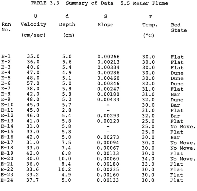
TABLE 3.3 Summary of Data 5.5 Meter Flume

U d S T

Run Velocity Depth Slope Temp. Bed

No. State (cm/sec) (cm) (*C) E-1 35.0 5.0 0.00266 30.0 Flat E-2 36.0 5.6 0.00213 30.0 Flat E-3 40.6 5.4 0.00334 30.0 Flat E-4 47.0 4.9 0.00286 30.0 Dune E-5 48.0 5.1 0.00460 30.0 Dune E-6 57.0 5.0 0.00346 32.0 Dune E-7 38.0 5.8 0.00247 31.0 Flat E-8 42.0 5.8 0.00180 31.0 Bar E-9 48.0 5.2 0.00433 32.0 Dune E-10 45.0 5.7 - 30.0 Bar E-11 45.0 2.8 - 31.0 Flat E-12 46.0 5.4 0.00293 32.0 Bar E-13 41.0 5.8 0.00120 25.0 Flat E-14 31.0 5.8 - 25.0 No Move. E-15 33.0 5.8 25.0 Flat E-16 42.0 5.8 0.00273 30.0 Bar E-17 31.0 7.5 0.00094 30.0 No Move. E-18 33.0 7.4 0.00067 30.0 No Move. E-19 42.0 6.8 0.00113 30.0 Flat E-20 30.0 10.0 0.00060 34.0 No Move. E-21 36.0 8.4 0.00180 33.0 Flat E-22 33.6 10.2 0.00235 30.0 Flat E-23 33.2 4.9 0.00160 30.0 Flat E-24 37.7 5.0 0.00133 30.0 Flat

- _______________ 3 .- '---.----..-. '.3-

~---.---.---TABLE 3.4 _{Reproducibility of Experimental Runs}

Run No.

Q, Discharge

A.5

(m 3/sec) 0.0484

d, Depth (cm) _15.3

U, Mean Velocity (cm/sec)

S, Friction Slope

T, Temperature (*C)

f, Friction Factor

Sediment Discharge (gm/cm sec x10-3) 34.6 0.00061 30.0 0.055 3.51 A.6 0.0464 14.8 34.4 0.00059 31.0 0.052 1.40 C.1 0.0503 15.8 34.8 0.00037 28.0 0.032 2.97

Bar Bar Flat

C.2 0.0530 16.3 35.4 0.00039 29.0 0.033 2.99

55

depth, and temperature. For the experimental pair

A5-A6, the slope and bed friction factor are again in

good agreement, but the sediment discharge is at variance. These experiments produced a bar bed configuration.

This variance of sediment transport rate does not necessarily imply a lack of reproducibility between these experiments or a poor sediment-discharge measurement. Rathbun and Guy (1967) made many measurements of bedload discharge in experiments in which ripples developed. The measure-ments displayed up to one hundred percent variance for

long sampling times and large sample sizes. To obtain a stable average sediment-transport rate in experiments with bed-form development, a very long sampling time would be necessary, and this massive sample would intro-duce irregularities in sediment resupply to the upstream end of the flume. It is concluded that for experimentally feasible sampling times there will be an inherent fluc-tuation in sediment transport rate as shown in A5-A6. The reproducibility of these experiments is therefore judged to be good.

BED CONFIGURATIONS Terminology

Southard (1971) has introduced convenient terms to describe the various aspects of any kind of bed

be used in this study.

A bed form is an individual structural element such as a ripple or dune.

A bed configuration is an individual or specific geometrical representation of the sand bed, such as a flat bed, a ripple-covered bed, or a bed with a complex assemblage of different bed forms. The term bed configuration is used to describe the geo-metry of the entire bed, whereas the term bed form

is used to describe an individual geometrical element of a bed configuration.

A bed state is the average or totality of all

particular bed configurations that can be formed by a given set of average flow conditions. For example, during a given run the bed configuration is different for every different time, but the bed state remains the same (i.e., the ripple bed state).

A bed phase is the aggregate of all bed states that involve a particular kind of bed configuration or a particular characteristic assemblage of bed configura-tions. For example, a series of flume runs for

different depths, velocities, and grain sizes could all be characterized as involving the dune bed state.

The totality of such dune bed states would constitute the dune bed phase, and the range of mean flow con-ditions (mean velocity, mean depth, grain size) within

which the dune phase exists would constitute the dune-phase stability field.

This definition of bed phase closely approximates that independently proposed by Pratt (1971) to divide hydrau-lically defined regions of similar bed-form development.

Terminology for specific bed configurations was discussed and defined by a Task Force of the Committee

on Sedimentation of the American Society of Civil Engineers (1966). The purpose of these definitions was to provide an unambiguous term for every kind of alluvial bed con-figuration. However, no attempt was made to provide terminology to characterize hierarchical succession of bed configurations, since at that time there was no

con-sensus as to the hydraulic criteria that accurately define the occurrence of each bed configuration. In the literature the terms bed form and bed configuration have been used

interchangeably and have included the meanings of the

terms bed form, bed configuration and bed state as defined here.

The bed configurations described in this chapter include flat bed with no movement, flat bed with grain movement, ripples, and dunes. One additional bed con-figuration, bars, will be introduced, and the detailed basis of distinguishing this bed configuration will be presented in the following sections of this chapter. Costello and Southard (1971) observed the bar bed form

58

in 1.14 mm sand and compared it to the bancs (bars)

described by Chabert and Chauvin (1963) in 0.96 mm sand. Pratt (1971) reported identical bed configurations in 0.49 mm sand and has called them "intermediate flattened dunes." Bars have lengths and heights comparable to dunes but do not have the regularity of spacing that

dunes display; also bars are largely two-dimensional, with straight crests and very little scour downstream of

the slipface, whereas dunes are more three-dimensional, with scour pockets downstream of the slipface.

In the following sections of this chapter, distinctions between different bed configurations will be made by

observing the effects of each bed configuration on the flow and by observing the actions and geometries of the bed configurations with changes in flow conditions. If the bed configuration is undergoing a transition rather than simply varying its form, the mean flow characteristics

(such as energy slope or friction factor) and the sand bed geometries (spacing or height of bed forms) should show recognizable changes in trends, as should observa-tions of kinematics of bed forms.

Observations

This section describes the observed differences in kinematics of bed configurations with increasing mean

quali-59

tative and are designed to define the bed phases. More detailed observations will follow in a later section of this chapter.

At velocities too low to cause grain movement, a leveled sand bed remains unchanged. Closeup observations of the sand bed revealed that sand grains sitting exposed above the bed level, or sand grains entrained by turbulence at the inlet, roll a short way down the bed until they

fill a vacant hole on the bed surface. Sand grains well packed into the bed surface are not moved or reoriented. In the finer sands, series A,B, and C, ripples can

develop on a bed with no grain movement: if a small

surface irregularity (2-3 grain diameters high) is present on the sand bed or one is introduced onto the bed, a train of ripples is observed to grow very slowly downstream

from the disturbance (Fig. 3.1). The ripple train pro-pagates downstream and later the upstream part of the ripple train spreads across the width of the flume.

At higher velocities, grains can be set in motion on the flat bed. Exposed grains, located above the average bed level, are the first to be move. More deeply imbedded grains are initially flipped over to produce an imbricated bed. Motion occurs in bursts which erode patches of motionless grains and roll them downstream until the grains find a protected shelter or vacant hole in the bed surface or until they reach

60

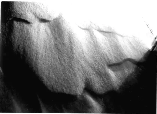
Fig. 3.1. Development of a ripple train from a line disturbance on a flat bed with no grain motion (Run C-7, D = 0.66 mm , flow from

Fig. 3.Z. Newly formed ripples in the flat bed(metastable ripple) phase (Run B-2, D =0.60 mm , flow from top to bottom). g