HAL Id: hal-01416760
https://hal.archives-ouvertes.fr/hal-01416760
Submitted on 15 Dec 2016
HAL is a multi-disciplinary open access
archive for the deposit and dissemination of
sci-entific research documents, whether they are
pub-lished or not. The documents may come from
teaching and research institutions in France or
abroad, or from public or private research centers.
L’archive ouverte pluridisciplinaire HAL, est
destinée au dépôt et à la diffusion de documents
scientifiques de niveau recherche, publiés ou non,
émanant des établissements d’enseignement et de
recherche français ou étrangers, des laboratoires
publics ou privés.
from Paris, Sao Paulo and Mumbai
Gaele Lesteven
To cite this version:
Gaele Lesteven. Behavioral Responses to Traffic Congestion - Findings from Paris, Sao Paulo and
Mumbai. TRA 2014, 2014, Paris, France. pp.121 - 138, �10.1002/9781119307822.ch9�. �hal-01416760�
Behavioral responses to traffic congestion.
Findings from Paris, São Paulo and Mumbai
Gaele Lesteven
**CRIA / UMR Géographie-Cités, Université Paris 1 Panthéon-Sorbonne, Paris, France updated version – Sept. 2015
Abstract
This paper focuses on the impacts of traffic congestion in the daily life of metropolitan motorized households. It is based on a doctoral dissertation defended in 2012 which studied three mega cities: Paris in France, São Paulo in Brazil and Mumbai (ex-Bombay) in India. A stated-adaptation survey (simulation game) was conducted in 2009-2010 to identify behavioural responses to traffic congestion and to estimate the threshold of household tolerance to congestion in the three regions. A universal set of fifteen responses was available to households in the three regions. Respondents first selected marginal adjustments then behavioural alterations. They managed to preserve their activity pattern thanks to a few marginal adjustments until they reached a threshold and started to alter their behaviour. The threshold was almost the same from one region to another. It fluctuated around 30 additional minutes of travel time. This result was consistent with the Zahavi’s conjecture of travel time budget stability.
Keywords: Traffic congestion; behaviour; mega city; stated-adaptation survey.
Résumé
Cet article analyse le rôle de la congestion automobile dans la vie quotidienne des ménages motorisés des grandes métropoles. Il est tirée d’une thèse soutenue en 2012 et consacrée à l’étude de trois grandes métropoles : Paris, São Paulo et Mumbai (ex-Bombay). Une enquête interactive de réponses déclarées (jeu de simulation) a été menée en 2009-2010 afin d’identifier les stratégies d’adaptation des ménages et d’estimer leur seuil de tolérance à la congestion. Les ménages disposent d’une liste de quinze stratégies différentes. Ils optent d’abord pour des stratégies d’ajustement marginal puis pour des stratégies d’altération. Ils réussissent à préserver leur programme d’activités, grâce à des ajustements marginaux, jusqu’à atteindre un seuil et commencer à modifier leur comportement. Le seuil est quasi-identique d’une métropole à l’autre. Il oscillerait autour de 30 minutes en plus de temps de parcours. Ce résultat confirme l’hypothèse d’une constance des budgets temps énoncés par Zahavi.
Mots-clé: automobile ; congestion ; comportement ; métropole ; enquête interactive de réponses déclarées.
1. Introduction
1.1. Traffic congestion
In mega cities, dealing with traffic congestion is a daily effort for many inhabitants (Downs, 2004). Traffic congestion happens because road supply cannot satisfy travel demand. Congestion mainly extends travel times and/or increases their variability. We wonder how households maintain their travel time budget and preserve their lifestyle in case of intense congestion. We suppose that households have to alter their travel patterns and even their activity patterns to maintain their travel time budget and preserve their lifestyle. The first aim of this paper is to draw up an exhaustive set of responses to traffic congestion. Do the responses differ from one mega city to another? Which responses are the most often selected? And for which reasons? The second aim is to estimate the threshold of tolerance to traffic congestion. We test the hypothesis that the higher is the stress due to congestion, the more households have to modify their activity patterns to maintain their lifestyle.
The remainder of this paper is organized as follows. Section 1.2 describes the context of the three studied mega cities. Section 2 explains the method and details the sample. Section 3 shows the results. Section 4 presents a final discussion.
1.2. The context of the three studied mega cities
We selected three constrated mega cities presenting three stages of motorization and belonging to three different cultural areas: the Paris metropolitan region (PMR) in France, the São Paulo metropolitan region (SPMR) in Brazil and the Mumbai metropolitan region (MMR) in India. First, we present the three metropolitan regions, then we focus on motorization, daily mobility and traffic congestion in these regions. The data presented in this section, otherwise noted, were obtained from three household travel surveys: the 2010 Global Transport Survey (DRIEA & STIF, 2012) for the PMR, the 2007 Origin-Destination Survey (METRÔ, 2007) for the SPMR and the 2008 Comprehensive Transport Study for Mumbai Metropolitan Region (MMRDA & LEA, 2008).
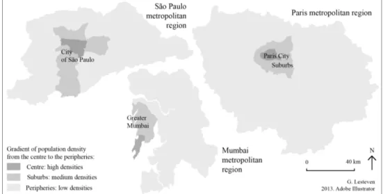
Figure 1 presents the three regions. Paris is the capital of France. The PMR (or Ile-de-France) covers an area of 12,000 km2 where 11.8 million people live. Population (57%) and employment (67%) are mainly concentrated in
Paris city and its suburbs. São Paulo is the capital of the State of São Paulo and the economic centre of Brazil. It is located in the south-east part of Brazil. The SPMR has a population of 20.1 million inhabitants within an area of 8,000 km2. 60% of the metropolitan region population lives and/or works in the city of São Paulo. Located on
the west coast of India, Mumbai is the capital of the State of Maharashtra and the economic capital of India. The area of the MMR is divided into a peninsula (which forms the municipality of Greater Mumbai) and the continent. It is smaller (4,350 km2) than the PMR and the SPMR. 60% of 20.7 million residents of the MMR live
in the peninsula. In the centre of the MMR, located at the end of the peninsula, the population density is very high (43,000 inhabitants/km2). It is more than twice the density of Paris city. Densities progressively decrease in
the north of the peninsula and in the continent. At the same time, jobs have been dispersed in the metropolitan region.
There are 430 cars for 1,000 inhabitants in the PMR. In Paris city, only 45% of the households own a car against 71% for the whole PMR. In the SPMR, motorization is lower: there are 180 cars per 1,000 inhabitants. 49% of the households of the SPMR own a car. Households who live in the centre of the SPMR are wealthier and more motorized (59%). Motorization in the MMR remains modest, with 33 cars per 1,000 inhabitants. Only 5.4% of the households in the MMR are motorized. The motorization rate is still higher in the centre where many wealthy households live.
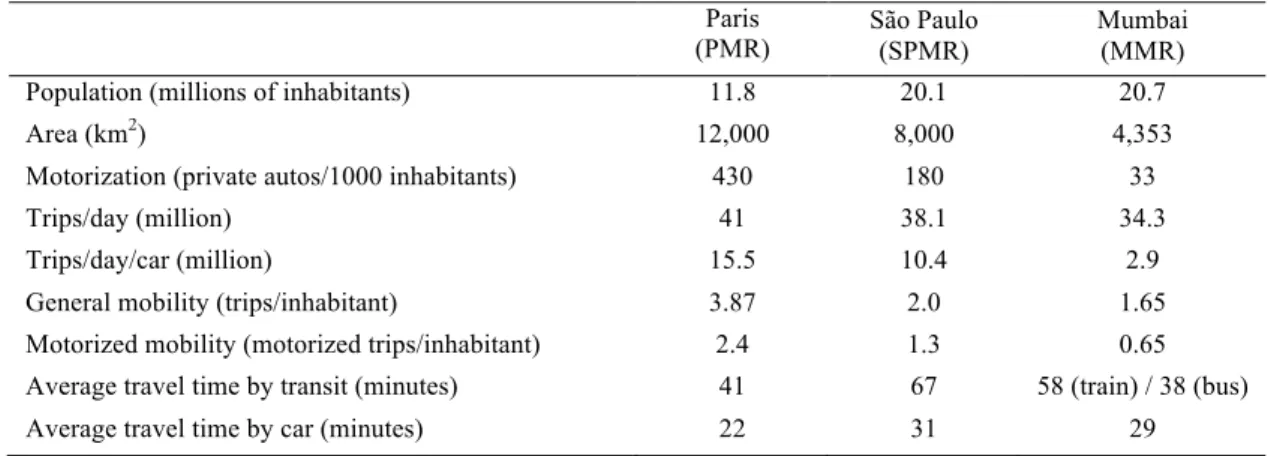
Table 1. General data
Paris
(PMR) São Paulo (SPMR)
Mumbai (MMR)
Population (millions of inhabitants) 11.8 20.1 20.7
Area (km2) 12,000 8,000 4,353
Motorization (private autos/1000 inhabitants) Trips/day (million)
Trips/day/car (million)
General mobility (trips/inhabitant)
Motorized mobility (motorized trips/inhabitant)
430 41 15.5 3.87 2.4 180 38.1 10.4 2.0 1.3 33 34.3 2.9 1.65 0.65 Average travel time by transit (minutes)
Average travel time by car (minutes)
41 22 67 31 58 (train) / 38 (bus) 29
In the PMR, the modal share of walking (39%) slighty exceeds the modal share of private cars (38%). The modal share of public transport is below (20% divided into 43% for the bus and 57% for the train plus the metro). In the SPMR, the ratio of walk trips is lower (34%) than in the PMR. It also the case for the modal share of private cars (30%). Bus trip share remains significant (29%), while the participation of rail and subway trips is low (8%). As in the PMR, walking trips are dominant in the MMR (61%). Train is the second more popular transport mode (20%), followed by bus (9%). Taxis and three-wheelers (auto rickshaws) represent 4% of trips. It is more than cars (3%) or motorized two-wheelers (3%).
Work remains the main purpose of travel in the PMR (29%). But its share is less important than in the SPMR (44% of trips are work trips) and in the MMR (46%). In the PMR, work-purpose travellers mainly use the car (44%), followed by public transport (40%). In the SPMR, they equally use the bus (31%) and the car (30%), while in the MMR, they mainly go by foot (40%) or by train (37%). Only few of them go to work by car (2%). Mobility in the PMR (3.87 trips per inhabitant per day) is greater than in the SPMR (1.97) and in the MMR (1.65). An PMR inhabitant spends 92 minutes travelling per day, instead of 83 minutes in 2001. In the SPMR, the travel time budget is 77 minutes per day. It is 15 minutes more than a decade before. A wealthy inhabitant spends 95 minutes travelling per day, while a poor inhabitant spends 48 minutes. 24% of wealthy people don’t travel against 46% of poor people and 55% of very poor people. The situation is similar in the MMR and the reasons are the same: lack of money and lack of jobs. Still 40% of wealthy MMR people don’t travel, which is a lot more than in the PMR and the SPMR.
Traffic congestion is characterized by low average travel speeds during peak periods. Daily average speed in Paris city has dropped from 20.9 km/h to 15.7 km/h in 20 years (Mairie de Paris, 2011). At the same time, traffic congestion on the PMR expressways remains moderately constant, even with the motorization growth in the suburbs, thanks mainly to traffic management. Nevertheless, average traffic speed during the day (7 am – 9 pm) has seen a little decrease. In the SPMR, the average traffic speed has decreased, especially during the evening peak hours: from 24.9 km/h in 1980 to 14.8 km/h in 2008 (CET, 2010). In the MMR, the minimum average speed had also decreased: from 18 km/h in 1962 to 8 km/h in 2008 in the centre and from 30 to 5 km/h in the suburbs (MMRDA & LEA, 2008).
In the PMR, traffic congestion mostly occurs in the suburbs and in the peripheries where most of motorized households live. Real estate prices in Paris city force both people and jobs to move from the city to the suburbs. The public transport system is efficient within Paris city and for linking the suburbs to the city. But it is less
efficient when travelling within the suburbs, for which the private car is preferred. Very different is the situation in the SPMR. There, the growth of private cars is concentrated in the centre, where traffic congestion is worse. The higher income groups that intensively use private cars invest much more time, space and money to travel around and so contribute to traffic congestion. In the peripheries, where poor and middle-income people live, mobility is seriously affected. In the MMR, the situation is similar: traffic congestion is the highest in the peninsula, while the road network has not changed much in 4 decades. Encroachments, mixed traffic and lack of traffic discipline also play a role.
2. Methodology
An earlier paper (Lesteven & Alves, 2011) presented the methodology more in depth and started to analyse the results of the survey conducted in Paris and in São Paulo.
2.1. Presentation of the method
In order to understand how metropolitan motorized households cope with daily congestion, we referred to simulation methods. Using simulation game offers an opportunity to put the respondents in situation and to observe all the possible behavioural responses without any a priori (Faivre d’Arcier, 2008). Jones (1980) was the first to explore the possibilities of gaming-simulation with HATS (Household Activity and Travel Simulator). Called stated-adaptation survey (or interactive stated response survey), this type of survey focuses the observation not only on the stated choices of the respondents, but also on their choice process (Le Vine et al, 2014; Habib et al, 2013).
The stated-adaptation survey we implemented was based on increasing travel times. It allowed us to comprehend behavioural responses to traffic congestion. The survey had two stages: 1) The respondent filled up a trip diary listing all trips, no matter what purpose or mode of transport was used, for several consecutive days. 2) During an in-depth face-to-face interview, the respondent reacted to hypothetical situations based on selected trips from the trip diary. The aim of the method was not to reach behavioural representativeness but to explore and understand the choice process. For this reason, the sample (15 to 20 households) for each case study was small (Faivre d’Arcier, 2008), but it had to be as diversified as possible. All the interviews were “tape” recorded. 2.2. The sample
The survey took place in the three case studies over a year: the SPMR in September - October 2009, the MMR in March - April 2010 and the PMR in January - February and May - June 2010 (Lesteven, 2012). We tried to avoid adverse weather conditions (snow or monsoon) and school holidays as much as possible. The selected households had to own at least one car and use it several times a week.
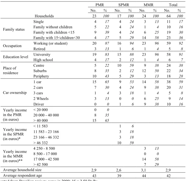
A sample of 64 motorized households (91 respondents) participed in the survey. Among them, 23 households (16 men and 15 women) lived in the PMR, 17 households (12 men and 11 women) in the SPMR, and 22 households (22 men and 15 women) in the MMR. Respondents were recruited by indirect relationships. At the end of the interview, they received a gift. In order to have a diverse sample, respondents first filled in a recruitment form. Too similar households were rejected. The sample was well diversified in terms of family status and places of residence. It came with no surprise that it was hard to interview low-income motorized households.The socio-economic characteristics of the sample are detailed in Table 2.
Table 2. Sample characteristics
PMR SPMR MMR Total
No. % No. % No. % No. %
Households 23 100 17 100 24 100 64 100
Family status
Single 4 17 4 24 3 13 11 17
Family without children 5 22 4 24 1 4 10 16
Family with children <15 9 39 4 24 6 25 19 30
Family with 15<children<30 4 17 5 29 14 58 23 36
Occupation Working (or student) 20 87 16 94 23 96 59 92
Retired 3 13 1 6 1 4 5 8
Education level University 19 83 15 88 23 96 58 91
High school 4 17 2 12 1 4 6 7 Place of residence Centre 5 22 10 59 9 38 24 38 Suburbs 8 35 2 12 12 50 22 34 Periphery 10 43 5 29 3 13 18 28 Car ownership 1 car 15 65 9 53 14 58 38 59 2 cars 7 30 4 24 9 38 20 31 3 cars 1 4 3 18 1 4 5 8 2 Wheels 3 13 0 0 6 25 9 14 Driver 0 0 1 6 9 38 10 16 Yearly income in the PMR (in euros) < 20 000 0 0 20 000 - 40 000 8 35 > 40 000 15 65 Yearly income in the SPMR (in euros)* < 11 583 1 6 11 583 - 23 166 3 18 23 166 - 46 332 3 18 > 46 332 10 59 Yearly income in the MMR (in euros)** 4 250 - 8 500 3 13 8 500 - 17 000 0 0 17 000 - 42 500 14 58 > 42 500 7 29
Average household size 2,9 2,6 3,1 2,9
Average respondent age 43 39 44 42
*converted from Brazilian reais to euros in 2009: 1€ = 2,59 Br Rs **converted from Indian roupies to euros in 2010: 1€ = 58,8 Indian Rs
2.3. Implementation of the survey
All the adult members of the household had to fill a trip diary during a whole week in the PMR and three consecutive days in the SPMR and the MMR. The aim was to identify travel and activity decisions which had been taken within the household during the trip diary filling process. Few days after completing the trip diary, the regular car drivers of the household were interviewed.
First, the interviewer reminded the respondents about the contents of the trip diary and asked the respondents to select three representative types of trips. Most of the time, the selected compulsory trip was a commute trip or a drop children off to school trip. The selected non-compulsory trip occurred mostly for shopping or leisure. The selected travel time budget (TTB) was the sum of the trips made during the most representative day of the trip diary. The revealed travel time (RTT) referred to the amount of time the respondents quoted for these trips in their trip diary.
Then, two scenarios were tested. Scenario 1 considered non-recurrent congestion, presenting variable and unpredictable travel times. Scenario 2 concerned recurrent congestion, presenting longer travel times. For both scenarios, the compulsory and the non-compulsory trips were taken into account. The TTB was considered only for scenario 2. Each scenario was built in three levels corresponding to three levels of change in travel conditions
(+50%, +100% and +200%). Each level was presented as a pre-filled playing card. The playing cards were progressively shown to the respondent (levels 1, 2, 3 of scenario 1; then levels 1, 2,3 of scenario 2). Respondents were expected to state how the change in travel conditions described in each card would affect their travel and activity patterns. Most of the time, other members of the household were present during the interview to check the validity of the respondent’s stated responses. Table 3 presents the two scenarios.
Table 3. The two scenarios
Scenario 1
Non-recurrent congestion
Scenario 2
Recurrent congestion
Under test Variable & unpredictable travel times Longer travel times
Data selection A regular & compulsory trip (e.g. a commute trip)
A regular & non compulsory trip
A regular & compulsory trip A regular & non compulsory trip Whole day trips (travel time budget) 3 levels of changes
in travel conditions
1/Between the revealed travel time (RTT) & +50% RTT 2/Between the RTT & 2x RTT
3/Between the RTT & 3x RTT
1/+ 50% of revealed travel time 2/ RTT x 2
3/ RTT x 3
3. Results
3.1. A universal list of responses to traffic congestion
The first aim of the survey was to establish an exhaustive list of behavioural responses to traffic congestion. According to Mokhtarian et al. (1997), motorized households deal with a universal set of behavioural responses to traffic congestion, regardless of their family status, their level of income or their place of residence. This does not mean that a household takes all strategies listed but it selects some of them, according to its constraints and resources. Mokhtarian et al. (1997) proposed a universal set of 16 possible responses based on a survey conducted in San Diego, California, in 1992. Bovy and Salomon (2002) summed up the universal set into 11 strategies: 1. Accept travel costs (do-nothing situation); 2. Reduce travel costs (a more comfortable vehicle); 3. Adapt departure time; 4. Change route; 5. Buy time (e.g. use toll roads); 6. Temporal changes (flexitime, compressed work week); 7. Change mode; 8. Telecommute; 9. Relocation of place of workplace or home; 10. Start a home-based business; 11. Quit work. We wonder if this universal set is still accurate today in these different metropolitan regions.
In the survey we conducted in the PMR, the SPMR and the MMR, the 91 respondents answered up to 15 playing cards (6 playing cards for the compulsory trip related to scenarios 1 and 2; 6 cards for the non-compulsory trip; 3 cards for the TTB related to the scenario 2). Sometimes, it was not relevant for the respondent to answer to all the cards (such as the respondent who didn’t use his/her car to go to work). Respondents were free to answer what they wanted. Most of the time, they stated one response per card, i.e. per level of scenario. Some of the respondents gave a second response (14% of responses), even a third (2%). 1.142 responses were counted and listed. At the end, 15 different behavioural responses were found. Regarding their impacts on household travel and activity patterns, the 15 behavioural responses can be organized in five groups. Group 1 consists of marginal adjustments (“maintain behaviour”, “leave earlier”, “change route”). They could slightly affect household travel patterns. The four remaining groups are composed of behavioural alterations. Group 2 is modal alterations (“other mode”, “carpool”, “have a driver”), group 3 temporal alterations (“reschedule”, “decrease frequency”, “change shift”) and group 4 spatial alterations (“change destination”, “chain trips”, “work from home”). Modal, spatial and temporal alterations affect household travel patterns and even activity patterns. Radical alterations, which name the group 5 (“quit”, “quit job”, “move”), are ruptures in the activity pattern.
All the 15 responses occurred in the three regions, except for the response “driver” which was specific to the MMR. In Mumbai, many people have a driver. They drive about 70% of the private cars on weekdays (Datar, 2010). In the sample, which was not representative, 9 of the 24 MMR households employed a driver. They considered the private car as a “private taxi” (MMRDA & LEA, 2008). Having a driver is probably the most efficient response to traffic congestion. The activity pattern remains well and comfortably preserved. Nevertheless, having a driver in Mumbai is a privilege of high-income households, even more than owning a
private car. We assume that the number of drivers will progressively reduce with the democratisation of private cars, as it is already the case in Delhi.
Table 4 presents the number of times each response was stated per type of trip (compulsory, non-compulsory, TTB), without specifying the scenario. The assumption of a universal set is confirmed.
Table 4. The 15 behavioural responses and the number of times they occurred
Responses
Paris (PMR) São Paulo (SPMR) Mumbai (MMR)
Groups C NC TTB C NC TTB C NC TTB
Marginal 1. Maintain behaviour 60 55 23 23 39 5 42 52 16
Adjustments 2. Change departure time 44 0 2 49 17 8 55 8 6
3. Change route 14 7 0 18 8 3 7 5 1
Modal 4. Other mode 23 16 8 18 12 8 24 13 24
Alterations 5. Carpool 0 0 2 2 0 1 4 1 1
6. Have a driver 0 0 0 0 0 2 0 1 8
Temporal 7. Decrease frequency 2 9 1 1 17 0 1 11 4
Alterations 8. Reschedule 3 14 1 7 15 4 14 11 4
9. Change shift 5 1 1 6 0 1 1 4 2
Spatial 10. Chain trips 1 2 3 0 1 5 1 1 1
Alterations 11. Change destination 0 15 2 5 18 4 5 17 3
12. Work from home 3 0 0 5 0 3 9 0 1
Radical 13. Quit 6 8 2 6 13 15 9 19 6
Alterations 14. Quit job 8 0 5 1 0 2 10 0 7
15. Move 5 0 7 15 0 7 4 0 7
Number of times 174 127 57 156 140 68 186 143 91
C: Compulsory trip (scenarios 1 & 2); NC: Non-compulsory trip (scenarios 1 & 2); TTB: Travel Time Budget (scenario 2).
Interestingly, the universal list Mokhtarian et al. made up and Bovy & Salomon completed has not changed a lot in the last twenty years. The differences come from the technological progress and the comfort it offers: it is today common to own a car radio and a cell phone.
3.2. Different frequencies
We would like to know which responses among the 15 listed were stated the most often and for which reasons. We suppose that households try to preserve their activity pattern as much as they can, because it is the result of negotiations within the household (Vovsha et al., 2004). This is why we assume that the responses that are the most common are marginal adjustments, followed by alterations. Table 5 details the frequency of the responses.
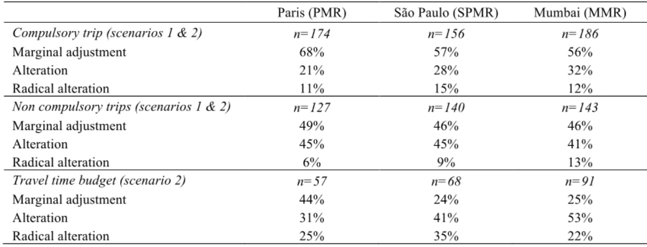
Table 5. The frequency of the responses per trip for each region
Paris (PMR) São Paulo (SPMR) Mumbai (MMR)
Compulsory trip (scenarios 1 & 2) n=174 n=156 n=186
Marginal adjustment 68% 57% 56%
Alteration 21% 28% 32%
Radical alteration 11% 15% 12%
Non compulsory trips (scenarios 1 & 2) n=127 n=140 n=143
Marginal adjustment 49% 46% 46%
Alteration 45% 45% 41%
Radical alteration 6% 9% 13%
Travel time budget (scenario 2) n=57 n=68 n=91
Marginal adjustment 44% 24% 25%
Alteration 31% 41% 53%
The hierarchy in which the most common responses are those that affect the least the activity pattern was respected for compulsory trips. The hierarchy began to fail for non-compulsory trips. Respondents tended to alter their behaviour a little more. They mostly changed their destination (spatial alternation) and reschedule their trip (temporal alteration). Contrary to compulsory trips, destination and time were not forced. They preferred to keep their car and cancelled the trip if travel times were too long (levels 2 and 3). In the case of travel time budget, the hierarchy was confirmed in the PMR but not in the SPMR and in the MMR. The respondents from São Paulo and Mumbai regions altered their behaviour more than the respondents from Paris region.
A second analysis focused on the length of the trips and if it affected the hierarchy. First, we looked at short trips, for which the revealed travel time was equal to or shorter than 30 minutes, then at long trips (a revealed travel time of more than 30 minutes). The hierarchy was confirmed, except for long compulsory trips. Marginal adjustments were more common for short trips and alterations for long trips. In fact, the length and the compulsory nature of the trips were two factors determining the behaviour of respondents.
3.3. The threshold of household tolerance to congestion
The second aim of the survey was to estimate the threshold of household tolerance to traffic congestion. We wanted to test the hypothesis that the higher is the stress due to traffic congestion, the more households have to modify their travel and activity patterns to maintain their lifestyle.
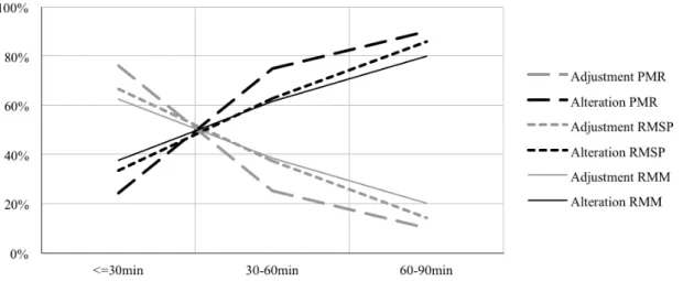
We created a new variable called variable of delay. The delay was the time added to the revealed travel time at each level of scenario 2. For example, the delay would be 15 minutes if a revealed travel time of 30 minutes were increased by 50% (level 1). It would be 30 minutes if the revealed travel time were doubled (level 2) and 60 minutes if it were trebled (level 3). We wondered what the delay was when the respondents started to alter their behaviour. Figure 2 shows the results for compulsory trips in the second scenario. The threshold matched with the intersection of the curve of marginal adjustments and the curve of alterations. Delays were grouped in three periods of time: less than 30 minutes, 30-60 minutes and 60-90 minutes. The threshold of household tolerance to congestion was almost the same from one region to another. It fluctuated around 30 minutes in addition to the revealed travel time. When travel times exceeded these 30 minutes, respondents started to alter their behaviour. Up to an additional half-hour travel time, people managed to preserve their activity pattern thanks to a few marginal adjustments (such as changing the departure time, changing the itinerary route, using the phone, etc).
Fig. 2. Behavioural thresholds according to the delay in scenario 2 for compulsory trips
This result cannot be applied generally because of the non-representative sample. But it appears to be consistent with the surveys of Stern (2002) and Weis et al. (2010). Stern conducted a revealed preference survey of 160 car drivers in the Tel Aviv region. He estimated a threshold for compulsory trips that varied between 30 minutes and one hour. Weis et al. conducted a stated-adaptation survey of 84 households living in the Zurich region about their behavioural responses to longer travel times, not only regarding car trips but all the trips they did. Their scenario was close to our scenario 2. There were 4 levels (+50%, +100%, +200%, -50%). Their respondents
preserved their activity pattern as much as they could. First, they reduced time at home before cancelling non-compulsory trips, then non-compulsory trips. From 90 minutes of additional travel time, they adopted radical alterations. In our survey, radical alterations started to be more common in the period of “60-90 minutes”.
4. Conclusions
According to the results of the survey, most of the metropolitan motorized households manage to preserve their lifestyle when facing growing congestion. They continue to use their car, even when the degrees of congestion increase. It confirms the fact that the effects of congestion on the automobile-based system are minor compared to the effects of car dependence (Dupuy, 2011). What is even more interesting is that the households are aware of this fact. In order to preserve their lifestyle, households first select marginal adjustments that affect their activity pattern the least. Then they use alterations and, only at the end, radical alterations. These results are based on a simulation game. We suppose that in real life, repondents are even more resistant to traffic congestion. In the game, respondents knew that the scenarios were composed of successive increases of travel time. This increasing bid may have prompted them to diversify their responses.
Respondents from the Paris region appeared to be less flexible than respondents from the SPMR and the MMR. They seemed to keep marginal adjustments as long as they could. Then they directly switched to radical alterations. There are several possible explanations for their lower degree of flexibility. Since the last 30 years, median and average travel times to work in the PMR have remained stable at around 30 minutes. At the same time, the PMR has sprawled and commute distances have doubled. The existence of a threshold of tolerance in terms of travel times for commute trips seems to be constituent of a metropolitan way of life. It could explain this stability of travel times to work (Massot, 2010). Moreover, some commuters may be unwilling to sacrifice the comfort and flexibility of the private car just to save a minor amount of time (Kent, 2014).
Most of the respondents in the survey stated that even in bad traffic conditions, they would manage to preserve their activity terms thanks to short-term strategies (marginal adjustments) or medium-term strategies (modal, spatial and temporal strategies) until they reach the threshold of tolerance of about 30 addditional minutes of travel time. It is interesting to notice that the threshold of tolerance to traffic congestion was more or less the same in the three regions. This is consistent with the Zahavi’s conjecture of travel time budget stability (Zahavi, 1974). People maximise their travel distances according their travel time budget (TTB) and their travel cost budget. Motorization increases the speed and reduces travel times (it takes less time to drive the same distance with higher speed). With the access to motorization, the TTB decreases. Then it stops to a level where the average TTB doesn’t reduce itself anymore and becomes stable (Crozet & Joly, 2004). The daily TTB is about one hour. Its tends to increase with the size of the city (about one hour 30 minutes in mega cities). The fact that respondents eventually reached a threshold supports the Zahavi’s conjecture.
To conclude, we noticed that from one region to another, the set of behavioural responses was similar. But household behaviours were not identical. The differences in behaviour could be explained by the place of residence of the motorized households in the metropolitan regions and the location of traffic congestion. As the origin-destination analysis pointed out in Section 1, motorized households in the SPMR and the MMR are most of the time wealthy households who mainly live in the centre of the metropolitan regions. In the PMR, motorized households mostly live in the periphery areas of the metropolitan region and tend to belong to middle or low-income classes. Traffic congestion mainly occurs in the centre of the SPRM and the MMR. Very different is the picture of the Paris region. There, the traffic congestion has sprawled out of the city to the main roads of the suburbs and the peripheries. Because of the lack of efficient public transport from periphery to periphery, the PMR households continue to use their cars. Even when travel times increases a lot, the private car remains competitive compared to public transport. This assumption should be tested in a further research. Moreover, it would be interesting to estimate the probability of switching to public transport according to higher private car travel times in these mega cities. For example, a research about Berlin showed that the probability to use public transport was more than 50% when the travel time by public transport was inferior to 1.5 the travel time by car (Reinhold, 2008).
Acknowledgements
This paper is based on a recent doctoral research funded by Renault and defended at the University of Paris 1 Pantheon-Sorbonne in 2012, under the supervision of Prof. Gabriel Dupuy. The survey in the SPMR was conducted with the help of Prof. O. Strambi and B. Alves from the Polytechnic School of the University of São Paulo. The survey in the MMR was conducted with the help of A. Datar and S. Kelkar from Mumbai Environmental Social Network.
References
Bovy, P., & Salomon, I. (2002). Congestion in Europe: Measurements, patterns and policies. In E. Stern, I. Salomon, & P. Bovy (Eds.), Travel behaviour: Spatial Patterns, Congestion and Modelling (pp. 143-179). Cheltenham: Edward Elgar Publishing.
CET (2010). Relatório de Atividades Operacionais. São Paulo: Companhia de Engenharia de Tráfego.
Downs, A. (2004). Still Struck in traffic. Coping with peak-hour traffic congestion. Washington, D.C.: The Brookings Institution.
Crozet, Y., & Joly, I. (2004). Budgets temps de transport : les sociétés tertiaires confrontées à la gestion paradoxale du “bien le plus rare”. Les Cahiers Scientifiques du Transport, 45, 27-48.
Datar, A. (2010). Why Mumbai faces Traffic Jams more frequently in more areas? And car centric policies are making it worse. Working Paper. Mumbai: Mumbai Environmental Social Network.
DRIEA & STIF (2001). Enquête Globale Transport. Paris: Direction régionale et interdépartementale de l’équipement et de l’aménagement d’Ile-de-France.
Dupuy, G. (2011). Towards Sustainable Transport: The Challenge of Car Dependence. Montrouge: John Libbey.
Faivre d’Arcier, B. (2008). Explorer les changements de comportements et d’attitudes face à l’automobilité. In F. Clochard, A. Rocci, & S. Vincent (Eds.). Automobilités et altermobilités. Quels changements ? (pp. 133-145). Paris: L’Harmattan.
Habib, K. N., Sasic, A., Weis, C., & Axhausen K. (2013). Investigating the nonlinear relationship between transportation system performance and daily activity–travel scheduling behaviour. Transportation Research Part A, 49, 342–357.
Jones, P. (1980). Experience with Household Activity-Travel Simulator (HATS), Consumer Perspectives. Transportation Research Board, 765, 6-12.
Kent, J. (2014). Driving to save time or saving time to drive? The enduring appeal of the private car?. Transportation Research Part A, 65, 103-115.
Lesteven, G. (2012). Les stratégies d’adaptation à la congestion automobile dans les grandes métropoles : analyse à partir des cas de Paris, São Paulo et Mumbai, Thèse en géographie et aménagement dirigée par G. Dupuy, Paris, Université Paris 1 Panthéon-Sorbonne.
Lesteven, G., & Alves, B. (2011). Behavioral responses to traffic congestion. Findings from São Paulo and Paris. Transportes, 19-2, 42-48.
Le Vine, S., Adamou, O., & Polak, J. (2014). Predicting new forms of activity/mobility patterns enabled by shared-mobility services through a needs-based stated-response method: Case study of grocery shopping. Transport Policy, 32, 60-68.
Massot, M. - H. (Eds.) (2010). Mobilités et modes de vie métropolitains. Les intelligences du quotidien, Paris: L’Œil d’Or.
Mairie de Paris (2011). Paris transport and travel 2011 report. Paris: Mairie de Paris.
METRÔ (2007). Pesquisa Origem e Destino 2007 – Região Metropolitana de São Paulo. São Paulo: Metrô. MMRDA & LEA (2008). Comprehensive Transport Study for Mumbai Metropolitan Region. Mumbai: Mumbai Metropolitan Region Development Authority.
Mokhtarian, P. L., Raney, E., & Salomon, I. (1997). Behavioral response to congestion: Identifying patterns and socio-economic differences in adoption. Transport Policy, 4 (3), 147-160.
Reinhold, T., & Kearney, A. T. (2008). More passengers and reduced costs - the optimization of the Berlin public transport network. Journal of Public Transportation, 11 (3), 57–76.
Stern, E. (2002). Congestion in Europe: Measurements, patterns and policies. In E. Stern, I. Salomon, & P. Bovy (Eds.), Travel behaviour: Spatial Patterns, Congestion and Modelling (pp. 218-232). Cheltenham: Edward Elgar Publishing.
Vovsha, P., Bradley, M., & Bowman, J. (2004). Activity-based travel forecasting models in the United States: Progress since 1995 and Prospects for the Future. EIRASS Conference on Progress in Activity-Based Analysis, Maastricht.
Weis, C., Dobler, C. & Axhausen, K. (2010). Stated Adaptation Survey of Activity Scheduling Reactions to Changing Travel Conditions: Field Work and Preliminary Results. 12th WCTR Conference. Lisbon.
Zahavi, Y. (1974). Travel time budgets and mobility in urban areas. Washington DC: United States Department of Transportation.