HAL Id: tel-00976619
https://tel.archives-ouvertes.fr/tel-00976619
Submitted on 10 Apr 2014
HAL is a multi-disciplinary open access archive for the deposit and dissemination of sci-entific research documents, whether they are pub-lished or not. The documents may come from teaching and research institutions in France or abroad, or from public or private research centers.
L’archive ouverte pluridisciplinaire HAL, est destinée au dépôt et à la diffusion de documents scientifiques de niveau recherche, publiés ou non, émanant des établissements d’enseignement et de recherche français ou étrangers, des laboratoires publics ou privés.
oceanic models
Giovanni Abdelnur Ruggiero
To cite this version:
Giovanni Abdelnur Ruggiero. A comparative study of data assimilation methods for oceanic models. Earth Sciences. Université Nice Sophia Antipolis, 2014. English. �NNT : 2014NICE4011�. �tel-00976619�
Universit´e Nice Sophia-Antipolis - UFR Sciences
Ecole Doctorale Sciences Fondamentales et Appliqu´ees
T H `
E S E
pour obtenir le titre de
Docteur en Science
de l’Universit´e Nice Sophia-Antipolis
Sp´
ecialit´
e : Science de la Plan`
ete et de l’univers
pr´esent´ee et soutenue par
Giovanni RUGGIERO
Une ´
etude comparative de m´
ethodes d’assimilation
de donn´
ees pour des mod`
eles oc´
eaniques.
A comparative study of Data Assimilation methods
for oceanic models.
Th`ese dirig´ee par Jacques BLUM et Yann OURMI`ERES
soutenue le 13 Mars 2014
Jury
Mark Asch Rapporteur
Didier Auroux Examinateur Joaquim Ballabrera Poy Examinateur Jacques Blum Directeur de th`ese Pierre Brasseur Rapporteur Emmanuel Cosme Examinateur
Yann Ourmi`eres Co-directeur de th`ese Jacques Verron Examinateur
Remerciements
Tout d’abord j’aimerais remercier les deux Jacques qui ont rendu possible la r´ealisation de cette th`ese: Jacques Verron pour avoir cherch´e un financement pour que je puisse faire une th`ese sur l’assimilation de donn´ees en France et Jacques Blum pour m’avoir accept´e et m’avoir accueilli avec une telle gentil-lesse et attention qui ont fait disparaitre toutes les difficult´es culturelles que je pouvais exp´erimenter comme nouveau th´esard en France et surtout au LJAD.
Je remercie ´egalement Yann Ourmi`eres, mon co-directeur de th`ese, pour les r´eflexions et l’aide pour la r´edaction de la th`ese, et Emmanuel Cosme pour toute sa attention et les nombreuses discussions sur l’assimilation de donn´ees, vous avez ´et´e tr`es importants dans la d´emarche de cette th`ese.
Mes remerciements s’adressent aussi `a Mark Asch et Pierre Brasseur pour avoir accept´e aimable-ment de rapporter sur ma th`ese.
Je remercie aussi Didier Auroux, Joaquim Ballabrera Poy, Emmanuel Cosme et Jacques Verron pour m’avoir accord´e l’honneur de faire partie du jury de ma th`ese.
Je remercie egalement H´el`ene Politano et Severine Rigot pour leur disponibilit´e et leur assistance `a l’Ecole Doctorale.
Mes remerciements `a tout le personnel du LJAD, sp´ecialement `a Isabelle De Angelis et `a Jean Paul Pradere.
Un remerciements amical `a Jean-Marc Lacroix et `a Julien Maurin qui ont surtout assur´e les moyens informatiques n´ecessaires `a mes travaux.
Je remercie aussi Brice Eichwald pour m’avoir beaucoup aid´e avec la langue fran¸caise et toutes les d´emarches bureaucratiques. Lord Bienvenu, Nancy Abdallah et Camilo Garcia pour les bons moments pass´es ensembles.
Un remerciement tr`es special `a mon ami Sami Sassi qui fait partie de ma famille en France. Je remercie mes parents pour ˆetre toujours `a mon cot´e, grˆace `a eux j’en suis l`a !
Enfin, je remercie ma compagne Leticia qui partage sa vie avec moi depuis huit ans et sans laquelle je ne pourrais pas passer les moments de travail les plus durs. Espero poder abrir muitas cortinas contigo e com a nossa Dorinha.
Contents
1 Introduction 9
1.1 Introduction (French) . . . 9
1.2 Introduction . . . 16
2 Data Assimilation Methods 23 2.1 Introduction . . . 24
2.2 Preliminary Concepts . . . 24
2.3 Four Dimensional Variational Method - 4Dvar . . . 27
2.4 The Back and Forth Nudging . . . 30
2.4.1 Forward Nudging . . . 30
2.4.2 Backward Nudging . . . 33
2.4.3 Iterating the Forward and the Backward Nudging . . . 34
2.5 Bayesian Estimation . . . 37
2.5.1 Kalman Filter . . . 39
2.5.2 Kalman Smoothers . . . 47
2.5.3 Iterative Kalman Smoothers . . . 56
2.5.4 Probabilistic Four Dimensional Variational Method . . . 62
2.6 Numerical Implementation . . . 63 2.6.1 D-BFN . . . 63 2.6.2 Kalman Filter/Smoothers . . . 63 2.6.3 4Dvar . . . 64 2.7 Conclusions . . . 64 i
3 Ocean model 67
3.1 Introduction . . . 68
3.2 Primitive Equation Ocean Model . . . 68
3.3 The Model discretization . . . 70
3.3.1 Spatial discretization . . . 70 3.3.2 Temporal discretization . . . 71 3.4 Model parameterizations . . . 72 3.4.1 Horizontal physics . . . 73 3.4.2 Vertical physics . . . 73 3.5 Boundary conditions . . . 74 3.5.1 Lateral boundary . . . 74 3.5.2 Surface boundary . . . 74 3.5.3 Bottom boundary . . . 74
3.6 The backward integration . . . 75
3.6.1 Numerical aspects . . . 75
3.7 Model configuration . . . 77
4 Diffusive Back and Forth Nudging Experiments 79 4.1 Introduction . . . 80
4.2 Data Assimilation methods . . . 82
4.2.1 Diffusive Back and Forth Nudging - DBFN . . . 82
4.2.2 Four Dimensional Variational Method - 4DVar . . . 85
4.3 Data Assimilation Experiments . . . 86
4.4 Comments on the model physics . . . 88
4.5 The backward integration without Nudging: Practical aspects . . . 89
4.6 Data Assimilation Results . . . 95
4.6.1 Experiments with scalar nudging coefficients . . . 95
4.6.2 The Hybrid DBFN . . . 108
4.7 Conclusions and perspectives . . . 117
4.8 Appendix . . . 119
4.8.1 Ordinary Least Squares regression (OLS) . . . 119
CONTENTS iii
4.8.3 Numerical Results . . . 123
5 Diffusive Back and Forth Kalman Filter 129 5.1 Introduction . . . 130
5.2 Objectives . . . 132
5.3 Data Assimilation Experiments . . . 132
5.3.1 Filter and smoother initialization . . . 132
5.3.2 Covariance localization and inflation . . . 133
5.3.3 Observations Network . . . 134
5.4 Results . . . 135
5.4.1 Effect of the DA window and the covariance matrix rank . . . 135
5.4.2 Effect of iterations on the initial condition estimation and inno-vation statistics . . . 138
5.4.3 Effect of iterations on the covariance matrix structure . . . 144
5.4.4 Stability of the assimilation system . . . 148
5.4.5 The forecast performance . . . 151
5.5 Conclusions . . . 152 6 Conclusions 155 6.1 Conclusions (French) . . . 155 6.1.1 Principaux r´esultats . . . 155 6.1.2 Questions ouvertes . . . 156 6.1.3 Perspectives . . . 157 6.1.4 Remarques finales . . . 158 6.2 Conclusions . . . 159 6.2.1 Main findings . . . 159 6.2.2 Open questions . . . 160 6.2.3 Perspectives . . . 161 6.2.4 Concluding Remarks . . . 161
List of Figures
1.1 Skill of the 36 hour (1955–2004) and 72 hour (1977–2004) 500 hPa fore-casts produced at NCEP. Forecast skill is expressed as a percentage of an essentially perfect forecast score. Extracted from Lynch (2008). . . 17 1.2 Typical Mediterranean Sea observational network for a 10day time window. 18 1.3 Surface velocity for experiments employing the same forcing fields but on
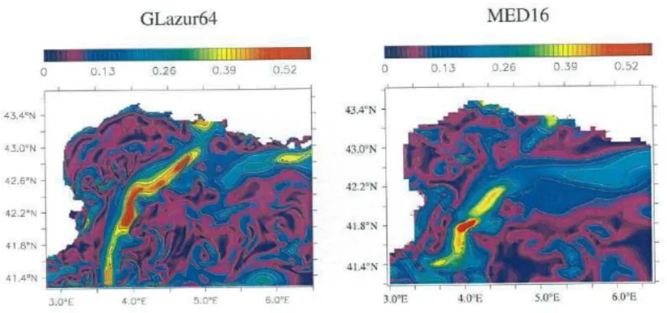
the right using spatial resolution of 1.7km (Glazur64) and on the left of 7km (MED16). Figures adapted from Duchez (2011). . . 19
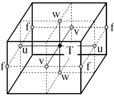
3.1 Arrangement of variables. T indicates scalar points where temperature, salinity, density, pressure and horizontal divergence are defined. (u, v, w) indicates vector points, and f indicates vorticity points where both rela-tive and planetary vorticity are defined. . . 72 3.2 Figures show the double gyre formation and evolution. Left panel: SSH
calculated after 1 day simulation. Right panel: SSH calculated after 70 years simulation. For the latter, it is observed a meandering jet and eddy structures. . . 78
4.1 Errors of the initial condition after one forward-backward model inte-gration perfectly initialized and without nudging. Red curves were ob-tained using the same diffusion coefficients used in the reference exper-iment (νhu,v = −8 × 10¹⁰m4/s and νt,s
h = −4 × 10¹¹m4/s) and magenta
curves were obtained using reduced diffusion (νhu,v = −8 × 10⁹m4/s and
νht,s = −8 × 10¹⁰m4/s). The abscissa represents the size of the time
window. . . 90
4.2 Vertical errors of the initial condition after one forward-backward model integration without nudging. Each color refers to an experiment per-formed using the diffusion coefficient indicated in the figure legend. The experiment represented by the dashed red curve used the same configu-ration as the experiment represented by the magenta curve but with a time step of 90s instead of 900s. Top panel: temperature errors; Bottom panel: zonal velocity errors. The time window is indicated in the title of each figure. . . 91 4.3 Sea level errors after one forward-backward model integration. The time
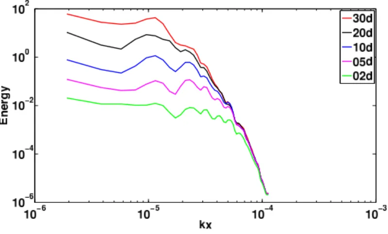
window is 10 days. . . 92 4.4 Mean power spectra energy calculated with the SSH error of one
forward-backward iteration. Each color represents a DA window: 2, 5, 10, 20 and 30 days. kx stands for longitudinal wave-number. . . 93 4.5 Kinetic energy mean power spectra calculated using the first layer
ve-locity fields. Black curves represent the “true“ initial condition power spectra; Red curves represent the power spectra calculated after one forward-backward iteration without the nudging term and employing the reference diffusion coefficient; Magenta curves represent the power spec-tra calculated after one forward-backward iteration without the nudging term and employing a reduced diffusion coefficient. Top left: 5 days as-similation window. Top right: 10 days asas-similation window. Bottom: 20 days assimilation window. In the bottom abscissa the ticklabels stand for longitudinal wave-number (rad/m) while in the top abscissa the tick-labels stand for the corresponding wavelengths in km units. . . 93 4.6 Relative errors of the zonal velocity (top) and the temperature (bottom)
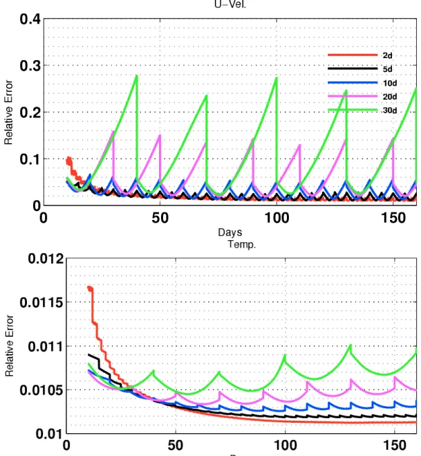
for the experiments listed in table 4.1 which assimilates SSH using the convergence criterion and the reference diffusion coefficient. . . 96 4.7 Relative errors of the zonal velocity (top) and the temperature (bottom)
for the experiments listed in table 4.1 which assimilates velocity using the convergence criterion and the reference diffusion coefficient. . . 97
LIST OF FIGURES vii
4.8 Relative errors of the zonal velocity (top) and the temperature (bottom) for the experiments listed in table 4.1 which assimilates SSH using the convergence criterion and the reduced diffusion coefficient. . . 100 4.9 Relative errors of the zonal velocity (top) and the temperature (bottom)
for the experiments listed in table 4.1 which assimilates velocity using the convergence criterion and the reduced diffusion coefficient. . . 101 4.10 Variation of the initial condition relative errors with respect to the
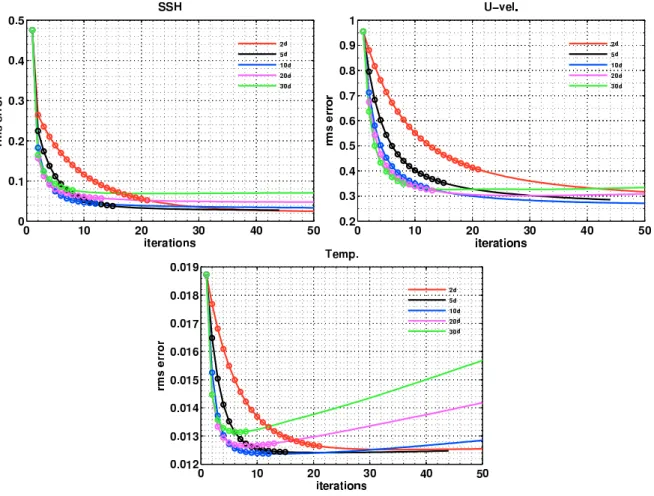
it-erations for the experiment assimilating daily gridded SSH fields. The circles represent the results obtained using the standard convergence cri-terion, ǫ = 0.005, and the continous lines obtained with a more restrictive criterion ǫ = 0.001. Top left: SSH error; Top right: zonal velocity error; Bottom: temperature error. . . 103 4.11 Relative errors of the zonal velocity (top) and the temperature (bottom)
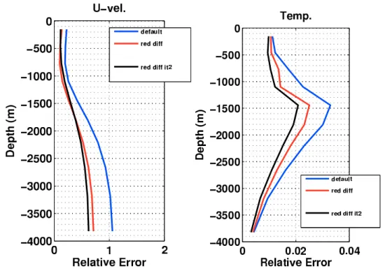
for the experiments listed in table 4.1 which assimilates SSH using only two iterations. All experiments have used reduced diffusion coefficients. 105 4.12 Vertical relative error of the zonal velocity (left) and the temperature
(right) for the experiments ssh 10d dd (default), ssh 10d rd (red diff) and ssh 10d rd 2it (red diff it2). The data refers to the identified initial conditions of the first assimilation cycle. . . 106 4.13 Vertical relative error of the zonal velocity (left) and the temperature
(right) for the experiments ssh 10d dd (default), ssh 10d rd (red diff) and ssh 10d rd 2it (red diff it2). The data refers to the identified initial conditions of the last assimilation cycle. . . 107 4.14 Relative errors of the zonal velocity (top) and the temperature (bottom)
for the experiments ssh 10d rd (red curve) and ssh 10d rd it2 (dashed red curve) and their equivalents but with K constructed using PLS regression (black curves). . . 109 4.15 . . . 110
4.15 (a and d) Root Mean Squared errors of zonal velocity for the experiments ssh 10d rd (red curve) and ssh 10d rd it2 (dashed red curve) and their equivalents but with K constructed using PLS regression (black curves). (b and e) First EOF mode and (c and f) second EOF mode calculated with the zonal velocity error. Top/bottom panel are results of the 1o/130o
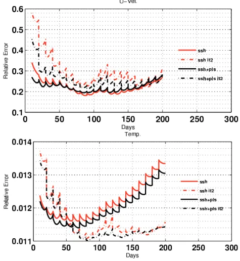
day of the experiment. . . 111 4.16 Relative errors of the zonal velocity (top) and the temperature (bottom)
for the experiments ssh 10d rd (red curve) and ssh 10d rd it2 (dashed red curve) and their equivalents with K constructed using PLS regression (black curves). . . 112 4.17 Figure shows the gradient of the cost function after each inner iteration
(left) and the reduction of the relative error for the zonal velocity for experiment ssh4j 10d rd uvt (right). . . 113 4.18 . . . 114 4.18 The figure shows errors of the SSH (a), the zonal velocity (b) and the
temperature (c). Each curve correspond to a different experiment, see table 4.5 for more details. . . 115 4.19 (a) RMS of vertical zonal velocity and first (b) and second (c) eof error
modes calculated using forecast from day 200 to day 720. . . 116 4.20 . . . 124 4.20 The panels represent the first four loading vectors of SSH used in the
calculation of the regression model between SSH and surface velocity. More specifically, they are the first four columns of the matrix PT. . . . 124
4.21 Vertical correlation of the modes presented in figure 4.20 with their re-spective modes at deeper layers. . . 125 4.22 Mean Squared error of the residuals (left panel) and R2score (right panel)
for the PLS algorithm using different number of modes, indicated in the legend, and for OLS. Results of fitting, i.e. the statistics are calculated using objects used in the construction of the regression model. . . 126
LIST OF FIGURES ix
4.23 Mean Squared error of the residuals (left panel) and R2score (right panel)
for the PLS algorithm using different number of modes, indicated in the legend, and for OLS. Results of prediction, i.e. the statistics are calcu-lated using objects not used in the construction of the regression model. 127
5.1 Top panels: Sea Surface Height (left) and Temperature profiles (right) observational network accumulated for a 2 days window. Bottom panels: Sea Surface Height (left) and Temperature profiles (right) observational network accumulated for 10 and 18 days window respectively . . . 134 5.2 SSH relative error for different assimilation windows and covariance rank.
Top left: rank(S) = 10. Top right: rank(S) = 30. Bottom left: rank(S) = 50. All experiments used ρ = 1, i.e. no covariance infla-tion is considered. . . 136 5.3 Zonal velocity relative error for different assimilation windows and
covari-ance rank. Top left: rank(S) = 10. Top right: rank(S) = 30. Bottom left: rank(S) = 50. All experiments used ρ = 1, i.e. no covariance inflation is considered. . . 137 5.4 Temperature relative error for different assimilation windows and
covari-ance rank. Top left: rank(S) = 10. Top right: rank(S) = 30. Bottom left: rank(S) = 50. Bottom right: rank(S) = 100. All experiments used ρ = 1, i.e. no covariance inflation is considered. . . 137 5.5 Initial condition relative error for the iterative Backward Smoother (iBS),
Back and Forth Kalman Filter (BFKF) and Running in Place (RIP). All experiments were initialized from climatological mean and covariance and use rank(S) = 20, Rssh = 0.08I and Rtemp = 0.5I. Dots represent
simulations performed using ρ = 1 and dashed line using ρ = 0.95. Top left: SSH; Top right: Zonal Velocity; Bottom: Temperature. . . 139
5.6 Initial condition relative error for the iterative Backward Smoother (iBS), Back and Forth Kalman Filter (BFKF) and Running in Place (RIP). All experiments were initialized from a mean and covariance calculated by the SEEK filter after its spin-up. rank(S) = 20, Rssh = 0.08I and
Rtemp = 0.5I. Dots represent simulations performed using ρ = 1 and
dashed line using ρ = 0.95. Top left: SSH; Top right: Zonal Velocity; Bottom panel: Temperature. . . 140 5.7 Figure shows the first seven Backward Smoother (iBS) iterations
initial-ized from a mean and covariance calculated by the SEEK filter after its spin-up. rank(S) = 20, ρ = 0.95 and Rssh = 0.08I, Rtemp = 0.5I. Left
panel: iterations from 1 to 7; Right panel: iterations from 8 to 15. . . 141 5.8 Figure shows the first seven Backward Smoother (iBS) iterations
initial-ized from a mean and covariance calculated by the SEEK filter after its spin-up. rank(S) = 50, ρ = 0.95 and Rssh = 0.08I, Rtemp = 0.5I. Top
left: iterations from 1 to 4; Top right: iterations from 5 to 10; Bottom panel: iterations from 11 to 15. . . 142 5.9 . . . 143 5.9 Histogram and negentropy calculated from the innovation sequence
avail-able for the data assimilation window over which the methods are iter-ated. (a) filter pass. (b) BFKF after 15 iterations. (c) iBS after 15 itera-tions. (d) RIP after 15 iteraitera-tions. rank(S) = 20, ρ = 1 and Rssh= 0.08I,
Rtemp = 0.5I. . . 144
5.10 Maximal and minimal principal angles between HSi and HSi+1
calcu-lated from the climatological initialization experiment for top panels: BFKF and bottom panels: RIP. Left panels: ρ = 1 and right panels: ρ = 0.95. . . 145 5.11 Sea Surface Height spread calculated for the iBS experiment initialized
from the climatological mean and covariance and employing ρ = 0.95. Left panel: after 5 iterations and Right panel: after 15 iterations. . . 146
LIST OF FIGURES xi
5.12 Maximal and minimal principal angles between HSi and HSi+1
calcu-lated from the filter initialization experiment for left panel: iBS and right panel: BFKF. Both using ρ = 0.95 . . . 147 5.13 Variation rate of the energy perturbations Ep = T1ln
kδx0k
kδxTk where k•k = R
Ω[ρ(u2+ v2) + ρg] dΩ, during the backward integrations of the iBS method.
Top left: rank(S) = 20 initialized from the climatological statistics; Top right: rank(S) = 20 initialized from the filter statistics; Bottom left: rank(S) = 50 initialized from the filter statistics; Bottom right: rank(S) = 100 initialized from the filter statistics. For all experiments Rssh= 0.08I, Rtemp = 0.5I and ρ = 1. . . 148
5.14 Initial condition relative error for the SEEK filter and smoother, the Backward Smoother (BS), the Back and Forth Kalman Filter (BFKF) and the BFKF but using a fixed basis (BFFKF) within the assimilation window. Top left: SSH error. Top right: zonal velocity error. Bottom: temperature error. All experiments were initialized from climatological mean and covariance and the filter parameters are rank(S) = 20, ρ = 0.95 and Rssh= 0.08I, Rtemp= 0.5I. . . 149
5.15 Initial condition relative error for the SEEK filter and smoother, the Backward Smoother (BS), the Back and Forth Kalman Filter (BFKF) and the BFKF but using a fixed basis (BFFKF) within the assimilation window. Top left: SSH error. Top right: zonal velocity error. Bottom: temperature error. All experiments were initialized from climatological mean and covariance and the filter parameters are rank(S) = 50, ρ = 0.95 and Rssh= 0.08I, Rtemp= 0.5I. . . 150
5.16 Mean forecast improvement calculated from the forecasts initialized from the BS and SEEK-smoo. Top left: SSH relative improvement. Top right: zonal velocity relative improvement. Bottom: temperature relative improvement. Positive (negative) values indicates the BS (SEEK-smoo) has better forecast performance. . . 152
List of Tables
2.1 Summary of the 4Dvar algorithm . . . 30
2.2 Summary of the Kalman Filter equations. . . 43
2.3 Summary of the fixed-lag Kalman smoother equations. . . 50
2.4 Summary of the SEEK filter and SEEK smoother equations. . . 52
2.5 Summary of the iBS algorithm using the SEEK filter for the analysis. The notation xi k|k,K indicates that we are referring to the iteration number i, that x is conditioned on all observations y1:K which is related with iterations it < i, but for the present iterations x is only conditioned on y1:k. The subscript k|k, K refers to a analysed state and k|k − 1, K to a forecast state. . . 58
2.6 Bayesian description of the Back and Forth Kalman Filter. . . 62
4.1 Summary of the experiments presented in section 4.6.1. The symbol ” xxd” states for the length of the data assimilation window in days, i.e. ssh 10d dd refers to an experiment assimilating SSH, using a 10 days DA window and default diffusion coefficients. In the table ”xx” may take the values: 2, 5, 10, 20 and 30. Two stop criterions are considered: a convergence criterion (ǫ = 0.5%), and 2 iterations. . . 86
4.2 Summary of the mean relative initial and final condition errors obtained from the DBFN experiments employing the reference diffusion and as-similating daily SSH observations. AW is the Assimilation window. e0 and ef are the mean initial and final errors, respectively. . . 98
4.3 Summary of the mean relative initial and final condition errors obtained from the DBFN experiments employing a reduced diffusion and assimi-lating daily SSH observations. AW is the Assimilation window. For each AW the top lines represent the experiments considering only 2 iterations and the bottom line the experiments considering ǫ = 0.0005. e0 and ef
are the mean initial and final errors, respectively. . . 99 4.4 Summary of the mean error growth rate obtained from the DBFN
ex-periments assimilating daily SSH observations. AW is the Assimilation window. For each AW the top lines represent the experiments considering the reference diffusion coefficient and the bottom lines the experiments considering a reduced diffusion coefficient. . . 102 4.5 Summary of the experiments presented in section 4.6.2. Two stop
crite-rions are considered: a convergence criterion (ǫ = 0.5%), and 2 iterations. 108 4.6 Summary of the mean relative error for the control experiment (Free),
the ordinary Nudging employing the PLS (Nudg+PLS), the DBFN em-ploying the PLS (DBFN+PLS) and the 4Dvar. . . 115
5.1 Summary of the mean relative initial condition errors obtained by the algorithms: SEEK filter, SEEK smoother, Backward Smoother (BS), Back and Forth Kalman Filter with Fixed basis (BFFKF) and the Back and Forth Kalman Filter (BFKF). Two reduced basis approximations are exploited one with rank 20 and another with rank 50. For each method the top lines are the mean relative errors calculated from day 1 to day 50, and the bottom lines the mean relative errors calculated from day 51 to 180. . . 151
LIST OF TABLES xv
Acronyms
BFN Back and Forth Nudging
BFFKF Back and Forth Fixed basis Kalman Filter BFKF Back and Forth Kalman Filter
BLUE Best Linear Unbiased Estimate BS Backward Smoother
DA Data Assimilation
DBFN Diffusive Back and Forth Nudging EKF Extended Kalman Filter
EnKF Ensemble Kalman Filter KF Kalman Filter
iBS iterative Backward Smoother LO Luenberger Observer
LQG Layered Quasi-Geostrophic
NEMO Nucleus for European Modelling of the Ocean OLS Ordinary Least Squares
PLS Partial Least Squares RIP Running in Place RM Regression Model(s)
SEEK Singular Evolutive Extended Kalman Filter SW Shallow Water
SSH Sea Surface Height
Abstract
Data Assimilation – DA – methods comprehend the ensemble of methods aiming to estimate the state of a system given all informations about it, i.e models and observations. Generally speaking, DA methods provide a way to weight the combination of models and observations. These methods are ex-tensively used in the generation of accurate initial conditions for atmospheric and oceanic forecast systems, as well as to produce reanalysis fields (past state reprocessing based on future observations). Their importance relies on the possibility of accurately predicting the future evolution of atmospheric and oceanic events, which would support decisions concerning the agriculture investments and natural hazards contention plans, for instance.
This thesis developed and implemented iterative data assimilation algo-rithms for a primitive equation ocean model, and compared them with other well established DA methods such as the 4Dvar and the Singular Evolutive Extended Kalman (SEEK) Filter/Smoother. The numerical model used was the NEMO model. It was configured to simulate a typical subtropical double gyre circulation at an eddy permitting resolution. The new proposed iterative algorithms, similarly to the Back and Forth Nudging, are all based on a se-quence of alternating forward and backward model integrations. Namely, they are the Backward Smoother (BS), which uses the backward model to freely propagate “future” observations backward in time, and the Back and Forth Kalman Filter, which also uses the backward model to propagate the obser-vations backward in time but, at every time an observation batch is available, an update step similar to the SEEK filter step is carried out. The Bayesian formalism was used to derive these methods, which means that they may be
used with any algorithm that estimates the a posteriori conditional probabil-ity of the model state by means of sequential methods.
The results show that the main advantage of the methods based on the BFN is the use of the backward model to propagate the observation informa-tions backward in time. By this way, it avoids the use of the adjoint model, needed by the 4Dvar, and of unknown temporal correlations, needed by the Kalman Smoother, to produce initial states or past model trajectories. The advantages of using the Back and Forth (BF) idea rely on the implicit use of the unstable forward subspace, which became stable when stepping back-wards, that allows the errors components projecting onto this subspace to be naturally damped during the backward integration. It was shown that fore-casts initialized from the Backward Smoother are 4-10% more accurate than the forecasts initialized by the SEEK Smoother using the same computational power. The BFN results are also encouraging when compared with the re-sults produced by a 4Dvar algorithm. Using prescribed weights along with climatological correlations between observed and non- observed variables, the BFN produced results which are at least comparable with the 4Dvar results but with 3 times less computational power.
Therefore, this work shows that there is a real interest in using the BF idea for producing initial condition states for ocean forecasts due to the simplicity of implementation of the backward model and due to the possibility of using existing softwares, which implement sequential DA algorithms, along with the Back and Forth iterations. Hence, it would be very simple to implement these new methods on the existing assimilation systems.
R´esum´e ´etendu
Cette th`ese a d´evelopp´e et mis en œuvre des algorithmes it´eratifs d’assimilation de donn´ees pour un mod`ele d’oc´ean aux ´equations primitives, et les a com-par´es avec d’autres m´ethodes d’assimilation de donn´ees bien ´etablies telles que le 4Dvar et le filtre/lisseur SEEK. Le mod`ele num´erique utilis´e est le mod`ele NEMO. Il a ´et´e configur´e pour simuler la circulation typique subtrop-icale en double gyre `a une r´esolution de m´eso´echelle (voir chapitre 3). Les nouveaux algorithmes it´eratifs propos´es, de fa¸con similaire au Nudging direct et r´etrograde, sont tout bas´es sur une s´equence d’int´egrations altern´ees du mod`ele direct et r´etrograde. Dans la pratique, les m´ethodes diff`erent quant `a la fa¸con dont les poids donn´es aux observations et au mod`ele sont calcul´es.
Nous mettons en ´evidence trois chapitres: l’un d´ecrivant les m´ethodes d’assimilation (chap. 2) et deux autres pr´esentant les r´esultats num´eriques (chap. 4 et 5). Dans le chapitre 2, les algorithmes ont ´et´e class´es comme des algorithmes d´eterministes, pour lesquels le syst`eme n’a pas de terme al´eatoire, et les algorithmes stochastiques. Pour les premiers, aucune con-dition d’optimalit´e n’a ´et´e utilis´ee pour calculer les gains, pour cette raison, nous avons continu´e `a appeler ces m´ethodes le Back and Forth Nudging (BFN), alors que pour les derniers, nous avons utilis´e les hypoth`eses de Kalman pour obtenir des gains optimaux.
Deux algorithmes, obtenus `a l’aide du raisonnement de Bayes et compte tenu d’un sc´enario de mod`ele parfait, ont ´et´e propos´es: le Backward Smoother (BS) et le Back and Forth Kalman Filter (BFKF). Le premier s’appuie sur la connaissance de la fonction de densit´e a posteriori finale, p(xK|y1:K), pour
r´ecup´erer la probabilit´e conditionnelle d’un ´etat pass´e ´etant donn´e les
vations pass´ees et futures, p(xk|y1:K) pour k < K. Dans la pratique, il int`egre
le mod`ele r´etrograde en utilisant la solution finale du filtre direct comme con-dition initiale. Il a ´et´e montr´e que lorsque la transition p(xK−1|xK) est connue
et lin´eaire dans les variables d’´etat, la solution du BS obtenue au temps tk
ini-tialis´ee `a partir de la solution du filtre de Kalman au temps tKest ´equivalente `a
la solution du lisseur de Kalman `a tk en utilisant les observations disponibles
jusqu’`a tK. Le deuxi`eme algorithme (BFKF) s’appuie formellement sur la
d´ecomposition des observations en p sous-ensembles ind´ependants, chacun d’eux ´etant assimil´e `a chaque nouveau passage du filtre. D’une mani`ere g´en´erale, il est tout `a fait semblable au BFN mais le gain K maximise la probabilit´e conditionnelle, p(xk|yn1:k) (pour le ni`eme passage du filtre direct)
ou p(xk|yk:Kn+1) (pour le ni`eme passage du filtre r´etrograde), `a chaque ´etape
d’analyse. La d´ecomposition d’observations ne fournit pas seulement un gain optimal, mais aussi un nombre optimal d’it´erations. Il est clair qu’en utilisant la mˆeme d´ecomposition d’observation pour le BS, celui-ci peut ´egalement ˆetre it´er´e.
Les chapitres 4 et 5 d´ecrivent les exp´eriences num´eriques r´ealis´ees avec ces m´ethodes. Dans le chapitre 4 l’approche d´eterministe a ´et´e utilis´e, ce qui sig-nifie qu’aucune condition d’optimalit´e n’a ´et´e consid´er´ee dans la construction des gains, tandis que dans le chapitre 5 le BS et le BFKF ont ´et´e utilis´es. Ind´ependamment de l’optimalit´e du gain, un probl`eme concernant les appli-cations oc´eaniques est la nature irr´eversible des mod`eles qui peuvent empˆecher l’utilisation du mod`ele r´etrograde.
Dans le chapitre 4, nous avons montr´e qu’il est impossible d’int´egrer le mod`ele r´etrograde sans un contrˆole rigoureux et un r´eseau d’observation irr´ealiste, mais que l’inversion du signe du terme de diffusion stabilise le mod`ele. Toute-fois, dans ce dernier cas, il a ´et´e observ´e une perte de pr´ecision, qui augmente avec la longueur de la fenˆetre d’assimilation. On a constat´e qu’il s’agissait d’un r´esultat de sur-diffusion, c’est `a dire que les champs sont fortement liss´es, ce qui ´equivaut `a une perte de la r´esolution effective du mod`ele.
LIST OF TABLES 5
de diffusion r´eduit offrant les plus petites erreurs. Nous avons trouv´e qu’avec un coefficient de diffusion constant (dans le temps et dans l’espace) les erreurs ont ´et´e r´eduites jusqu’`a une limite qui est li´ee `a la diffusion n´ecessaire pour stabiliser la m´ethode num´erique. Cela a ´et´e fait de mani`ere empirique, mais comme il a ´et´e sugg´er´e, cela peut ˆetre fait par la construction d’un op´erateur de diffusion d’ordre n qui fournit la r´eponse souhait´ee pour chaque ´echelle spatiale, c’est `a dire qui permet une bonne pr´ecision `a moyenne ´echelle tout en supprimant les instabilit´es num´eriques. Il s’agit clairement d’une question qui doit ˆetre ´etudi´ee.
Deux gains ont ´et´e test´es dans le chapitre 4, une matrice K diagonale, ce qui signifie que la covariance des erreurs sont ignor´ees et la dynamique du mod`ele lui-mˆeme propage les corrections vers les r´egions et les variables non observ´ees, et un K consistant en deux op´erations: d’abord les variables observ´ees sont mises `a jour en utilisant un poids prescrit, puis les variables non observ´ees sont mises `a jour en utilisant un mod`ele de r´egression. Comme notre objectif ´etait de construire une m´ethode peu coˆuteuse, le mod`ele de r´egression a ´et´e maintenu fixe pendant les cycles d’assimilation. Pour ce type d’utilisation, nous avons montr´e qu’une m´ethode de r´egression ayant des pro-pri´et´es de r´egularisation est pr´ef´erable. Dans ce travail, cette m´ethode est celle des moindres carr´es partiels. Elle cherche p directions dans l’espace d’observation et dans l’espace du mod`ele qui sont mieux corr´el´ees, en mˆeme temps qu’elles maximisent leur variances.
Ces deux gains ont ´et´e test´es avec diff´erents r´eseaux d’observations: un simulant les champs de SSH maill´es et un autre simulant les observations de SSH ´echantillonn´ees sur une piste typique d’un satellite altim´etrique. Les con-clusions que nous tirons de ce chapitre est que le mod`ele a une capacit´e limit´ee pour corriger les champs thermodynamiques lorsque seules les observations de SSH sont disponibles, et dans ce cas peu importe si la SSH maill´ee ou la SSH ´echantillonn´ee sur la trajectoire du satellite est assimil´ee. Plus les observa-tions sont rares, plus important est l’utilisation de mod`eles de r´egression pour aider le mod`ele `a diffuser les informations d’observations.
Enfin, il a ´et´e montr´e que, malgr´e la faible pr´ecision du mod`ele r´etrograde, lorsque le mod`ele de r´egression comprend toute la partie non observ´ee de l’espace d’´etat, notamment la temp´erature, le Diffusive Back and Forth Nudg-ing (DBFN) peut donner des r´esultats qui sont au moins ´equivalents au 4Dvar que nous avons utilis´e, mais avec un effort de mise en oeuvre beaucoup plus faible, car aucun code adjoint n’est n´ecessaire, et avec un coˆut de calcul pr`es de 3 fois plus faible. Remarquablement, le DBFN atteint leur niveau d’erreur asymptotique apr`es le premier cycle d’assimilation tandis que le 4Dvar et le Nudging direct ordinaire ont besoin de douze cycles.
Ce fait montre la puissance des it´erations `a r´eduire les erreurs lorsque l’´etat du mod`ele est tr`es diff´erent de l’´etat vrai, comme c’est le cas au d´ebut de l’exp´erience. Cet aspect a ´et´e discut´e dans la litt´erature par Kalnay and Yang (2010); Yang et al. (2012); Wang et al. (2013b) qui ont soulign´e l’importance des it´erations lorsque les non-lin´earit´es jouent un rˆole important et que les membres de l’ensemble ou de la base r´eduite n’engendrent pas le vrai espace d’erreur.
Dans le chapitre 5, le gain du BFN a ´et´e formellement d´eriv´e pour ˆetre le gain de Kalman standard. Dans ce cas, le filtre de rang r´eduit “ Singu-lar Evolutive Extended Kalman - filtre SEEK” a ´et´e utilis´e pour calculer les analyses. Le filtre SEEK et lisseur SEEK ainsi qu’une version it´erative de ce lisseur (Running in Place - RIP), semblable `a l’algorithme utilis´e par Kalnay and Yang (2010), ont ´et´e pris comme r´ef´erence.
Les r´esultats confirment que malgr´e la faible pr´ecision du mod`ele r´etrograde, il est avantageux de l’utiliser `a la place des corr´elations lin´eaires pour mettre `a jour un champ pass´e. Cela est dˆu `a la correction des composantes d’erreur qui se projettent sur le sous-espace instable au cours de l’int´egration r´etrograde. Ce m´ecanisme est particuli`erement important lorsque la base r´eduite couvre seulement un petit sous-espace instable, soit parce qu’il a un rang tr`es r´eduit ou parce que la base s’´etend sur les deux sous-espaces: instable et stable.
D’une part il a ´et´e montr´e que lorsque la matrice de covariance a un rang relativement grand (> 50) et engendre seulement un sous-espace instable,
LIST OF TABLES 7
les avantages de l’utilisation du mod`ele r´etrograde pour am´eliorer la solution de filtrage sont r´eduits. D’autre part, les pr´evisions initialis´ees apr`es une int´egration r´etrograde sont toujours am´elior´ees par rapport `a celles r´ealis´ees `a partir du filtre ou lisseur SEEK, en particulier dans la gamme de 10 `a 40 jours, mˆeme si les conditions initiales de ces derni`eres sont plus pr´ecises.
Si on est surtout int´eress´e par les conditions initiales pour des fins de r´eanalyse par exemple, une fa¸con possible de continuer `a am´eliorer les condi-tions initiales est de reproduire certains modes ”instables en r´etrograde/stables en direct“, ce qui empˆechera les erreurs qui se projettent sur ces modes de croˆıtre. Ceci implique une augmentation des coˆuts num´eriques, et donc ses b´en´efices doivent ˆetre soigneusement examin´es .
En ce qui concerne les versions it´eratives iBS, BFKF et RIP, l’am´elioration des variables non observ´ees est plus grande pour les deux premiers, tandis que pour les variables observ´ees les trois m´ethodes ont montr´e des performances similaires. Encore une fois, cela peut r´ev´eler l’importance de l’int´egration r´etrograde `a r´eduire les erreurs instables ainsi que r´ev´eler l’am´elioration de la covariance entre les variables observ´ees et non observ´ees. En outre, les it´erations ont transform´e la distribution des erreurs de pr´evision dans une dis-tribution plus gaussienne am´eliorant ainsi la performance du filtre/lisseur.
Une faiblesse d´etect´ee `a propos de notre mise en œuvre de l’iBS et BFKF est la divergence observ´ee lorsque l’ inflation a ´et´e consid´er´ee, mˆeme si nous avons vu que l’inflation fournit de petites erreurs en moins d’it´erations. Par cons´equent, nous sugg´erons l’utilisation de filtres qui n’ont pas besoin d’inflation ou de sch´emas d’inflation adaptatifs. Cela permettrait de conserver les statis-tiques de filtrage coh´erentes avec les statisstatis-tiques de l’erreur vraie et donc d’utiliser aussi efficacement que possible une observation particuli`ere, ´etant donn´e les limites de chaque m´ethode. En outre, les statistiques utilis´ees par l’ approche adaptative peuvent ˆetre utilis´ees pour obtenir un crit`ere d’arrˆet plus efficace, puisque le crit`ere de convergence que nous avons utilis´e dans le chapitre 4 n’est pas capable de d´etecter la divergence signal´ee dans le chapitre 5.
Cette th`ese a prouv´e qu’il existe un r´eel int´erˆet pour l’utilisation du DBFN et des algorithmes bas´es sur les it´erations du mod`ele direct et r´etrograde pour l’assimilation des observations oc´eaniques. Bien sˆur, il est n´ecessaire d’´etudier comment ces m´ethodes se comportent dans un syst`eme d’assimilation op´erationnel pour lequel, en g´en´eral, les mod`eles sont biais´es et pas parfaits. Plus de d´eveloppements sont n´ecessaires, notamment en ce qui concerne la diffusion de l’int´egration r´etrograde et la stabilit´e `a long terme des filtres/lisseurs qui peuvent ˆetre trait´es avec des syst`emes adaptatifs.
Enfin, nous croyons que les algorithmes pr´esent´es dans cette th`ese m´eritent d’ˆetre test´es en mode op´erationnel comme le sont le 4Dvar et les filtres de Kalman. En effet, compte tenu de la simplicit´e de mise en œuvre du mod`ele r´etrograde, les algorithmes it´eratifs pr´esent´es ici peuvent ˆetre facilement mis en œuvre en tirant partie des syst`emes d’assimilation existants.
Chapter 1
Introduction
1.1
Introduction (French)
La croissance de la population et la demande de plus en plus ´elev´ee de la protection sociale ont conduit `a une augmentation de l’exploitation des ressources naturelles. Les zones de forte concentration de population sont tr`es sensibles aux ph´enom`enes naturels extrˆemes. Elles sont d’une part directement affect´ees comme par exemple dans le cas du Tsunami qui s’est produit dans l’Oc´ean Indien en 2004 et celui du Japon en 2013, et d’autre part indirectement affect´ees en cons´equence des perturbations m´et´eorologiques sur la production alimentaire `a grande ´echelle.
Sur cette base, la connaissance des composantes du syst`eme physique de la Terre tels que l’atmosph`ere et l’oc´ean et des lois les r´egissant est devenue essentielle pour la vie moderne. La possibilit´e de reconstruire les ´ev´enements pass´es et de pr´edire avec pr´ecision les ´ev´enements futurs a chang´e la dynamique ´economique. Par exemple, les organismes d’assurance et de cr´edit ont eu recours `a la connaissance de la m´et´eo ainsi que des pr´evisions m´et´eorologiques pour ajuster leurs ´evaluations des risques.
Au cours des cinquante derni`eres ann´ees, des progr`es sur les pr´evisions m´et´eorologiques se sont produits en raison notamment de l’am´elioration de la formulation des mod`eles, comme une cons´equence du d´eveloppement impressionnant des ressources informatiques, et grˆace `a l’am´elioration des r´eseaux d’observation et des conditions initiales. Ce progr`es dans la pr´evision est illustr´ee `a la figure 1.1 par la qualit´e des pr´evisions des champs de 500hPa produites au NCEP1. La barre horizontale indique une augmentation d’un jour
1National Centers for Environmental Prediction
par d´ecennie dans la qualit´e des pr´evisions. Pour montrer que ceci est important pour la soci´et´e de nos jours, selon Ravinder Singh, chef de la physique agricole `a l’Institut indien de recherche agricole, ”la pr´ecision dans la pr´evision de la mousson peut aug-menter la production agricole de 10 pour cent `a 15 pour cent dans les zones pluviales “. Cela signifie que l’am´elioration des capacit´es de pr´evision repr´esenterait une croissance dans la production mondiale de nourriture.
Beaucoup moins d’attention a ´et´e accord´ee `a l’´elaboration des pr´evisions oc´eaniques. Toutefois, l’oc´ean joue un rˆole cl´e dans les r´egimes m´et´eorologiques et climatiques, car il d´elimite la basse atmosph`ere. A cette interface, il y a des ´echanges de quantit´e de mouvement, vapeur d’eau et de chaleur entre l’ocean et l’atmosph`ere. En outre, on pense que les interactions oc´ean-atmosph`ere deviennent un facteur dominant pour les pr´evisions `a long terme. Par exemple, les variabilit´es atmosph´eriques importantes, qui touchent directement plusieurs millions de personnes, telles que la mousson de l’oc´ean Indien et les ph´enom`enes El Nino/La Nina du Pacifique sont fortement contrˆol´ees par la dynamique de l’oc´ean sup´erieur (Keshavamurthy and Sankar Rao, 1992; Wang et al., 2012).
En outre, l’oc´ean et les r´egions cˆoti`eres sont des zones riches en ressources naturelles. Cela a conduit les ´etablissements humains `a se concentrer sur les zones `a proximit´e du littoral. A titre d’exemple, la densit´e populationnelle moyenne dans les r´egions cˆoti`eres a ´et´e estim´ee 3 fois plus ´elev´ee que la moyenne mondiale. De plus, les commerces `a travers le monde utilisent le plus souvent la mer `a l’exportation et `a l’importation des marchandises, et le poisson repr´esente environ un cinqui`eme des prot´eines animales dans l’alimentation humaine.
Par cons´equent, l’importance de produire des pr´evisions fiables de l’oc´ean et de l’atmosph`ere est justifi´ee, entre autres facteurs, par leur utilisation dans le soutien des activit´es ´economiques, ainsi que la gestion de l’environnement. Mais, quels sont les d´efis pour produire des pr´evisions fiables? En termes math´ematiques, une pr´evision est un probl`eme de valeur initiale. On nous donne un ensemble d’´equations diff´erentielles ´evolutives `a partir duquel nous voulons calculer l’´evolution de l’´etat du syst`eme, ´etant donn´e un ´etat initial. Par cons´equent, une bonne pr´evision d´epend du degr´e de repr´esentativit´e physique du mod`ele math´ematique (et num´erique) et du degr´e de pr´ecision des
condi-1.1. INTRODUCTION (FRENCH) 11
tions initiales.
Au d´ebut des ann´ees 60 le scientifique am´ericain Edward Norton Lorenz a d´eclar´e que la nature chaotique des ´equations r´egissant l’atmosph`ere impose une limite de pr´evisibilit´e de temps fini. Il a trouv´e qu’un mod`ele atmosph´erique simplifi´e initialis´e avec deux conditions initiales l´eg`erement diff´erentes entraˆıne deux solutions compl`etement diff´erentes apr`es une simulation sur deux semaines. Par cons´equent, beaucoup d’efforts ont ´et´e faits pour produire des conditions initiales les plus pr´ecises possible.
La science de la production de champs g´eophysiques pr´ecis a ´et´e nomm´e Assimila-tion de Donn´ees - DA (Bennett, 2002; Kalnay, 2003; Evensen, 2009). Ce nom vient du fait que les observations du syst`eme sont introduites (assimil´ees) dans les mod`eles pour am´eliorer les descriptions du syst`eme: l’observationnel et la math´ematique/num´erique. Cela signifie que l’assimilation vise `a fournir des informations sur le syst`eme r´eel qui sont en mˆeme temps plus proches de la v´erit´e que les observations et les mod`eles s´epar´ement. Pour illustrer les difficult´es rencontr´ees par l’assimilation de donn´ees oc´eaniques, les fig. 1.2 et 1.3 montrent un r´eseau d’observation typique de la mer M´editerran´ee et deux r´esultats de mod`ele pour la mˆeme r´egion, l’un avec une r´esolution spatiale de 12 km et l’autre de 3 km. Le premier aspect observ´e est la raret´e du r´eseau d’observation qui r´ev`ele que les observations ne sont pas assez denses pour produire des conditions initiales pour les mod`eles num´eriques. Plus que cela, il n’y a presque pas d’information directe sur la structure synoptique du champ vertical de masse (les balles vertes dans la figure repr´esentent les bou´ees Argo2). La plupart des donn´ees sont des mesures directes3 de la
surface de l’oc´ean (temp´erature de surface de la mer et hauteur de la surface de la mer), mˆeme s’ils peuvent observer des propri´et´es associ´ees `a la dynamique de la thermocline (Wunsch, 1997).
L’Assimilation de Donn´ees a fait ses d´ebuts sur la base de deux piliers: la th´eorie du contrˆole (Jazwinski, 1970; Gelb, 1974) et la th´eorie du contrˆole optimal (Lions, 1971). Ces domaines sont particuli`erement int´eress´es par le contrˆole de syst`emes ´electriques et de trajectoire balistique et satellitaire, par exemple. De ces deux branches scientifiques ont ´emerg´e les m´ethodes d’assimilation de donn´ees les plus utilis´ees de nos jours: le Filtre 2Sondes robotiques oc´eaniques d´eploy´es dans le monde entier. Les sondes flottent aussi profond que 2 km et une
fois tous les 10 jours ´echantillonnent mesures de conductivit´e et de temp´erature de la colonne d’eau. Les donn´ees sont transmises aux scientifiques `a terre par satellite. (source http://en.wikipedia.org/wiki/Argo %28oceanography% 29)
3
Cela ne signifie pas que les mesures ont ´et´e faits in situ , mais que les propri´et´es mesur´ees sont `a la surface ou est la surface elle-mˆeme.
de Kalman (Kalman, 1960; Kalnay, 2003; Evensen, 2009) et les m´ethodes variationnelles en quatre dimensions (Le Dimet and Talagrand, 1986; Bennett, 2002). Toutefois, en raison de la taille tr`es importante des probl`emes et des ressources informatiques limit´ees, l’assimilation de donn´ees a eu son d´ebut, au milieu des ann´ees 70, avec l’utilisation de m´ethodes simples et peu coˆuteuses, parmi lesquelles se distingue le Nudging.
La m´ethode du Nudging est bas´ee sur le deuxi`eme axiome de Newton et consiste `a ajouter un terme de for¸cage dans le second membre d’un syst`eme donn´e, afin de pousser doucement le mod`ele vers une valeur prescrite. La premi`ere apparition du Nudging dans la litt´erature g´eophysique a ´et´e en 1974 (Anthes, 1974). Dans ce travail, les auteurs ont propos´e d’utiliser le Nudging pour att´enuer les probl`emes d’initialisation des mod`eles atmosph´eriques.
La premi`ere apparition d’une application r´eussie du Nudging en oc´eanographie a ´et´e en 1992 dans une ´etude qui a assimil´e la hauteur de la mer, issue de mesures satellitaires, dans un mod`ele quasi-g´eostrophique en couches (Verron, 1992). Depuis, la m´ethode a ´et´e appliqu´ee avec succ`es `a plusieurs probl`emes oc´eanographiques tels que les conditions aux limites (Marchesiello et al., 2001; Chen et al., 2013), downscaling (Li et al., 2012), et d’autres probl`emes d’assimilation de donn´ees (Verron, 1992; Haines et al., 1993; Lewis et al., 1998; Killworth et al., 2001; Thompson et al., 2006). En ce qui concerne les applications aux probl`emes d’assimilation des donn´ees, les poids attribu´es au mod`ele et aux observations, en g´en´eral, ne repose sur aucune condition d’optimalit´e, mais sont plutˆot des scalaires ou des fonctions Gaussiennes construites sur la base des hypoth`eses physiques. Les points forts de cette m´ethode sont la simplicit´e de mise en œuvre dans les mod`eles num´eriques complexes, la faible demande de puissance de calcul et la r´egularit´e temporelle de la solution.
La disponibilit´e croissante de la puissance de calcul a permis l’utilisation de m´ethodes d’assimilation de donn´ees plus avanc´ees. En g´en´eral, ces m´ethodes reposent sur l’utilisation d’informations sur les statistiques des erreurs du mod`ele et des observations pour pond´erer la combinaison mod`ele-observations. Deux de ces m´ethodes qui sont largement utilis´ees par les centres de pr´evision sont le filtre de Kalman d’ensemble-EnKF (Evensen, 1994) et ses variations (Pham, 2001; Hunt et al., 2007), et les m´ethodes variationnelles en quatre dimensions-4Dvar (Le Dimet and Talagrand, 1986; Courtier et al., 1994). Pour
1.1. INTRODUCTION (FRENCH) 13
la premi`ere, les coˆuts de calcul sont dˆus `a la propagation de l’ensemble, g´en´eralement form´e par des centaines de membres, pour calculer la pr´evision. Pour la seconde, les coˆuts sont dˆus `a la n´ecessit´e de minimiser une fonction coˆut dans un tr`es grand espace d’´etat (108 variables). Cela peut demander plusieurs it´erations de l’algorithme de
min-imisation, ce qui en pratique se traduit par plusieurs int´egrations des mod`eles directs et adjoints.
Cependant, mˆeme avec l’int´erˆet croissant pour ces techniques complexes construites sur des arguments th´eoriques solides, le Nudging n’a pas ´et´e laiss´e de cˆot´e. Des travaux r´ecents ont utilis´e le Nudging avec des m´ethodes plus avanc´ees telles que l’interpolation optimale (Clifford et al., 1997; Wang et al., 2013a), l’EnKF (Ballabrera-Poy et al., 2009; Bergemann and Reich, 2010; Lei et al., 2012; Luo and Hoteit, 2012), 4DVAR (Zou et al., 1992; Stauffer and Bao, 1993; Vidard et al., 2003; Abarbanel et al., 2010) ou les filtres particulaires (Luo and Hoteit, 2013; Lingala et al., 2013) pour extraire le meilleur de chaque m´ethode. Dans le cas particulier de l’hybridation avec l’EnKF propos´e par Lei et al. (2012), l’algorithme r´esultant a l’avantage de la propagation dynamique de la ma-trice de covariance `a partir de l’EnKF et utilise le Nudging pour att´enuer les probl`emes li´es `a l’intermittence de l’approche s´equentielle, qui entre autres choses entraˆıne le rejet possible de certaines observations.
R´ecemment, Auroux and Blum (2005) ont revisit´e la m´ethode du Nudging et ont propos´e un nouvel algorithme appel´e Back and Forth Nudging (BFN). Le BFN con-siste en une s´equence d’int´egrations des mod`eles direct et r´etrograde, tous les deux en utilisant un terme de rappel aux observations, comme pour le Nudging direct. Le BFN int`egre le mod`ele direct vers l’arri`ere dans le temps en ´evitant la construction de l’adjoint et/ou des mod`eles lin´eaires tangents (n´ecessaire par le 4Dvar et les filtres ´etendus). Par cons´equent, il n’utilise que le mod`ele non lin´eaire pour propager des informations vers l’avant et vers l’arri`ere dans le temps. Le gain du Nudging r´etrograde, qui a un signe oppos´e par rapport au Nudging direct, a un double rˆole: pousser le mod`ele vers les observations et stabiliser l’int´egration r´etrograde, ce qui est particuli`erement important lorsque le mod`ele n’est pas r´eversible.
La performance du BFN dans les applications num´eriques en utilisant une vari´et´e de mod`eles, y compris les mod`eles non-r´eversibles, tels que le mod`ele de Saint-Venant ou
un mod`ele multi-couche quasi-g´eostrophique, ainsi qu’un mod`ele atmosph´erique `a haute r´esolution, sont tr`es encourageants (Auroux, 2009; Boilley and Mahfouf, 2012). De plus, en utilisant un gain scalaire simple, le BFN a produit des r´esultats comparables `a ceux obtenus avec le 4Dvar, mais avec un coˆut de calcul inf´erieur (Auroux, 2009; Auroux et al., 2012).
L’objectif principal de cette th`ese est de mettre en œuvre le BFN pour un mod`ele d’oc´ean aux ´equations primitives et de comparer sa performance avec celles des fil-tres/lisseurs de Kalman et du 4Dvar. En outre, nous avons utilis´e la th´eorie de l’estimation bay´esienne pour construire des gains optimaux pour le BFN. En utilisant les hypoth`eses de Kalman (`a d´efinir) nous avons deriv´e le Backward Smoother et sa version it´erative, ainsi que le Back and Forth Kalman filter (Cosme, personal communication) qui peut ˆetre vu comme une extension du BFN pour les syst`emes stochastiques.
Le mod`ele num´erique utilis´e est NEMO (Madec (2008)), actuellement utilis´e par le centre fran¸cais de pr´evision de l’oc´ean, MERCATOR (http://www.mercator-ocean.fr/fre), pour produire et livrer des pr´evisions oc´eaniques. La configuration du double tourbillon id´ealis´ee `a une r´esolution ”eddy permiting” est utilis´e. Cette configuration pr´esente l’avantage d’ˆetre simple du point de vue de la g´eom´etrie et du for¸cage, mais avec toutes les caract´eristiques des processus de m´eso-´echelle d’un ocean de latitude moyenne.
Cette th`ese est organis´ee comme suit :
• Le chapitre 2 pr´esente les aspects th´eoriques concernant les m´ethodes d’assimilation de donn´ees utilis´ees dans la th`ese. L’accent est mis sur leurs diff´erences, car il va permettre l’analyse des r´esultats num´eriques produits.
• Le chapitre 3 pr´esente le mod`ele num´erique et ses approximations. Les aspects de la mise en œuvre du mod`ele r´etrograde sont ´egalement pr´esent´es. Enfin, la mise en place des exp´eriences, en ce qui concerne ses conditions initiales et aux limites, la param´etrisation sous-maille et les champs de for¸cage, est d´ecrite.
• Le chapitre 4 pr´esente une ´etude approfondie du BFN appliqu´e `a un mod`ele d’oc´ean aux ´equations primitives et compare les r´esultats avec ceux produits par un algo-rithme 4Dvar.
1.1. INTRODUCTION (FRENCH) 15
Smoother et le Back and Forth Kalman filter. Leur performance est compar´ee avec la performance d’un filtre de Kalman et d’un lisseur de Kalman.
• Enfin, le dernier chapitre pr´esente les conclusions et les perspectives d’avenir con-cernant le BFN et le Back and Forth Kalman Filter.
1.2
Introduction
Over the last century, the populational growth and the increasing demand for social wel-fare has led to an increasing exploitation of natural resources. Large clusters of human settlements have proved to be very sensitive to extreme natural phenomenas, being on the one hand directly affected as for example in the case of 2004 Indian Ocean tsunami and 2013 Japan tsunami, and on the other hand indirectly affected as a consequence of weather perturbations on the large scale food production.
Based on this, the knowledge of the Earth’s physical system components such as the atmosphere and the ocean and their governing laws has become essential for sustaining the modern way of life. The possibility of reconstructing past events and accurately predict future events has changed the economic dynamics. For example, insurance and credit agencies have been using the knowledge about the weather as well as weather predictions to adjust their risk assessments.
In the last fifty years, progress on weather forecasting occurred especially due to improvements in the models formulation, as a consequence of the impressive develop-ment of computational resources, as well as due to improved observational networks and initial conditions. This progress in forecasting is illustrated in Figure 1.1 by skill of the 500 hPa forecasts produced at the NCEP4. The horizontal bar indicates an
one-day-per-decade increase in forecast skill. To show how important this can be for the nowadays society, according to Ravinder Singh, head of agricultural physics at the In-dian Agricultural Research Institute, ”Precision in the monsoon forecast can raise farm production by 10 percent to 15 percent in rainfed areas”. This means that improving forecast capabilities would represent increasing the world food production.
Much less attention has been given to the development of ocean forecasts. However, the ocean plays a key role in the weather and climate regimes since it bounds the lower atmosphere. At this interface, the ocean and the atmosphere exchange momentum, heat and water vapor. Furthermore, it is believed that ocean-atmosphere interactions become a dominant factor at long forecast ranges. For example, important atmospher-ical variabilities, which directly affect several millions of people, such as the Indian’s monsoon and the pacific El Nino/La Nina phenomena are in high degree controlled by
4
1.2. INTRODUCTION 17
the upper ocean dynamics (Keshavamurthy and Sankar Rao, 1992; Wang et al., 2012).
Figure 1.1: Skill of the 36 hour (1955–2004) and 72 hour (1977–2004) 500 hPa forecasts produced at NCEP. Forecast skill is expressed as a percentage of an essentially perfect forecast score. Extracted from Lynch (2008).
Moreover, ocean and coastal regions are natural resource-rich areas. This has led Human settlements to focus on near-coastal areas. As an example, the average popula-tional density in coastal regions was estimated 3 times higher than the global average. In addition, worldwide trades mostly use the sea to export and import goods as well as fish account for roughly one fifth of all animal protein in the human diet.
Therefore, the importance of producing reliable forecasts of the ocean and the atmo-sphere is justified by, among other factors, their use in supporting economic activities as well as the environmental management. But, what are the challenges for producing reliable forecasts? In mathematical terms, a forecast is an initial value problem, i.e. we are given a set of evolutive differential equations from which we want to calculate the system state evolution given an initial state. Therefore, a good forecast depends on how representative of the real physics the mathematical (and numerical) model is and how accurate the initial conditions are.
In the beginning of the 60’s the American scientist Edward Norton Lorenz stated that the chaotic nature of the governing equations imposes a finite time predictability limit. He founded that starting a simplified atmospheric model with slightly different initial conditions resulted in two completely different fields after two weeks simulation. Consequently, much more effort has been made for producing initial conditions as
ac-curate as possible.
The science of producing accurate geophysical fields has been named Data Assimila-tion - DA (Bennett, 2002; Kalnay, 2003; Evensen, 2009). This name comes from the fact that observations of the system are introduced (assimilated) into the models to improve both descriptions of the system: the observational and the mathematical/numerical. It means that assimilation aims to provide informations about the real system which are at the same time closer to the truth than observations and models separately.
To exemplify the challenges faced by ocean data assimilation, Figs.1.2 and 1.3 show a typical Mediterranean Sea observational network and two model outputs for the same region, one with a spatial resolution of 12km and the other of 3km. The first observed aspect is the observational network sparsity that reveals that the observations are not dense enough to produce initial conditions for numerical models. More than this, there is almost no direct information about the synoptic vertical mass field structure (the green bullets in the figure represent Argo5 drifters that sample the water column every
10 days). Most of the data are direct6 measurements of the ocean surface (sea surface
temperature and sea surface height), even though they may ”observe“ thermocline-related motions (Wunsch, 1997).
Figure 1.2: Typical Mediterranean Sea observational network for a 10day time window.
The model outputs (Fig. 1.3), in their turns, reveals that changing the model resolu-5Argo consists of a large collection of small, drifting oceanic robotic probes deployed worldwide. The
probes float as deep as 2 km. Once every 10 days, the probes surface, measuring conductivity and tem-perature profiles to the surface. The data are transmitted to scientists on shore via satellite. (source http://en.wikipedia.org/wiki/Argo %28oceanography%29)
6
1.2. INTRODUCTION 19
tion alters the large scale features. This may be the impact of a poor representation of the sub-grid scale process, i.e. the parametrization of the non-modeled physics. How-ever, models provide continuous fields which at some extent reproduce the underlying physics. Hence, DA methods may be seen as methods to interpolate the observations using the model as the interpolation function.
Figure 1.3: Surface velocity for experiments employing the same forcing fields but on the right using spatial resolution of 1.7km (Glazur64) and on the left of 7km (MED16). Figures adapted from Duchez (2011).
The DA science had its beginning based on two pillars: the control theory (Jazwin-ski, 1970; Gelb, 1974) and the optimal control theory (Lions, 1971). These domains are especially interested in the control of electric systems, ballistic and satellite trajectory, for instance. From these two scientific branches emerged the nowadays most used data assimilation methods: the Kalman Filters (Kalman, 1960; Kalnay, 2003; Evensen, 2009) and the four dimensional variational methods (Le Dimet and Talagrand, 1986; Bennett, 2002). However, due to the very huge size of the problems and the limited computa-tional resources available, data assimilation had its beginning, in the mid-70s, with the use of simple and inexpensive methods, among which stands out the Nudging.
The well-known Nudging method is based on the Newton’s second axiom and con-sists in adding a forcing term in the right hand side of a given system in order to gently push the model toward a prescribed value. The first appearance of Nudging in the geophysical literature was in 1974 (Anthes, 1974). In this work the authors proposed to use nudging to mitigate initialization problems in atmospheric models.
The first appearance of a successful application of Nudging to oceanographic DA was in 1992 in a work that assimilated sea surface height derived from satellite measurements into a quasi-geostrophic layered model (Verron, 1992). Since then, the method has been successfully applied to several oceanographic numerical problems such as boundary con-ditions (Marchesiello et al., 2001; Chen et al., 2013), downscaling (Li et al., 2012), and other DA problems (Verron, 1992; Haines et al., 1993; Lewis et al., 1998; Killworth et al., 2001; Thompson et al., 2006). With respect to applications to DA problems, the weights given to the model and the observations are in general not based on any op-timality condition, but are rather scalars or Gaussian-like functions constructed based on physical assumptions. The appeals of this method are the simplicity of implementa-tion in complex numerical models, the low computaimplementa-tional power required and the time smoothness of the solution.
The increasing availability of computing power has allowed the use of more advanced data assimilation methods. In general, these methods rely on the use of information about the model statistics and observations errors to weight the model-observations combination. Two of these methods that are widely used by prediction centers are the ensemble Kalman filter- EnKF (Evensen, 1994) and its variations (Pham, 2001; Hunt et al., 2007), and the four dimensional variational method 4Dvar (Le Dimet and Ta-lagrand, 1986; Courtier et al., 1994). For the first, the numerical costs are due to the propagation of the ensemble, usually formed by hundreds of members, to calculate the forecast. For the second, the costs are due to the need of minimizing a cost function in a very huge state space (108 variables). This may require several iterations of the
minimization algorithm, which in practice requires several integrations of the direct and adjoint models.
However, even with the growing interest in these complex techniques built on solid theoretical arguments, nudging has not been left aside. Recent works have used nudg-ing along with more advanced methods such as Optimal interpolation (Clifford et al., 1997; Wang et al., 2013a), EnKF (Ballabrera-Poy et al., 2009; Bergemann and Reich, 2010; Lei et al., 2012; Luo and Hoteit, 2012), 4Dvar (Zou et al., 1992; Stauffer and Bao, 1993; Vidard et al., 2003; Abarbanel et al., 2010) or particle filters (Luo and Hoteit, 2013; Lingala et al., 2013) to extract the best of each method. In the particular case of
1.2. INTRODUCTION 21
the hybridization with the EnKF proposed by Lei et al. (2012), the resulting algorithm takes the advantage of the dynamical propagation of the covariance matrix from EnKF and uses nudging to mitigate problems related to the intermittence of the sequential ap-proach, which among other things entails the possible discarding of some observations. Recently, Auroux and Blum (2005) revisited the Nudging method and proposed a new algorithm called Back and Forth Nudging (BFN). The BFN consists in a sequence of forward and backward model integrations, both of them using a feedback term to the observations, as in the direct nudging. The BFN integrates the direct model backwards in time avoiding the construction of the adjoint and/or tangent linear models (needed by the 4DVar and extended filters). Therefore, it uses only the fully non-linear model to propagate information forward and backward in time. The nudging gain, which has an opposite sign with respect to the forward case, has a double role: push the model toward observations and stabilize the backward integration, which is especially important when the model is not reversible.
The BFN performance in numerical applications using a variety of models, including non-reversible models such as a shallow water model and a multi-layer quasi-geostrophic model as well as a high resolution atmospherical model, are very encouraging (Auroux, 2009; Boilley and Mahfouf, 2012). Moreover, using a simple scalar gain, it produced results comparable to those obtained with 4DVar but with lower computational require-ments (Auroux, 2009; Auroux et al., 2012).
The main objective of this thesis is to implement the BFN for a primitive equation ocean model and to compare its performance with Kalman filters/smoother and the 4Dvar. In addition, we used the Bayesian estimation theory to construct optimal gains for the BFN. Using the Kalman’s hypotheses (to be defined latter) we derived the Back-ward Smoother and its iterative version as well as the Back and Forth Kalman Filter (Cosme, personn. communication) that can be seen as BFN extensions for stochastic systems.
The numerical model used is NEMO (Madec (2008)), currently used by the french ocean forecast center, MERCATOR (http://www.mercator-ocean.fr/fre), to produce and deliver ocean forecasts. The well-known idealized double gyre configuration at eddy-permitting resolution is used. This configuration has the advantage of being
sim-ple from the geometry and forcing point of view but with all the mid latitude ocean mesoscale process features.
This thesis is organized as follows:
• Chapter 2 introduces the theoretical aspects regarding the data assimilation meth-ods used in the thesis. The focus is on their differences, as it will feed the discussion of the numerical results produced.
• Chapter 3 presents the numerical model and its approximations. Aspects of the backward model implementation are also presented. Finally, the experiment set-up regarding its initial and boundary conditions, subgrid-scale parametrization and forcing fields is described.
• Chapter 4 presents a comprehensive study of the BFN applied for a primitive equation ocean model and compares the results with those produced by a 4Dvar algorithm.
• Chapter 5 presents an implementation of two “new” smoother algorithms: the Backward Smoother and the Back and Forth Kalman Filter. Their performance are compared with a Kalman Filter and a Kalman Smoother performance.
• Finally, the last chapter presents the conclusions and future prospects concerning the BFN and the Back and Forth Kalman Filter development.
Chapter 2
Data Assimilation Methods
Contents
2.1 Introduction . . . 24 2.2 Preliminary Concepts . . . 24 2.3 Four Dimensional Variational Method - 4Dvar . . . 27 2.4 The Back and Forth Nudging . . . 30 2.4.1 Forward Nudging . . . 30 2.4.2 Backward Nudging . . . 33 2.4.3 Iterating the Forward and the Backward Nudging . . . 34 2.5 Bayesian Estimation . . . 37 2.5.1 Kalman Filter . . . 39 2.5.2 Kalman Smoothers . . . 47 2.5.3 Iterative Kalman Smoothers . . . 56 2.5.4 Probabilistic Four Dimensional Variational Method . . . 62 2.6 Numerical Implementation . . . 63 2.6.1 D-BFN . . . 63 2.6.2 Kalman Filter/Smoothers . . . 63 2.6.3 4Dvar . . . 64 2.7 Conclusions . . . 64 23