Giant Planets
Texte intégral
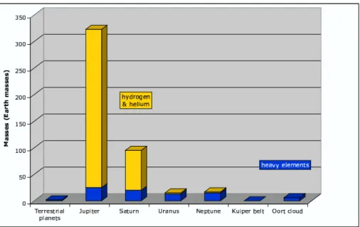
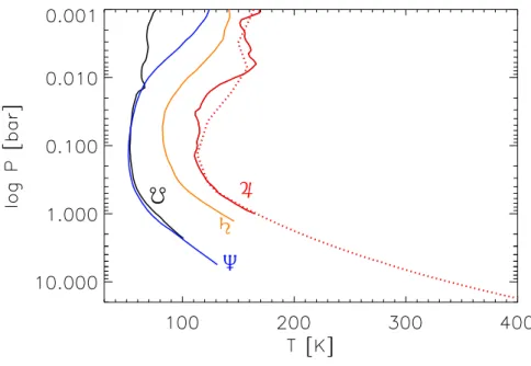
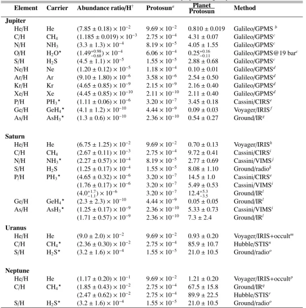
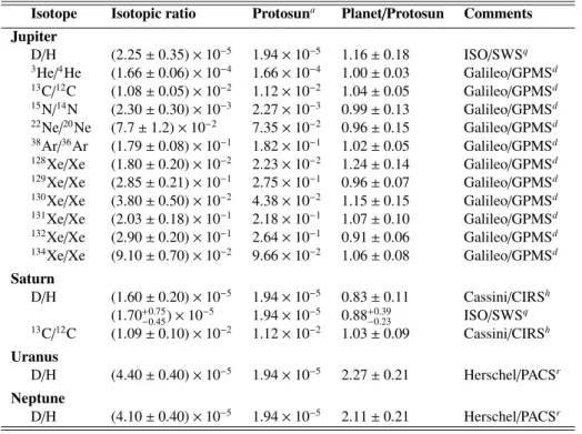
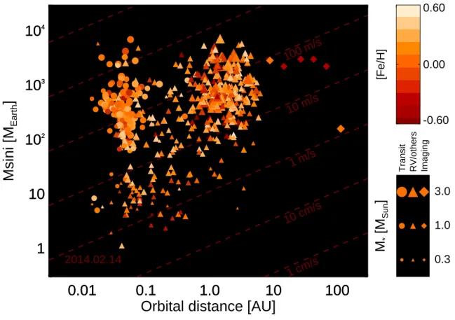
Figure
Documents relatifs
An overview of the Baikal region small mammal diversity from the Late Pliocene to Pleistocene shows that during the Late Pliocene and Early Pleistocene several common species
L’archive ouverte pluridisciplinaire HAL, est destinée au dépôt et à la diffusion de documents scientifiques de niveau recherche, publiés ou non, émanant des
P. antarcticum is an important prey of several fish species.. antarcticum et d’autres familles de poissons antarctiques récoltés dans la même zone d’étude. antarcticum
We observed functional variations in her Toll like 5 receptor (TLR 5) gene and two coagulation variations (Tissue Factor (TF) 603 and Plasminogen-Activator-Inhibitor-1 (PAI-1)
Ocean time-series of genomic data have been expanding rapidly (e.g., Bermuda Atlantic Time Series, http://bats.bios.edu/; Integrated Marine Observing System,
(2019) An association between maternal weight change in the year before pregnancy and infant birth weight: ELFE, a French national birth cohort study.. This is an open access
The same behavior as in the “full data” case is observed with an approximate 3 dB performance loss between the calibrated and DI-uncalibrated scenarios, and no estimation possible
Jewel bearings for wafches and sundry industries Steine für Uhren und verschiedene Industrien Piedras para la relojeria e industrias diversas.
