The Boston Seaport : an economic analysis of large scale urban redevelopment on adjacent residential real estate values

(1)

-j

The Boston Seaport: An Economic Analysis of Large Scale Urban Redevelopment on Adjacent Residential Real Estate Values

By

Samuel Philip Weissman B.S., Business Administration

Boston University Boston, Massachusetts (2013)

Submitted to the Department of Urban Studies and Planning and Center for Real Estate in partial fulfillment of the requirements for the degree of

Master in City Planning and

Master of Science in Real Estate Development at the

MASSACHUSETTS INSTITUTE OF TECHNOLOGY June 2018

The author here by grants to MIT the permission to reproduce and to distribute publicly paper and electronic copies of the thesis document in

whole or in part in any medium now novwn or)ereafter created.

Author

Signature redacted

Samuel Philip Weissman Department of Urban Studies and Planning Center for Real Estate May 21, 2018 Certifie4-b

Accepted by_

Accepted by

Signature redacted

Professor Albert Saiz Daniel Rose Ass rofessor of Urban Economics and Real Estate Thesis Supervisor

Signature redacted _____

7----Professor of Practice Caesar McDowell Chair, MCP Committee Department of Urban Studies and Planning

Signature redacted

Professor Albert Si

ITUTE Daniel _{Associate Professor of Urban Economics and Real Estate}

]

epartment of Urban Studies and Planning & Center for Real Estate MASSACTUSML NST_{OF TECHNOLOGY}

JUN 18 2018

(2)

(3)

The Boston Seaport: An Economic Analysis of Large Scale Urban Redevelopment on Adjacent Residential Real Estate Values

by

Samuel Philip Weissman

Submitted to the Department of Urban Studies and Planning and Center for Real Estate on May 21, 2018 in partial fulfillment of the

requirements for the degree of Master in City Planning and Master of Science in Real Estate Development

ABSTRACT

This paper develops a Repeat-Sales Price Index on an unbalanced panel of residential real estate properties. Facilitated by price index creation, this study analyzes the change in housing price levels in South Boston, Massachusetts over the period of time of a major adjacent redevelopment, The Seaport. The main purpose is to determine the effect of large scale urban redevelopment projects on adjacent housing prices over time. Using comprehensive residential sales data from The Warren Group, this paper offers an analytical tool that can be utilized by stakeholders such as policy makers, investors, developers and homeowners. It informs a deeper understanding of the

potential effects of large scale redevelopment on affordable housing and gentrification, investment returns, urban land theory and homeowner equity. During the study period from 1996 - 2017, results show that South Boston housing in the "Closest to the

Seaport Redevelopment" distance quartile range earned an additional 6.21% in annual price growth than South Boston housing in the "Furthest from the Seaport

Redevelopment" distance quartile range. This result is compared with a composite Boston housing benchmark of 15 zip codes (excluding South Boston and The Seaport). Results demonstrate that South Boston residential real estate located closer to the Seaport grew a total of 130% more than South Boston residential real estate located further away from 1996 - 2017, statistically significant with 95% confidence.

Thesis Supervisor: Albert Saiz

Title: Daniel Rose Associate Professor of Urban Economics and Real Estate, Director of Center for Real Estate

(4)

Acknowledgements

I would like to thank my thesis advisor Albert Saiz and thesis reader Walter Torous, for their advice and insight.

I would like to thank Alex van de Minne and Andrea Chegut for their expertise in price index creation and Laura Krull for her assistance with ArcGIS.

(5)

affordability, which serves as an input to decisions regarding affordable housing development and inclusionary zoning policy. For investors, a price index can provide data on property price changes, act as a benchmark for the market and assist in honing property modeling assumptions. For homeowners, a price index can shed light on how their home equity, and therefore household wealth, has changed over time. For academics, price indices can prove useful in comparing real estate across geographies and to other financial asset classes.

This study analyzes the ex-post price reaction of residential properties in the South Boston neighborhood to the adjacent massive redevelopment of the South Boston Waterfront known as "The Seaport" project. Over the period of redevelopment, South Boston housing prices soared. Based on the data utilized for this thesis, simple median housing prices grew 495%, from $105,000 in 1996 to $627,000 in 2017, or nearly 24% annualized. However, this simple median does not tell the whole story as it does not control for quality of housing or distance from the redevelopment.

Through the construction of a transaction-based Repeat-Sales price index, this study measures the change in residential properties at various distances from The Seaport from 1996 - 2017, controlling for property quality. This exercise attempts to yield the true change in home price levels over the period and isolate the

redevelopment effect on price. This is performed by focusing on properties not involved in the redevelopment, rather those in close proximity to The Seaport. As the majority of redevelopment activity occurred after 2010, the period of 1996 - 2017 provides adequate pre- and post-redevelopment pricing context.

(7)

Area of Study

The neighborhoods referenced repeatedly throughout this thesis are: 1.

2.

The Seaport

South Boston Residential

The Seaport is the area which has been recently redeveloped over the period from 1996-2017 and includes the Seaport and Fort Point neighborhoods.

The South Boston Residential neighborhood is the primarily residential section south of the Seaport Waterfront/Fort Point area which this study hypothesizes has seen significant increases to its real estate values due to the redevelopment of The Seaport.

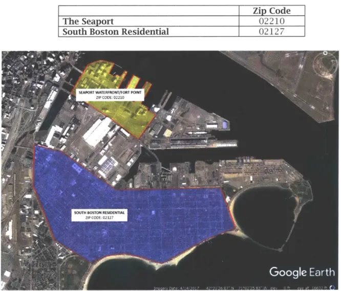
Zip Code Demarcations

Zip Code

The Seaport 02210

South Boston Residential 02127

~j~jfl~

(8)

The Seaport History and Redevelopment

In the 1 9th and early _{2 0}th century, the Seaport served predominantly as a bustling

industrial hub in South Boston. Fan Pier earned its name from the large train yard on the site, in which the trains fanned out towards the water. The Fort Point area to its south was developed in the mid-19th century by a single developer, The Boston Wharf Company, to create warehouses and wharves. By the 1990's, much of the land in the Seaport was vacant and primarily devoted to parking lots (save for vacant Fort Point Warehouses). However, Boston was emerging as a first-tier city and thus the area was ripe for redevelopment.

From 2000 to 2017, the Seaport District in Boston gained over 11 million square feet of new development and more than 4,000 new residents (NEBS 2016). A massive amount of private and public investment facilitated this process with direct project investment of over $2.2 billion and government investment of more than $18 billion (Boston Globe 2017, BidUp 2017). As of February 2017, average market-rate residential asking prices in the Seaport were $1,498 per SF, greater than most other high-end Boston neighborhoods: North End Waterfront ($996), Back Bay ($1,472) and Beacon Hill ($1,413) (Acitelli 2017). The Seaport neighborhood character has completely changed from abandoned rail yards and parking lots to a mixed-use district of glass and steel class A office towers, high-end experiential retail and luxury high-rise housing.

(9)

The Seaport Redevelopment Documentation

ftwM mu - y ,f nfl -m m ₀

Figure 2: The Seaport 1981 -Source: Boston Globe (2017)

(10)

2. LITERATURE REVIEW

This literature review is divided into two sections; a discussion of literature surrounding urban land economics and real estate within the context of the Seaport redevelopment and a discussion of the various methodologies and data types for price index creation.

Discussion 1: Urban Land Economics and Real Estate Value:

In William Alonso's 1960 seminal text, A Theory of the Urban Land Market, he details the fundamental theories of real estate value and urban land markets. Alonso augments David Ricardo's (1817) agricultural theory of land rent to explain the modern urban land market.

At its simplest, Alonso's Monocentric City model explains that a location's value is based on the level of transportation costs associated with that location relative to a single central node. In Alonso's work, this central node is represented by the Central Business District (CBD) of a city where jobs are located and all workers must commute to daily. It follows that properties located a further distance from the CBD will be associated with higher transportation costs to the center (in both time and money) than those located closer. Thus in general, households with greater willingness-to-pay for a central location, to avoid commuting, will outbid those with less willingness-to-pay, causing central locations to have higher land value than less central locations.

This model has been critiqued by Wheaton (1979) and Berry and Kim (1993) for being too simplistic in its assumptions of a single employment center, where all

workers travel the same direction and transportation costs are the only location consideration factor for households.

(11)

However, this thesis suggests that the confluence of a few unique factors lead a modified version of Alonso's theory to be applicable to the Seaport redevelopment. Alonso's theory operates primarily under the post-war suburbanization paradigm of a suburban households commuting in to a central employment hub. However, this paradigm has shifted in recent years. The New Urbanist/Smart Growth movements, codified in the Ahwahnee Principles (1991), have promoted ideas of high-density, walkable/transit-oriented, mixed-use urban neighborhoods, which have been developed in cities all over the United States. As of 2014, 62% of the Millennial

Generation, born 1982 - 2004 (Bump 2014), prefer to live and work in walkable mixed-use neighborhoods in cities rather than suburbs (Nielsen 2014). If central employment node is replaced with "central mixed-use node", Alonso's model appears to apply.

The Seaport redevelopment, colloquially known as a "Live-Work-Play"

environment, is specifically designed to provide high-density amenities to encourage workers to live, work and shop in the same place. Within the small community of

South Boston, The Seaport redevelopment has likely emerged as the new central

mixed-use node, given South Boston's small size, primarily residential use and extreme proximity to the redevelopment. Therefore, instead of seeing the Seaport as only South Boston's employment node, it is rather viewed as the location where South Boston residents want to pursue all activities (live, work, shop, dine). Given the new social preference to locate in these mixed-use environments, individuals with the highest willingness-to-pay will choose to live closer to the Seaport to reduce transportation costs to all of their daily activities, rather than only work. Those individuals will bid up the more central land values, while South Boston land further away will have lower value.

(12)

Discussion 2: Methodologies and Data Types for Price Index Creation This thesis relies on the Repeat-Sales Index methodology and the transaction data for index creation. The following section will discuss other methodologies and forms of data, the reasons behind not pursuing those in this study and discuss both the merits and limitations of the chosen methodology and data type.

Mean or Median Pricing Index Methodology

A very simplified methodology for creating a price index relies on using annual mean or median housing transaction prices. However, by utilizing these simple

summary statistics, the index cannot control for quality and characteristics of housing sold in each period. Therefore, this method cannot successfully determine the actual changes in house price level from changes in quality of property.

Hedonic Pricing Index Methodology

The Hedonic Pricing regression methodology (Rosen 1974, Fisher et al. 1994) seeks to control for housing quality by determining the effect of each attribute of a housing unit on its total value, for example the value of each additional bedroom, bathroom, swimming pool, building age, location, square footage, etc. However, performing this analysis at the zip code level requires an immense amount of data which details all major attributes of every housing unit. The transaction data set utilized for this thesis did not contain housing unit attributes and thus the Hedonic

Pricing methodology could not be performed. The lack of comprehensive data on housing attributes is not new or unique to this study and has hindered the

(13)

Repeat-Sales Pricing Index Methodology

Bailey, Muth and Nourse first put forward the methodology for creating a Repeat-Sales price index for real estate in their 1963 landmark paper, further

developed by Case and Shiller (1987). A major concern in determining the change in housing price level in a geographic area is the fact that housing is a heterogeneous good. Each housing unit has a unique set of attributes, which make comparing the values of housing units to each other challenging. The advantage of the Repeat-Sales index methodology is its ability to control for the quality of housing, substantially reducing the amount of data needed to create an accurate price index. This method relies on comparing the value within an existing unit to itself over time as it transacts, to gain an understanding of value change over time. This also allows for the creation of a housing price index without the granularity of gathering and then determining the value of each attribute within each housing unit. The economic model created in this thesis utilizes the Repeat-Sales index methodology.

Limitations of Repeat-Sales Methodology

While the Repeat-Sales methodology's power lies in its simplicity, its simplicity also contributes to its limitations. First, the Repeat-Sales method only captures real estate that has transacted at least twice during the period of analysis. This reduces the sample size of data in the index by excluding the housing that transacts only once over the study period, effectively omitting the market information those sales

communicate.

Secondly, the Repeat-Sales methodology assumes that quality of housing is controlled for. However, unless specifically identified and removed, properties used in a repeat-sales index may have capital improvements or renovations performed, simply

(14)

due to the nature of long periods of time between sales of a property. While Case & Shiller (1987) had sufficient data in their study to identify and remove housing which had quality changes, the data used for this thesis did not provide that type of

information. Thus this index has the potential for bias if two purported identical properties are compared, when in reality a capital improvement has been performed. Thus, the embedded price change that is due to the improvement is obscured and unable to be separated from the actual house price level change.

Assessment-Based Indices

Annual time-series assessment values for all properties in Suffolk County are available on the City of Boston Tax Assessor websitel dating back to 1985 for many residential properties. This data thus covers a longer period of time than the study period (1996 - 2017), which could have added more clarity to the model. However, despite the ready availability of this data, the decision was made to utilize market sales transaction value data instead of tax assessment value data. The is decision was made primarily to avoid appraisal error and subjectivity.

The City of Boston Property Tax Facts & Figures Fiscal Year 2018, specifies that it bases property tax values on "full and fair cash value" which an owner would be willing to accept and a buyer willing to pay on the open market. However, there is a

significant research to support the theory that assessed value is often disconnected from true fair market value and not in a predictable manner. Clapp and Giaccotto (1991) point out that it is "well known that the property tax assessor measures

property values with error" and wrote a paper on methods of dealing specifically with

(15)

this issue in creating assessed-value price indices. In contrast, fair market value by definition is determined by the actual price paid in the market, thus transaction data acts as an unbiased barometer of the market at any given time.

Furthermore, in most cities, a homeowner has the right to appeal their "over-valued" property assessment with their municipality and if successful, have it lowered. To do so, the homeowner must prove using comparable properties that their home was miss-assessed by the municipality. While it seems that this process would have the effect of "correcting" the assessment data, it is not performed uniformly by all owners. Appealing property assessments take time, money, the requisite knowledge and/or a lawyer and therefore owners will not uniformly appeal but only rather owners with the ability to do so. It is unable to be determined by analyzing the assessment data which properties have been re-assessed which thus, creates an inconsistent data set.

Appraisal-Based Indices

Appraisal-Based Indices are those that are based on property appraisals

performed by independent appraisers or often by brokers. Similar to assessed values, appraised values are subject to error and subjectivity by the appraisers. Furthermore, the creation of indices with appraisal data can cause Index Smoothing. Index

smoothing occurs when the true volatility of index is smoothed out, thus understating property risk. Quan and Quigley (1991) highlight that appraisal indices exhibit

considerable smoothing due to their valuation methods which base updated appraisals on "a mixture of previous appraisals, 'new' comparable property information and current market information". Thus the intent of using transaction based data is to display the true movement of property prices.

(16)

Research Hypothesis

Based on the modified Alonso's Monocentric City Model, discussed in the literature review, I posit that South Boston residential real estate that is located closer to the Seaport redevelopment will have exhibited higher growth in value over the study period (1996 - 2017) than South Boston residential real estate located further away. This hypothesis relies on the theory that within the South Boston neighborhood, the Seaport redevelopment has emerged as the central mixed-use node where all

households locating in the area, with a high willingness-to-pay, desire to locate close to.

If my hypothesis is correct, we would expect to see higher price index levels in the real estate located closer to the Seaport over the redevelopment period and lower in the real estate located further away. Furthermore, this difference would be

(17)

3. DATA

Consolidated comprehensive real estate sales transaction data can often be difficult to obtain. Thus, the data utilized in this thesis is provided by the Warren Group, a provider of real estate and financial information since 1872. The data

provided is real estate transaction data from 1996 through 2017 for all Suffolk County properties in Massachusetts. It includes 175,413 unique properties and 786,547

recorded transactions for all property types. However, the data subset utilized for this study is only residential property types in the 02127 zip code.

The data columns utilized relevant to the Repeat-Sales model generated are:

property ID; building address; unit number; sales price; transaction date; zip code; latitude; longitude and city

South Boston Residential (02127) - Annual Sales

Volume ($)

.

11

MMM0

1iiII

0 0 0 MMM0 0 0 0 - 4 r- r- NJ N N4 N1 IZIt Lfl I' (N N~ r-0 0 rN

I

00

0

0 '-I N M Ln 1.0 r-0 0 0 0 0 0 0 0 N N1 Nq N Nq N N N

Figure 4: South Boston Annual Sales Volume -Source: Warren Group, Samuel Weissman (2018) $450,000,000 $400,000,000 $350,000,000 $300,000,000 $250,000,000 $200,000,000 $150,000,000 $100,000,000 $50,000,000 _j

(18)

South Boston Residential (02127) - Annual Transaction Volume

I

w-

III

M0O 0 -4 NI Mf C*j Ln LO r- 00 M 0 M~ M~ 0 0 0 0 0 0 0 0 0 0 -i M~ M~O 0 0 0 0 0 0 0 0 0 0 0 v--i r- .-f N N NI N Nq Nq N N N N4 N o o o o o o o N - N I M LN N N1

Figure 5: South Boston Annual Transaction Volume -Source: Warren Group, Samuel Weissman (2018) 900 -800 -2 700 -a 600 -0 500 -0 4-0-0 -300 -z 200 -100 -0-

I

(19)

4. ESTIMATION STRATEGY

The Repeat-Sales price index employed in this study utilizes an Ordinary Least Squares (OLS) regression on an unbalanced panel. While Bailey et al (1963) utilize only pairs of sales, in reality individual properties may transact more than twice over the course of the period of study. Since the South Boston dataset was in fact an

unbalanced panel of properties transacting at various frequencies, this study utilizes the Grimes and Young (2010) Repeat-Sales Unbalanced Panel method which is designed to apply all sales transactions of each property rather than splitting sales into pairs. In this method, log price is regressed on set time fixed-effects and property fixed-effects. The estimation model is:

In

Pit

= ai

+

pt

+

Eit

Where:

In

Pit

is the log price of property i in year t at represents the individual property fixed-effect

pt

represents the time fixed-effect (to create log price index)

Eit is a residual

To account for distance, the properties were divided into four bins based on individual distance from a selected "central point of redevelopment" in the Seaport. The regression above was generated four separate times for each distance bin.

(20)

5. METHODOLOGY

This thesis utilizes a Repeat-Sales on an unbalanced panel methodology to create a price index for South Boston Residential.

Software Usage

The modeling aspect is aided by the use of several software programs. Particularly, Microsoft Excel for data filtering, clean up and analysis preparation, RStudio statistics software for regression analysis and ArcGIS geographic software for mapping, geocoding and creating distance variables.

Data Preparation

The Suffolk County historic sales transaction dataset provided by the Warren Group is imported into excel and filtered based on Zip Codes: 02127 - South Boston Residential. The data is then filtered to only include the following property codes:

* 1-4 Fam Res; 1-Fain Res; 2-5 Fam Res; 2-Fam Res; 3-Fam Res; 4-8 Unit Apt; 9+ Unit Apt; Apt Bldg; Condominium; Resid-Other; and Res-Mtl Bldg

All mortgage refinancing activities are removed from the dataset. All residential sales values below $10,000 are considered nominal sales and removed from the

dataset. Date in the format YYYYMMDD is converted to a Year format YYYY. The PropID column in the Sales dataset is compared with the PropID Assessment Values

dataset which contains latitude and longitude information. This is merged into the Sales dataset to facilitate geocoding. The data is sorted by PropID and then by Year to ensure that each individual property's transactions are adjacent to each other in the

(21)

dataset in chronological order. All properties (PROPID) with only a single transaction in the data are removed due to the necessity of repeated purchase and subsequent sale per PROPID to perform the index creation. A column is calculated for the log of the price as an input into the regression.

Geocoding and Distance Variable Creation

The following steps are performed separately for the South Boston residential dataset in ArcGIS. Utilizing the latitude and longitude data gathered during data preparation, each property is geocoded as a point on a map of Massachusetts. For

South Boston Residential, the District Hall (42.3 5209, -71.0454761) landmark is selected as the central location of the Seaport Redevelopment which all South Boston Residential distances would be measured from. This is the central node of Seaport Square, which is the area of the Seaport that has experienced the most redevelopment activity. The "Generate Near" data analysis tool is utilized to measure the distance from each point to its respective central redevelopment location. The distance

reported is a Geodesic distance, which is a Euclidian distance but of a curved surface, thus taking into account the curvature of the earth. The output of this activity created the distance variable utilized in the Repeat-Sales regression analysis.

Repeat-Sales Index Creation

The Repeat-Sales regression analysis is performed on the South Boston

residential dataset in RStudio. The dependent variable, log price, is regressed against independent variables, time fixed-effect (Year) and property fixed-effect (PROPID). The effect of distance is captured by separating properties into four distance bins, based

(22)

on each property's distance from The District Hall Landmark and then broken into quartiles.

Property Distance from Number of Number of

District Hall Transactions Properties

First Quartile 0.7701<Dist.<=1.1159 miles 3,032 1,135

Second Quartile 1.1159<Dist.<=1.2811 miles 3,034 1,115

Third Quartile 1.2811<Dist.<=1.4255 miles 3,052 1,111

Fourth Quartile 1.4255<Dist.<=1.8943 miles 3,038 1,128

A Repeat-Sales index was then created by running four Ordinary Least Squares (OLS) unbalanced panel regressions, one for each distance quartile for the period of

1996 - 2017. This yields four indices that explain price changes for each distance from the District Hall "center of redevelopment".

(23)

Map Output from Distance Quartile Geocoding

*

10 010 4bC Closest (0.7701<x<1.1159 mi)

* Second Closest (1.1159<x<=12811 mi)

C C

Second Furthest (1,2811<x<=1.4255 mi)

Furthest (1.4255<x<=1.8943 mi)

Figure 6: Map Output from Distance Quartile Geocoding - _{Source: Warren Group Data, Samuel Weissman (2018)}

w

C C

(24)

Statistical Significance Test

To determine if the difference between South Boston properties closest to District Hall in the Seaport and those furthest, a 95% confidence (+/- 1.96 std. error) interval is applied to the mean of the last four years of data (2014, 2015, 2016, 2017) on the log coefficients and standard errors. A more detailed discussion follows in the Results section.

All Boston (Benchmark)

As a benchmark, the South Boston residential data is compared to a composite indicator of 15 Boston zip codes, excluding South Boston and the Seaport. The All Boston (benchmark) dataset is made up of 42,335 transactions and 14,609 unique properties. The following neighborhoods and zip codes are captured:

# Zip Neighborhood

1 02108 Beacon Hill

2 02110 Downtown Crossing/Financial District

3 02114 West End 4 02113 North End

5 02109 Faneuil Hall/North End 6 02111 Chinatown/Tufts 7 02116 Back Bay 8 02118 South End 9 02115 Fenway 10 02215 Kenmore 11 02199 Roxbury 12 02129 Charlestown 13 02120 Mission Hill 14 02119 Roxbury 15 02124 Dorchester

(25)

6. RESULTS

South Boston Residential Repeat-Sales Price Index, 1996 - 2017

800 - _-Closest _{to Seaport (0.7701 < x <= 1.1159 mi)}

-Second Closest to Seaport (1.159 < x <= 1.2811 mi)

700 - Second Furthest from Seaport (1.2811< x <= 1.4255 mi) Furthest from Seaport (1.4255 < x <= 1.8943 mi)

=- eAll Boston (Benchmark)

600 500-400 4 - - p 300goOww 200 -100

(26)

The output of the model clearly demonstrates that all South Boston residential real estate saw tremendous growth in values over the study period of 1996 - 2017. The closest South Boston residential real estate to Seaport ("Closest") grew 758% while the furthest South Boston residential real estate from the Seaport ("Furthest") grew 628% and All Boston (benchmark) residential grew 508% over the same period.

Impact of the Great Financial Crisis

Results clearly show the effect of the Great Financial Crisis and recession (December 2007 - June 2009) as all but the Second Furthest from the Seaport experienced negative growth during 2008 and every distance category experienced negative growth during 2009 (BLS 2012). Interestingly, the Closest seems to have been affected more by the recession than the Furthest, declining 11.68% in 2008 and 4.24% in 2009 vs. the Furthest declining 2.87% in 2008 and 2.36% in 2009. A potential cause of this difference might be the Closest proximity to a risky development project with its future in jeopardy during the financial crisis years.

Statistical Significance

Using an average of the last four years (2014, 2015, 2016, 2017), the difference between Closest and Furthest was found to be statistically significant at a 95%

confidence interval (+/- 1.96 SE). An average of the last four years was used to show a cumulative statistical significance trend rather than selecting an individual year, in which significance may vary given market volatility. However, the Second Closest and

Second Furthest were not found to be statistically significantly different than the Closest at a 95% confidence interval. Second Closest is significant only with 8.76% confidence and Second Furthest is significant with 66.795% confidence.

(27)

Examination of Closest vs. Furthest Soo - i _{Closest to Seaport (0.7701 <}_x_<=

1.1159 mi)

700 Furthest from Seaport (1.4255 < x <= 1.8943 mi)

mm= eAll Boston (Benchmark)

600

500

400

200

-100

Figure 8: South Boston Price Index, Closest/Furthest, 1996-2017 -Source: Warren Group Data, Samuel Weissman (2018)

Given the statistical significance between Closest and Furthest at 95%, the relationship was further examined. Between 1996 and 2000, the Closest and Furthest moved closely together and by 2000, the Closest index level was only 7.16% higher than the Furthest. However, in 2001 and 2002, the growth in Closest began to outpace the Furthest and by 2002 the Closest had increased 54.60% more than the Furthest

since the base year. This period from 2000-2002 is of particular importance given that it coincides with the delivery of the first major redevelopment activity: Seaport Hotel (1998), Seaport East (2001) and Seaport West (2002), Boston Convention and Exhibition Center (under construction during 2002). This effort delivered a combined 2.2 million SF of office/retail, a 426-room hotel and 2.1 million SF of convention and exhibition

(28)

space. From this point through the end of the study period, the narrowest gap achieved in any given year between Closest and Furthest was 49.19% in 2003.

Over the 21-year study period, the Closest increased 130.34% more than the Furthest. As a benchmark, the Closest increased 2 52.29% more than All Boston (benchmark), a 12.01% annualized growth rate. The Furthest increased 121.95% more than All Boston (benchmark), a 5.81% annualized growth rate.

This indicates that South Boston residential real estate located in the 0.7701 -1.116-mile range from the Seaport redevelopment earned an additional 6.21% in annual price growth versus South Boston residential real estate located in the 1.426 -1.895-mile range.

Given an average value of Closest South Boston residential in 1996 of $92,678 and 758% growth over the study period, each house gained roughly $609,821 to an

average price in 2017 of $702,499. In aggregate across all 1,135 Closest properties in the database, $692,146,835 of value was created from 1996 - 2017.

(29)

Decile Testing

Further examination of the results is performed by breaking the data into distance deciles and comparing the first decile and tenth decile. As can be seen in the plot below, South Boston residential real estate in the first decile (x<=.9512 miles from Seaport) grew 951% over the study period, while South Boston residential real estate in the tenth decile (1.584<x<=1.894 miles from Seaport) grew only 664%. This represents an average added price growth of 13.7% annually to the first decile above the tenth decile. This result further supports the hypothesis that being closer to the Seaport had a positive impact on price growth.

Figure 9: First Decile vs. Tenth Decile, 1996-2017 -Source: Warren Group Data, Samuel Weissman (2018)

900 800 700 600 500 400 300 200 1n ===First Decile -Tenth Decile

100,

'\ 0 CP

6P

-P

N -; -

-6 16P r6p rf

-V 4 4 4

(30)

7. IMPLICATIONS

This study has far reaching implications for many different stakeholders including investors, homeowners and policy makers. While there are other Boston housing price indices available, such as the S&P CoreLogic Case-Shiller Boston Home Price NSA Index, none available get to the level of granularity of this study for South Boston. Although it is useful to observe and understand city-wide house price changes, that data is slightly irrelevant for describing the situation within any one isolated neighborhood. This thesis essentially provides bespoke housing data to stakeholders

at the South Boston community-level. At a higher level, it yields the relative locational value difference that a major mixed-use redevelopment has on adjacent housing.

Investment

From an investment perspective, this study provides this study confirms the age-old real estate adage "location, location, location". However, rather than simply implying the somewhat obvious assumption that real estate closer to a desirable

location is more valuable, this study quantifies the additional gain to real estate in The Seaport context. This can serve as a benchmark for residential investment in other areas close to redevelopment projects.

Furthermore, the results suggest that there exists a spatial bounds or "sweet spot", within which real estate is affected by redevelopment and where beyond it may not be. This distance can serve as a filter for informed investment decision in the future.

(31)

Policy

From a Boston-wide policy perspective, affordable housing is a major ongoing concern. Expenditures on housing were far and away the single largest category of annual household expenditures in Boston in 2015-16 at 39.2% of total annual

expenditures; 6.3% higher than the national average and 26.8% higher than the second largest category of spending in Boston, transportation (BLS 2016).

40-0 39.2

35.0 32.9 United States n Boston

30.0 25.0 20-0 _16.4 15.0 ₁₂₄ _{11.6 12.1} 12.6 11.2 10.0 79 6.4 5.1 5.1 3 . 0.0 Z.6

Housing T n iottation Personal Food Heathwre Enterbinmeft Cash Education

nsuranoa and Ontrbutions

pensiona

Figure 10: Percent distribution of average annual expenditures for major categories in the United States and Boston,

2015-2016 -Source: U.S. Bureau of Labor Statistics (2016)

This thesis demonstrates the effect of the Seaport redevelopment, which was city approved, on surrounding residential real estate values and thus on affordability at the neighborhood level. The model can be used not necessarily to predict, but rather to inform the policy around major redevelopment of other areas for example, the proposed Suffolk Downs redevelopment and East Boston Residential.

(32)

Potential Application: Suffolk Downs Redevelopment Case Study

4NO

Figure 11: HYM Suffolk Downs Master Plan Rendering -Source: HYM (2017)

On November 30th, 2017, the HYM Investment Group filed a Project Notification Form (PNF) with the Boston Planning and Redevelopment Agency to re-develop the 161-acre former East Boston race track, Suffolk Downs. The project calls for 11 million square feet of mixed-use development completed in multiple phases over the two decades (HYM 2017). As of 2017, HYM's plan mimics what has been built in the

Seaport since 2000, down to the number of potential square feet. Furthermore, HYM's renderings have a similar look and density to the Seaport and HYM even participated in the development of luxury apartments Waterside Place Phase 1A completed in the Seaport in 2014. Due to the similarities between South and East Boston, The Seaport

(33)

Repeat-Sales price index may shed light on future changes in East Boston residential due to the Suffolk Downs redevelopment.

Figure 12: Suffolk Downs Site and East Boston Residential- Source: Google Earth, Samuel Weissman (2018)

East and South Boston Comparison

East Boston residential real estate surrounds the Suffolk Downs site and exhibits comparable characteristics to South Boston residential prior to the

redevelopment of the Seaport, particularly with respect to demographics, industry, neighborhood character and property types. The neighborhoods both occupy

waterfront land along the Charles River and Atlantic Ocean. The majority of housing stock is stick frame or low-rise brick. Both neighborhoods are/were made up of

primarily working-class immigrants. Both areas have pockets of heavy industrial uses, South Boston's shipping, fish processing, iron and glass works, Con-Edison power

(34)

plant and East Boston's shipbuilding hub and Logan Airport. While the Seaport as a whole is much larger than Suffolk Downs, the majority of development as of 2017 has been focused in Seaport Square and Fort Point, an area of roughly 170 acres, not incomparable to Suffolk Down's 161 acres.

Potential Limitations of the Comparison

The major difference between South Boston and East Boston is the connection to the rest of Boston. Prior to the 2006 completion of the Central Artery/Tunnel Project sinking of 1-93 interstate underground, known as "The Big Dig", South Boston and East Boston were both disconnected from Boston. South Boston separated from the rest of Boston by the massive 1-93 highway and East Boston separated by the

Atlantic Ocean. After the project, South Boston was completely accessible, by all modes of transit, as an extension of Downtown Boston, whereas the Atlantic Ocean will always remain a physical barrier to the extension of Boston's activity into East Boston. While in reality, the Blue Line MBTA train only takes three minutes (Google 2018) to traverse the one-mile distance across the ocean gap from Maverick Station in East Boston to Aquarium Station in Downtown Boston, the psycho-geographic barrier of the ocean is

likely to affect East Boston in a way that South Boston is not.

Regardless of the limitations of the comparison, this thesis can be utilized to understand how East Boston residential real estate values may change over the period

of development of Suffolk Downs and this knowledge can be employed in policy decisions around affordable housing in the neighborhood. Potential applications include first, forecasting the affordable housing needs that would proliferate if East

(35)

subsidy programs to incentivize developers to build affordable housing before this value uplift occurs.

(36)

8. CONCLUSION

This thesis creates a price index for South Boston residential to expose the change in housing price levels over the period 1996 - 2017. This study confirms that over the Seaport redevelopment period, South Boston residential real estate located closer to the Seaport exhibited marked growth in value above and beyond South Boston residential real estate. South Boston residential real estate "closest to the Seaport" grew 758% over the period while real estate "furthest from the seaport" grew 628%, representing an average of 6.21% per year additional gain to the closest real estate.

While it cannot be definitively confirmed that the Seaport redevelopment was the sole cause for this higher price growth, there does appear to be a significant correlation. Of course, there are many other important physical and social factors which affect residential real estate values such as proximity to transit nodes, neighborhood amenities, walkability, crime/safety, quality of schools and general perception. Yet, it appears that the enormous scale of major redevelopment activity in the Seaport has in fact affected adjacent residential real estate in a positive manner.

Future research into this area may attempt to include the additional variables listed above to increase the explanatory power of the model. Moreover, incorporating data on major renovations, possibly through matching properties to building permit data, would significantly improve model accuracy by filtering out transactions which have had substantial upgrades performed.

(37)

9. BIBLIOGRAPHY

1. Acitelli, Tom. "Amazon Picks the Boston Area as One of 20 Finalists to Host Second Headquarters - Curbed Boston," 2017.

https://boston.curbed.com/2018/1/18/16905130/amazon-picks-boston.

2. "Curbed Cup Elite Eight: (16) Downtown Crossing vs. (8) Seaport District." Curbed Boston, December 18, 2017. https://boston.curbed.com/2017/12/18/16787492/curbed-cup-downtown-crossing-seaport-district.

3. "East Boston's Major New Developments, Mapped." Curbed Boston, October 10, 2017. https://boston.curbed.com/maps/east-boston-new-developments.

4. "Suffolk Downs Redevelopment Could Go One of Two Ways." Curbed Boston, December 6, 2017.

https://boston.curbed.com/boston- development/2017/12/6/16739398/suffolk-downs-redevelopment-amazon-construction.

5. "Waterfront vs. Seaport: How Their Prices Compare." Curbed Boston, February 16, 2017.

https://boston.curbed.com/2017/2/16/14628628/boston-real-estate-waterfront-seaport.

6. Alonso William. "A Theory of the Urban Land Market." Papers in Regional Science 6, no. 1 (January 14, 2005): 149-57. https://doi.org/10.1111/J.1435-5597.1960.tbOl710.x. 7. Arizona State University. "The Ahwahnee Principles I The Codes Project," 1991.

http://codesproject.asu.edu/node/65.

8. Arribas-Bel, Daniel, and Fernando Sanz-Gracia. "The Validity of the Monocentric City Model in a Polycentric Age: US Metropolitan Areas in 1990, 2000 and 2010." Urban

Geography 35, no. 7 (October 3, 2014): 980-97.

https://doi.org/10.1080/02723638.2014.940693.

9. BPDA. "Development Projects I Boston Planning & Development Agency," 2018. http://www.bostonplans.org/projects/development-pjrojects.

10. "Suffolk Downs I Boston Planning & Development Agency," 2018.

http://www.bostonplans.org/projects/development-projects/suffolk-downs. 11. "Timeline I Boston Planning & Development Agency," 2018.

http://www.bostonplans.org/about-us/timeline.

12. Bump, Philip. "Here Is When Each Generation Begins and Ends, According to Facts." The

Atlantic, March 25, 2014. https://www.theatlantic.com/national/archive/2

014/03/here-is-when-each-generation-begins-and-ends-according-to-facts/359589/.

13. Bureau, US Census. "Wealth, Asset Ownership, & Debt of Households Detailed Tables: 2013." Accessed April 13, 2018.

https://www.census.gov/data/tables/2013/demo/wealth/wealth-asset-ownership.html. 14. Case, Karl, and Robert Shiller. "Prices of Single Family Homes Since 1970: New Indexes

for Four Cities." Cambridge, MA: National Bureau of Economic Research, September 1987. https://doi.org/10.3386/w2393.

(38)

15. CBPP. "Chart Book: The Legacy of the Great Recession." Center on Budget and Policy Priorities, August 5, 2010. https://www.cb-pp.org/research/economy/chart-book-the-legacy-of-the-great-recession.

16. Chegut, Andrea M., Piet M. A. Eichholtz, and Paulo Rodrigues. "The London Commercial Property Price Index." The Journal of Real Estate Finance and Economics 47, no. 4 (November 2013): 588-616. https://doi.org/10.1007/si1146-013-9429-9.

17. Chesto, Jon. "A Parking Garage? That's so Last Decade -The Boston Globe." BostonGlobe.com. Accessed April 12, 2018.

https://www.bostonglobe.com/business/2016/03/29/parking-garage-that-last-decade/qgjPhKSiaInUNybKDgLe9kI/story.html.

18. City of Boston. "East Boston." Boston.gov, 2018. https://www.boston.gov/neighborhood/east-boston. 19. "How We Tax Your Property." Boston.gov, 2018.

https://www.boston.guov/departments/assessin/how-we-tax-our-property.

20. "South Boston." Boston.gov, 2018. https://www.boston.gov/neighborhood/south-boston. 21. Clapp, John M., and Carmelo Giaccotto. "Dealing with Measurement Error in Real Estate

Market Analysis: An Application to the Assessed Value Price Index Method." In Essays in

Honor of William N. Kinnard, Jr, edited by C. F. Sirmans and Elaine M. Worzala, 9:55-64.

Boston, MA: Springer US, 2003. https://doi.org/10.1007/978-1-4419-8953-6-3.

22. "Estimating Price Indices for Residential Property: A Comparison of Repeat Sales and Assessed Value Methods." Journal of the American Statistical Association 87, no. 418 (1992): 300-306. https://doi.org/10.2307/2290260.

23. Fisher, Jeffrey D., David M. Geltner, and R. Brian Webb. "Value Indices of Commercial Real Estate: A Comparison of Index Construction Methods." The Journal of Real Estate

Finance and Economics 9, no. 2 (September 1994): 13 7-64.

https://doi.org/10.1007/BF01099972.

24. Gale International. "SEAPORT SQUARE." Gale International, 2018. http://www.galeintl.com/project/seaport-sguare/.

25. Globe, The Boston, and The Spotlight Team. "A Brand New Boston, Even Whiter than the Old." BostonGlobe.com. Accessed April 13, 2018.

https://apps.bostonlobe.com/spotlight/boston-racism-image-reality/series/seaport. 26. Grimes, Arthur, and Chris Young. "A Simple Repeat Sales House Price Index:

Comparative Properties under Alternative Data Generation Processes." SSRN Electronic

Journal, 2010. https://doi.org/10.2139/ssrn.1683123.

27. HYM Investment Group. "Suffolk Downs Redevelopment." The HYM Investment Group, 2018. https://www.hyminvestments.com/suffolkdownsredevelopment/.

28. IPF. "Index Smoothing and the Volatility of UK Commercial Property (March 2007)," 2007. htti://www.ipf.org.uk/resourceLibrary/index-smoothing-and-the-volatility-of-uk-commercial-property--march-2007-.html.

(39)

29. Lee, Stephen, Colin Lizieri, and Charles Ward. "The Time Series Performance Of UK Real Estate Indices," n.d., 60.

30. NEBS. "Innovative Commercial Development Predicted to Rise for Boston in 2017 NEBS," 2016.

http://nebldgsupply.com/innovative-commercial-development-predicted-to-rise-for-boston-in-2017/.

31. Nielsen. "Millennials Prefer Cities to Suburbs, Subways to Driveways," 2014.

http://www.nielsen.com/us/en/insights/news/2014/millennials-prefer-cities-to-suburbs-subways-to-driveways.

32. Pembroke Real Estate. "Seaport Place: Pembroke," 2018. https://www.pembroke.com/north-america/seaport-lace.

33. Richmond Federal Reserve Bank. "The Great Recession I Federal Reserve History," 2013. https://www.federalreservehistory.org/essays/great recession-of-200709.

34. Scharaffa, Frank J, Nancy T Egan, James D Rose, and Thomas J Mulhern. "Understanding Real Estate Tax Appeals at the Appellate Tax Board," n.d., 13.

35. Sherwin Rosen, author. "Hedonic Prices and Implicit Markets: Product Differentiation in Pure Competition." Journal of Political Economy, no. 1 (1974): 34.

36. US BLS. "Consumer Expenditures for the Boston Metropolitan Area: 2015-16: New England Information Office: U.S. Bureau of Labor Statistics," 2016.

https://www.bls.gov/regions/new-england/news-release/consumerexpenditures-boston.htm.

37. Wachter and Voith. "The Return of America's Cities: Economic Rebound and the Future of America's Urban Centers I PennIUR," 2014.

http://penniur.upenn.edu/publications/the-return-of-americas-cities. 38. Walsh, Mayor Martin J. "Property Tax Facts & Figures," 2018, 15.

39. WTCA. "World Trade Centers Association," 2018. https://www.wtca.org/users/660-john-e-drew.

40. Quan, Daniel C., and John M. Quigley. "Price Formation and the Appraisal Function in Real Estate Markets." The Journal of Real Estate Finance and Economics 4, no. 2 (June

(40)

10. APPENDICES

Appendix 1A - Coefficients of South Boston Residential Repeat-Sales Index

Closest to

Year Seaport

(0.770<x<=1.116

mi)

1996 100

Second Furthest _{Furthest from}

All from Seaport _Seaport

Boston (1.281<x<=1.426 _{(1.426<x<=1.895} (Benchmark) mi) mi) 100 100 100 100 1997 126.434 116.6652 138.0478 109.3315 113.8812 1998 156.3963 148.3508 164.3837 145.1497 136.8427 1999 190.6175 182.0147 177.4327 179.3595 158.488 2000 228.7299 249.3448 237.3328 221.5715 194.6178 2001 281.688 285.8138 257.5323 255.3178 227.1901 2002 338.9409 332.8647 315.0486 284.3371 238.704 2003 351.5634 342.1586 345.8574 302.3702 248.4134 2004 420.1957 400.9434 368.4395 345.2315 279.5361 2005 457.5042 403.1331 410.5317 380.2624 308.3288 2006 429.4857 425.3067 407.2158 372.1055 303.9859 2007 480.527 432.0552 375.2953 354.1128 312.7828 2008 424.4143 392.2282 389.7674 343.9395 318.7256 2009 406.4004 361.5607 357.8637 335.8388 306.1642 2010 397.7384 397.1729 374.2333 340.3997 300.0845 2011 417.4343 389.5304 348.9774 329.0594 311.459 2012 425.801 420.996 393.3868 370.0154 329.3379 2013 518.0524 512.7191 467.0622 411.0896 367.6921 2014 575.9253 541.3529 503.4229 445.8588 405.3309 2015 606.6867 596.401 560.1633 476.1254 439.3509 2016 701.7663 678.5961 615.8075 534.3396 478.2567 2017 758.4469 774.7074 709.976 628.111 506.1599

(41)

Appendix 1B - Coefficients of Decile Repeat-Sales Index

First Last Year Decile Decile

1996 100 100 1997 165.5 109.3 1998 207.2 141.8 1999 177.4 161.7 2000 272.07 217.6 2001 312.1 257.4 2002 405.8 299.8 2003 448.4 332.7 2004 532.5 361.2 2005 574.3 378.1 2006 522.6 381.5 2007 562 361.5 2008 537.6 345.1 2009 515.1 343.1 2010 523.3 336.3 2011 532.1 343.6 2012 523.7 368.5 2013 615.3 398.9 2014 693.8 446.4 2015 736.9 482.1 2016 849.1 554.7 2017 951.8 664.3

(42)

Appendix 2A - RStudio South Boston Repeat-Sales Index Code #Setting Distances firstquart=1.1159 median=1.2811 thirdquart=1.4255 max=1.8943 fulldata=read.csv("C:/Users/sammy/Desktop/ThesisData/COPY.csv") bostonproper=read.csv("C:/Users/sammy/Desktop/ThesisData/BostonPropl999.csv") fullboston=read.csv("C:/Users/sammy/Desktop/ThesisData/FullBostonSales2.csv") #creating buckets

data.first.quart.redevelopment <- subset(fulldata, DistHallMiles <= firstquar

t)

data.median.redevelopment <- subset(fulldata, DistHallMiles > firstquart & Di stHallMiles <= median)

data.third.quart.redevelopment <- subset(fulldata, DistHallMiles > median & D istHallMiles <= thirdquart)

data.max.redevelopment <- subset(fulldata, DistHallMiles > thirdquart)

#Creating Regressions

regr2 <- lm(LNprice ~ as.factor(year) + as.factor(propid), data = data.first

.quart.redevelopment)

Coef.regr2 <- coefficients(regr2)

index2 <- c(0,Coef.regr2[2:22])

index2 <- exp(index2)*100

regr3 <- lm(LNprice ~ as.factor(year) + as.factor(propid), data = data.media

n.redevelopment)

index3 <- c(S,Coef.regr3[2:22])

regr4 <- lm(LNprice ~ as.factor(year) + as.factor(propid), data = data.third

.quart.redevelopment)

regr5 <- lm(LNprice ~ as.factor(year) + as.factor(propid), data = data.max.r

edevelopment)

index5 <- c(e,Coef.regr5[2:22])

(43)

Regr6 <- lm(LNprice ~ as.factor(year) + as.factor(propid), data = bostonprop er) Coef.regr6 <- coefficients(regr6) index6 <- c(0,Coef.regr6[2:22]) index6 <- exp(index6)*100 #PLotting Regressions

plot(index2,type='l', col='red', lwd=3, xlab="Years", main="Price Index: Sout h Boston Residential (1996-2017)")

lines(index3, col="black",lwd=3) lines(index4, col="blue", lwd=3) lines(index5, col="yellow",lwd=3) lines(index6, col="green",lwd=3)

legend("topleft", c("Closest to Seaport", "Second Closest", "Second Furthest"

(44)

Appendix 2A - RStudio Decile Code #Load data

fulldata=read. csv( "C: /Users/ sammy/Desktop/ThesisData/COPY. csv")

#DeciLe Identification

quantile(fulldata$DistHallMiles, probs = seq(0,1,length=11), type=1)

#DeciLe Distances

firstdec=.9512343 tenthdec=1. 532987

#creating Distance buckets

data.firstdec <- subset(fulldata, DistHallMiles <= firstdec)

data.tenthdec <- subset(fulldata, DistHallMiles > tenthdec)

#Creating DeciLe Regressions

regri <- lm(LNprice ~ as.factor(year) + as.factor(propid), data = data.first

dec)

Coef.regrl <- coefficients(regrl)

indexi <- c(0,Coef.regr1[2:22])

indexi <- exp(indexl)*100

regr10 <- lm(LNprice ~ as.factor(year) + as.factor(propid), data = data.tent

hdec)

Coef.regr10 <- coefficients(regrl)

indexl0 <- exp(indexlO)*100

#PLotting DeciLe Price Index Regressions

plot(indexl,type='I', col='orange', lwd=3, xlab="Years", main="First vs Tenth

Decile")

lines(indexl0, col="pink",1wd=3)

legend("topleft", c("First Decile", "Tenth Decile"), fill=c("Orange", "Pink")

)

(45)

Appendix 3 - _{Model Statistical Significance Test}

Statistical Test: 2014-2017 95% Confidence (+/- 1.96 SE)

Closest to Seaport

Log Coefficient (2014-17) Log Std Error SEx1.96 Critical Value

1.8720761 0.0690989 0.135433844 1.736642256

Furthest from Seaport

Log Coefficient (2014-17) Log Std Error SEx1.96 Critical Value

1.6328631 0.0511644 0.100282224 1.733145324

Difference in Critical Values 0.003496932 Statistical Test: 2014-2017 95% Confidence (+/- 1.96 SE) Closest to Seaport Log Std

Log Coefficient (2014-17) Error SEx1.96 Critical Value

1.8720761 0.0690989 0.135433844 1.736642256

Second Closest from Seaport Log Std

1.858408 0.05539084 0.108566046 1.966974046

Difference in Critical Values

1 -0.23033179 _{@1.96 (95%)} Difference in Critical Values

0

@0.1097 (66.7%)

(46)

Statistical Test: 2014-2017 95% Confidence (+/- 1.96 SE)

Closest to Seaport Log Std

1.8720761 0.0690989 0.135433844 1.736642256

Second Furthest from Seaport Log Std

1.7563489 0.05025943 0.098508483 1.854857383

@1.96

-0.11821513 (95%)

@0.969 0 (66.7%)

The Boston Seaport : an economic analysis of large scale urban redevelopment on adjacent residential real estate values

Signature redacted

Signature redacted

Signature redacted _____

Signature redacted

]

JUN 18 2018

Table of Contents

.

11

1iiII

I

0

I

I

III

I

Pit

+

pt

+

Pit

pt

5. METHODOLOGY

*

6. RESULTS

100,

'\ 0 CP

6P

-P

-6 16P r6p rf

-V 4 4 4

8. CONCLUSION

9. BIBLIOGRAPHY

10.

APPENDICES

)