Publisher’s version / Version de l'éditeur:
Vous avez des questions? Nous pouvons vous aider. Pour communiquer directement avec un auteur, consultez
la première page de la revue dans laquelle son article a été publié afin de trouver ses coordonnées. Si vous n’arrivez pas à les repérer, communiquez avec nous à [email protected].
Questions? Contact the NRC Publications Archive team at
[email protected]. If you wish to email the authors directly, please see the first page of the publication for their contact information.
https://publications-cnrc.canada.ca/fra/droits
L’accès à ce site Web et l’utilisation de son contenu sont assujettis aux conditions présentées dans le site LISEZ CES CONDITIONS ATTENTIVEMENT AVANT D’UTILISER CE SITE WEB.
Proceedings of the Thirty-ninth AMOP Technical Seminar, Environment and Climate Change Canada: June 7-9, 2016 Halifax, Nova Scotia, Canada, 2016-06-07
READ THESE TERMS AND CONDITIONS CAREFULLY BEFORE USING THIS WEBSITE.
https://nrc-publications.canada.ca/eng/copyright
NRC Publications Archive Record / Notice des Archives des publications du CNRC :
https://nrc-publications.canada.ca/eng/view/object/?id=fa350f21-f053-4009-acb1-2af0a2aac3a6 https://publications-cnrc.canada.ca/fra/voir/objet/?id=fa350f21-f053-4009-acb1-2af0a2aac3a6
This publication could be one of several versions: author’s original, accepted manuscript or the publisher’s version. / La version de cette publication peut être l’une des suivantes : la version prépublication de l’auteur, la version acceptée du manuscrit ou la version de l’éditeur.
Access and use of this website and the material on it are subject to the Terms and Conditions set forth at
In-ice oil spill trajectory modeling based on a satellite-derived ice drift dataset for the Beaufort Sea
In-ice Oil Spill Trajectory Modelling Based on a Satellite-derived Ice Drift Dataset for the Beaufort Sea
Hossein Babaei, Richard Burcher, and David Watson
Ocean, Coastal and River Engineering, National Research Council of Canada Ottawa, Ontario, Canada
[email protected] Adrienne Tivy Canadian Ice Service Ottawa, Ontario, Canada
Abstract
Knowing where an oil-spill would go is crucial to assess explorations and developments risks and to plan for an optimized and effective clean-up. Having this knowledge is even more crucial for spills in the harsh climate of the hydrocarbon-rich Beaufort Sea where the dominance of harsh ice and darkness during colder seasons make detection and clean-up very challenging. We have modelled and analyzed several in-ice oil spill scenarios for this location and seasons during which the concentration of ice is very high. A satellite-derived ice drift dataset is employed as the driver of the in-ice spills with the assumption that oil only moves with ice. Shallow and deep water spills at different locations, starting at different times and with different spill durations are modelled. Trajectories were modelled assuming that the ice drift dataset is and is not error-free. Uncertainties were modelled through a Monte-Carlo approach. Some of the conclusions follow: (1) the extent of the spill is generally larger when the spill starts on 1 Nov. than when it starts on 15 Dec. (2) deep water spills extend farther than shallow water spills, and (3) shallow water, earlier in the colder winter season, and longer-lasting spills are generally associated with elongated contaminated territorial water boundaries.
1 Introduction
It is estimated that 13% of the world’s undiscovered oil is contained north of the Arctic Circle (Bailey, 2007; Anonymous, 2008; Mouawad, 2008; Eurasia Group, 2014). A large majority of this hydrocarbon reserve is believed to reside in the Arctic offshore, a region known for extremely challenging environment for hydrocarbon exploration and development. Extreme ice conditions that persist for several months of each year are the main challenge and makes offshore Arctic exploration and development potentially more risky than many other offshore locations.
Knowing where a large spill would go is essential for the development of a viable and optimized remediation plan for ice-covered waters of the offshore Arctic (LOOKNorth, 2014; Drozdowski et. al, 2011). This plan is required to minimize environmental and economic damages caused by a large spill, and may include information such as evaluation of the placement of first response equipment, critical areas of concern, etc.
Most in-ice spill trajectory models rely on strong computational facilities and numerical ice-ocean model results as their input, for example see (Gearon et al., 2014; Blanken et al., 2015; Nudds et al., 2013). Presently, major ice-ocean models tend to overestimate ice velocities (Nudds et al., 2013).
Recent advancements in remote-sensing and image processing technologies have led to the availability of satellite-derived ice drift datasets. Despite the availability of these datasets, there is no major research on the application of such datasets for in-ice spill trajectory modeling. This is the topic of the present paper. The satellite-derived ice drift datasets could be potentially considered as an alternative source to the numerical ice drift datasets and also as a validation source for the numerical ice drift datasets.
We used a satellite-derived ice drift dataset as the basis for modeling the trajectory of hypothetical in-ice spills in the Beaufort Sea during fall and winter. Beaufort Sea ice
concentration is usually very high during this period. This high ice concentration condition is the main criterion for the validity of the assumption that the motion of the slick is solely tied to the motion of ice.
2 Polar Pathfinder Version 2 and other Satellite-derived Ice Drift Datasets
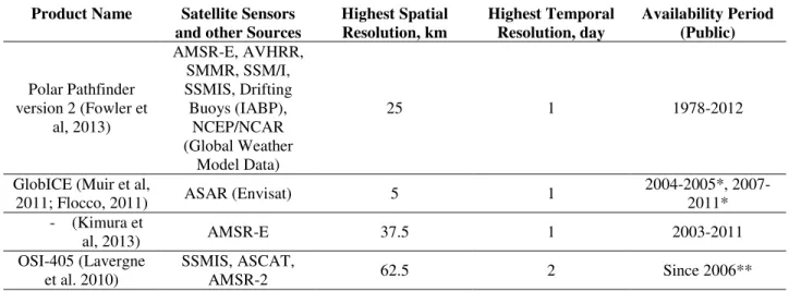
Several satellite-derived ice drift datasets are available online. These datasets differ from each other in spatial and temporal resolution, regional availability, availability period, source data and satellite sensor(s), techniques to infer ice motion from raw satellite data, and whether the dataset is gridded (Eulerian) or provides information about motion path of specific ice
features (Lagrangian). Some of the gridded datasets with data for the Beaufort Sea are introduced in Table 1.
Table 1 Some gridded ice drift datasets with data for the Beaufort Sea region
Product Name Satellite Sensors and other Sources
Highest Spatial Resolution, km Highest Temporal Resolution, day Availability Period (Public) Polar Pathfinder version 2 (Fowler et al, 2013) AMSR-E, AVHRR, SMMR, SSM/I, SSMIS, Drifting Buoys (IABP), NCEP/NCAR (Global Weather Model Data) 25 1 1978-2012
GlobICE (Muir et al,
2011; Flocco, 2011) ASAR (Envisat) 5 1
2004-2005*, 2007-2011* - (Kimura et al, 2013) AMSR-E 37.5 1 2003-2011 OSI-405 (Lavergne et al. 2010) SSMIS, ASCAT, AMSR-2 62.5 2 Since 2006**
* Only available for some months in fall, winter, spring period
** Data exists since 2002 but archived data on internet for public use is since 2006
Since the main focus of the present paper is the study of in-ice oil spill trajectory based on long term historical data, we selected the Polar Pathfinder version 2 dataset (Fowler et al, 2013), referred to as Polar Pathfinder from here on. The Polar Pathfinder dataset provides thirty-four years (1978-2012) of daily ice motion vectors with a 25 km spatial resolution. To prepare the Polar Pathfinder dataset, each source data, listed in Table 1, is “weighted” based on the
accuracy of the source data; the highest weight is given to observed drifting buoy data, if this data exists nearby. Spatial and temporal error estimates are also provided in the Polar Pathfinder dataset. Error estimates were not taken into account for most results given in the present paper. We have, however, included a separate section in the paper in which the effect of errors, given in the Polar Pathfinder dataset, in trajectories is studied by a Monte-Carlo approach.
(Sumata et al., 2014) has compared different satellite-derived ice drifts datasets, including the Polar Pathfinder, with each other and also with the observed buoy tracks collected through the International Arctic Buoy Programme (IABP); it is concluded that the difference between satellite-derived ice drifts and IABP observations is smaller when the ice concentration is high and/or when the ice thickness is large. The present study focuses on spills during the fall and winter seasons when generally ice is thick and highly concentrated.
3 Modelling and Analysis of In-ice Oil Spill Trajectories 3.1 Modelling Trajectories
Spill of oil is modelled by the “injection” of point “droplets” at the spill location at a constant frequency. For the present study, this constant frequency is daily which corresponds to the temporal resolution of the Polar Pathfinder data. Each droplet is, afterwards moved for a physical day based on the ice drift vector field spatially interpolated to the location of the
droplet. The spatial interpolation is linear and based on the three ice drift vectors at each node of the triangular Polar Pathfinder dataset grid cell in which the droplet is located. When, and if, the droplet leaves a cell during the movement, the spatial interpolation is then carried out with the three ice drift vectors of the new cell. No temporal interpolation is considered for the present study, i.e., ice drift data at each node is updated daily, temporal frequency of the drift dataset is 1 day, during the modelling period. The “injection” continues throughout the modelled spill
duration. All of the droplets are moved and tracked during the model duration. If a point, representing an oil droplet, reaches a cell whose any of the three nodes is associated with no valid ice drift data, e.g. open water, the droplet is stopped at that location; among all modelled scenarios, introduced later in the paper, the peak proportion of trajectories which are stopped, because of the above reason, in a scenario is approximately 4%.
As mentioned earlier, in the preparation of the Polar Pathfinder dataset, a higher weight was given to observed buoy data among the entire source data, see Table 1. This means that the Polar Pathfinder dataset probably involves less error close to observed IABP buoys. To verify the present trajectory modelling, we have then modelled the trajectory of a droplet released at the location of an IABP buoy (namely Buoy90008) and compared the observed and the modelled trajectories of the 1 November 2008 to 31 March 2009 period. Figure 1 shows this comparison. The difference between the observed and modelled trajectories could stem from different sources: (1) Polar Pathfinder has uncertainties, (2) ice drift changes over spatial scales of less than 25 km, Polar Pathfinder’s spatial resolution, cannot be resolved, (3) ice drift changes over temporal scales of less than 1 day, Polar Pathfinder’s temporal resolution, cannot be resolved.
Considering all the possible sources of error mentioned above, the overall shape of the modelled trajectory very closely resembles that of the observed buoy. The approximate
Figure 1 Reasonable accuracy of the present trajectory modelling when compared with an observed IABP buoy track. The distance between the start and the end locations is approximately 950 km.
3.2 Analyzing Trajectories
The total number of trajectories is equal to the number of injected droplets. All droplets that make a trajectory are considered for the analysis of the results. This means that all
intermediate droplets and the final locations of droplets are considered for the analysis; intermediate droplets are the locations of droplets before they reach their final locations at the end of model duration. All analyses are based on all trajectories. All analyses are based on an analysis grid, different from the Polar Pathfinder grid, composed of square grid cells covering the Beaufort Sea. If the dimension of the grid cell is very small, many cells will not contain any droplet which leads to spotty results including contamination probability as a function of location. If the dimension of the grid cell is very large, however, the results will not capture regions with high spatial gradients. After some tests, 5 km was found to be an optimum grid cell size. Note that findings of the present research, given later in section 5, do not depend on the size of the grid cell; the grid cell size is only adjusted to better visualize results. Unless noted
otherwise, all results are based on thirty-four years of historical Polar Pathfinder ice drifts. The following lists and explains the analysis of trajectories.
Contamination Probability: This is the probability that oil reaches a location. To calculate the
probability, the total number of years when a cell contained a droplet are counted and divided by the total number of modelled years, 34 years. A year is not counted more than once if a cell has more than one droplet in it in that year. For example if a cell “sees” droplets in 5 different years out of the total 34 years, the contamination probability for the cell is 5/34.
Contamination Intensity: This is a measure of how frequently a location is contaminated. To
calculate the intensity, the total number of droplets in a cell are counted and divided by the total number of droplets. For example if a cell contains 2000 droplets out of total of 50000 droplets, the contamination intensity is 2/50.
Contamination Probability of Territorial Water Boundary: Territorial waters of a country
are usually defined as regions whose seaward boundary extends up to 12 nautical miles, Start Location, 1 Nov. 2008 Final Locations, 31 March 2009
approximately 22.24 km, from the country’s coastlines. In the present study we calculated the chance that the length of the seaward contaminated territorial water boundary exceeds different values (exceedance probability). The territorial water boundary in the present study is defined as being 25 km offshore of the shoreline. This boundary is shown as a dashed black line in the rest of the figures. Polar Pathfinder dataset involves high level of uncertainty on nodes immediately offshore; considering that the spatial resolution of the triangular dataset grid is 25 km, we have selected the territorial boundary over the actual shoreline to avoid the high uncertainty nodes. To calculate the exceedance probability, the boundary is intersected with results of contamination probabilities explained above. Values of contamination probability of cells that contain any portion of the boundary are then considered to calculate the exceedance values.
Both the deterministic and the probabilistic trajectory modelling were simulated using the National Research Council of Canada’s proprietary EnSim™ computer software framework. Analysis and visualization of results were carried out using the open source freeware R and python. Raw Polar Pathfinder dataset is publically available online. The processed ready-to-use dataset, which is input to the model, was obtained from the National Research Council of Canada’s proprietary Beaufort Sea Engineering Database. Note that the developed tools for the modelling and analysis of in-ice spills are not limited to the shape of the ice drift grid cells, nor are they limited to the ice drift dataset’s spatial and temporal resolutions.
4 In-ice Oil Spill Scenarios
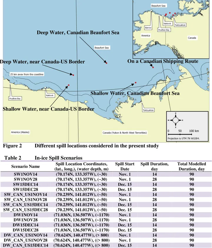
Several in-ice oil spill scenarios were considered. The scenarios are defined by the spill location, duration, start date, and the total modelled duration. Scenarios include deep and shallow water spills in the Canadian Beaufort. Other scenarios include near the Canada-US border deep and shallow water spills and tanker spills on a Canadian shipping route. Most scenarios involve 2 and 4 week spill durations and ninety days of total modelled duration. For the tanker spills, the spill, and total modelled durations are 3, and 30 days, respectively. Table 2 provides the details of the modelled scenarios and Figure 2 shows different spill locations considered in the present study.
Figure 2 Different spill locations considered in the present study
Table 2 In-ice Spill Scenarios
Scenario Name Spill Location Coordinates, (lat., long.), (water depth, m)
Spill Start Date Spill Duration, day Total Modelled Duration, day SW1NOV14 (70.174N, 133.357W), (~30) Nov. 1 14 90 SW1NOV28 (70.174N, 133.357W), (~30) Nov. 1 28 90 SW15DEC14 (70.174N, 133.357W), (~30) Dec. 15 14 90 SW15DEC28 (70.174N, 133.357W), (~30) Dec. 15 28 90 SW_CAN_US1NOV14 (70.239N, 141.012W), (~50) Nov. 1 14 90 SW_CAN_US1NOV28 (70.239N, 141.012W), (~50) Nov. 1 28 90 SW_CAN_US15DEC14 (70.239N, 141.012W), (~50) Dec. 15 14 90 SW_CAN_US15DEC28 (70.239N, 141.012W), (~50) Dec. 15 28 90 DW1NOV14 (71.036N, 136.507W), (~1170) Nov. 1 14 90 DW1NOV28 (71.036N, 136.507W), (~1170) Nov. 1 28 90 DW15DEC14 (71.036N, 136.507W), (~1170) Dec. 15 14 90 DW15DEC28 (71.036N, 136.507W), (~1170) Dec. 15 28 90 DW_CAN_US1NOV14 (70.624N, 140.477W), (> 800) Nov. 1 14 90 DW_CAN_US1NOV28 (70.624N, 140.477W), ((> 800) Nov. 1 28 90 DW_CAN_US15DEC14 (70.624N, 140.477W), ((> 800) Dec. 15 14 90 DW_CAN_US15DEC28 (70.624N, 140.477W), ((> 800) Dec. 15 28 90 CSR1NOV3 (70.66N, 131.121W), (~45) Nov. 1 3 30 CSR15DEC3 (70.66N, 131.121W), (~45) Dec. 15 3 30
Shallow Water, near Canada-US Border Deep Water, near Canada-US Border
Deep Water, Canadian Beaufort Sea
Shallow Water, Canadian Beaufort Sea
5 Findings of Modelled In-ice Spill Scenarios
This section summarizes the major findings based on the analysis of the results of the modelled scenarios. The appendix includes all result figures for scenarios involving a twenty eight-day long spill duration and the two scenarios involving spills on a Canadian Shipping route.
Regardless of spill scenario, the dominant direction of spill extent is towards the west. This is consistent with the well-known clockwise surface currents direction in the Beaufort Sea known as the Beaufort Gyre.
Note that the following results are based on the above eighteen scenarios and not based on a detailed parametric study.
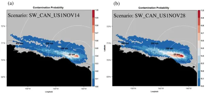
Spill Extent as a Function of Spill Start Date
The extent of spills is generally larger when the start date of the spill is Nov. 1st than when it is Dec. 15th. This is particularly true when the extent of the spill is considered as the outer edge of regions with contamination probability of 10% and above. This larger extent is generally along both the east-west and north-south directions, Figure 3. This larger extent of the spill is associated with a generally larger intensity as defined in the previous section.
Figure 3 The extent of the spill is generally larger when the spill starts on 1 Nov. (a), than when it starts on 15 Dec. (b). The dashed black line is 25 km away from the coastline. White circles are centered at spill locations and the distances on circles are radii.
Spill Extent as a Function of Spill Location
The extent of spills tends to be larger when the spill is in deep waters than when it is in shallow waters, Figure 4. This is particularly true when the extent of the spill is considered as the outer edge of regions with contamination probability of 10% and above. The extent of the spill is similar between the two deep water spill scenario series, deep water in the Canadian Beaufort and deep waters close to Canada-US border. The extent of the spill is similar between the two shallow water spill scenario series, shallow water in the Canadian Beaufort and shallow water close to Canada-US border.
(a)
Scenario: DW1NOV28
(b)
Figure 4 Scenario results suggest that deep water spills, (a), extend more than shallow water spills, (b).
Spill Extent as a Function of Spill Duration
The effect of spill duration on the extent of the spill is as expected: the longer duration is associated with the extension of the higher contamination probability regions. The extent of regions with smaller contamination probability values is generally unchanged when the spill duration is increased from two weeks to four weeks, Figure 5.
Figure 5 For longer lasting spills, the high contamination probability regions extend more than low contamination probability regions. (a) A 2-week long spill, (b) A 4-week long Spill. Note that the total modelled duration in both figures is 90 days.
The contamination intensity, as defined in sub-section 3.2., does not necessarily drop with distance from the spill location; this is seen in one of the modelled scenarios and shown in Figure 6. Perhaps, depending on the location of the spill, its duration, and the shape of the coastline, there could be regions where the contamination intensities are of comparable values to those of the spill location. For the specific scenario associated with Figure 6, clean-up efforts
(b) Scenario: SW1NOV14 (a) Scenario: DW_CAN_US1NOV14 (a) Scenario: SW_CAN_US1NOV14 (b) Scenario: SW_CAN_US1NOV28
could be perhaps both focused at the spill location and the other high contamination intensity location close to the coastline.
Figure 6 The contamination intensity is not only high at the location of the spill; it could be also high in other locations perhaps depending on the spill location and duration and the shape of the coastline.
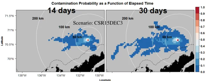
Spill Extent as a Function of Elapsed Time
The speed of oil slick motion is not a significant function of elapsed time during the total modelled duration, which is mainly 90 days except for the modelled tanker spill scenarios for which the total modelled duration is 30 days, Figure 7. The spill appears to move steadily with time. See the Appendix for similar results for some other scenarios.
Figure 7 The speed of the spread of spills is not a strong function of elapsed time. Each figure above is a snapshot of contamination probability at different elapsed times. Affected Territorial Waters Boundary
The chance of coastline contamination is expected to be higher when a spill occurs in shallow waters than when the spill occurs in deep waters. This is because shallow waters are usually closer to coastlines than deep waters. This expectation is confirmed by visualizing the exceedance probability of contamination of the territorial water boundary for modelled scenarios. Figure 8 shows this probability for scenarios involving spills in shallow waters of the Canadian Beaufort and at a shallow-water location close to the Canada-US border. Figure 8 shows that the maximum possible length of contamination is higher for the border spill (< 500 km), Figure 8a than it is for the other case (< 350 km), Figure 8b. Earlier and longer-lasting spills are generally associated with larger contamination length. The appendix provides similar figures for all the other scenarios.
Figure 8 Shallow water, earlier, and longer-lasting spills are generally associated with longer contaminated territorial water boundaries. The exceedance probability of
contamination of the territorial water boundary for shallow water spills: (a) close to Canada-US border, (b) the Canadian Beaufort. Note that extents of the horizontal axes in the above figures are different.
6 Effects of Polar Pathfinder Dataset Uncertainty on Modelled Trajectories
Error estimates, root-mean-square of error, of the Polar Pathfinder ice drift calculations have been provided in the source dataset. In this section we briefly study how the inclusion of
Scenario: CSR15DEC3
(a)
Polar Pathfinder errors changes the modelled trajectories.
The Polar Pathfinder error estimates are a function of time and location. The mean value of error, however, has only been reported for the whole dataset’s spatial and temporal extent; it is reported (Miller et al. 2006) that the mean error in the east-west and the north-south components of the Polar Pathfinder ice velocity vector are respectively 0.1 cm/s, and 0.4 cm/s.
To model uncertainty, we perturb the raw ice drift data by the spatially and temporally varying errors. This perturbation assumes a normal distribution of error with the mean values given above. So a point, representing an oil droplet, is moved based on perturbed ice velocity vectors as the point passes through the computational domain from one Polar Pathfinder dataset grid cell to another. With this approach, it is almost certain to have a different velocity field at the same location in space-time coordinate when the trajectory model is re-run. We then model the same scenario many times, a Monte-Carlo approach, to gain an understanding about how uncertainties affect the fate of the in-ice spills.
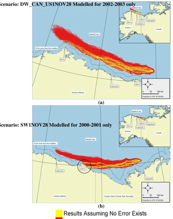
Two scenarios, DW_CAN_US1NOV28, and SW1NOV28, see Table 2, were selected for this uncertainty modelling. For each scenario, we identified the season associated with the largest spill extent and then modelled the uncertainty for that season. The season for the first scenario is 2002-2003 and for the second scenario, it is 2000-2001. Figure 9 compares the trajectories based on the raw, assuming no error, Polar Pathfinder data and Monte-Carlo modelling. We compared the Monte-Carlo results based on one hundred and five hundred runs; the extent of the two modelled spills, particularly the east-west extent of the spill, was only slightly different. Monte-Carlo results given in Figure 9 are based on one hundred runs.
Uncertainties lead to the expansion of the contaminated region. This expansion tends to be more seaward than towards the coastline. This is because the mean error and the standard deviation of the error for the north-south component of ice velocity vectors are in a way that this vector component usually gains a positive value towards the sea. As a result, the inclusion of uncertainties does not lead to trajectories which are closer the coastline than they are for the case when no error is considered.
Along the coastline direction, two different behaviors are seen. When the raw data trajectories “hit” the coastline, there is a chance that when errors are included, the trajectories “miss” the coastline. When this happens, the trajectories could move a relatively large distance beyond the coastline location where raw data trajectories are settled, see the black circle in Figure 9b. Note that the Polar Pathfinder ice drift dataset is generally less accurate for locations very close to the coastline compared with other locations. The other behavior happens when the raw data trajectories do not “hit” the coastline in which case the extension of the trajectories, when errors are included, are not significantly different from the extent, along the coastline, of raw data trajectories.
(a)
(b)
Figure 9 Trajectories based on raw Data, assuming no error exists, and Monte-Carlo uncertainty modelling approach. Including uncertainties do not generally lead to closer to coastline trajectories and depending on whether raw data trajectories "hit" the coastline, the along the coastline extent of the Monte-Carlo trajectories change. (a) A deep water spill near the Canada-US border for 2002-2003 season, (b) A shallow water Canadian Beaufort spill for 2000-2001 season.
Scenario: DW_CAN_US1NOV28 Modelled for 2002-2003 only
7 Concluding Remarks
Several hypothetical scenarios of in-ice oil spill in the Beaufort Sea were modelled and studied. The start and the temporal extent of the modelled scenarios are within the fall and winter period during which the concentration of ice is very high. It was assumed that in this period, the spilled oil only moves with sea ice. The motion of ice is based on a satellite-derived dataset named Polar Pathfinder version 2.
A model was developed to calculate the spill trajectories of in-ice oil based on the ice motion dataset in both deterministic, assuming no error is involved, and probabilistic modes. The observed trajectory of a buoy was compared with the modelled trajectory; the two trajectories were very similar. An additional tool was developed to analyze and visualize trajectory results which were based on thirty four years of ice motion vectors.
Contamination probability and intensity and also the time dependence of the spread of spills were studied. Some of the findings are:
• The extent of the spill is generally larger when the spill starts on 1 Nov. than when it starts on 15 Dec.
• Scenario results suggest that deep water spills move away from spill location more than they do for shallow water spills.
• For longer-lasting spills, high contamination probability regions extend more than the low contamination probability regions.
• The contamination intensity is not only high at the location of the spill; it could be also high in other locations perhaps depending on the spill location and duration and the shape of the coastline.
• The speed of the spread of spills is not a strong function of elapsed time.
• Shallow water, earlier, and longer-lasting spills are generally associated with longer contaminated territorial water boundaries.
Results uncertainties were also modelled by the developed tool’s probabilistic modelling capability through a Monte-Carlo approach. Trajectories with and without errors in the input ice drift dataset were studied and compared.
Future efforts will be focused on (1) the comparison of the present in-ice oil spill trajectory approach with other model results, (2) a detailed parametric approach to study the effect of different parameters on trajectory of spills, and (3) a more in-depth study of the effects of uncertainties in the spread of in-ice oil spills.
8 Acknowledgments
The authors thank the Arctic Program of the National Research Council of Canada for the financial support of the study. The authors thank Philippe Lamontagne from the National
Research Council of Canada for his help with the processing and formatting of the latest version of the Polar Pathfinder Dataset, and Ron Saper formerly with the National Research Council of Canada and Ronald Kwok from the Jet Propulsion Laboratory, California Institute of
Technology, for their guidance for the uncertainty modelling section of the present research.
Bailey, A., “USGS: 25% Arctic Oil, Gas Estimate a Reporter’s Mistake”, Petroleum News, 12, 42, 2007.
Blanken, H., B. Tremblay, S. Gaskin, and A. Slavin, “A Numerical Risk Assessment for Spills from Oil and Gas Activity around the Arctic Ocean Basin”, in E-Proceedings of the Thirty-six
IAHR World Congress, The Hague, The Netherlands, 4 p., 2015.
Chen, E.C., “Arctic Winter Oil Spill Test”, Environment Canada Technical Bulletin, 68, 20 p., 1972.
Drozdowski, A., S. Nudds, C.G. Hannah, H. Niu, I.K. Peterson, and W.A. Perrie, “Review of Oil Spill Trajectory Modelling in the Presence of Ice”, Canadian Technical Report of
Hydrography and Ocean Sciences 274, Fisheries and Oceans Canada, 92 p., 2011.
Eurasia Group, “Opportunities and Challenges for Arctic Oil and Gas Development”, The Wilson Center, Washington, D.C., 29 p., 2014.
Fingas, M.F. and B.P. Hollebone, “Review of Behaviour of Oil in Freezing Environments”,
Marine Pollution Bulletin, 47:333-340, 2003.
Flocco, D., “GlobICE Product Validation Report”, University College London, GI-RP-VAR-4003, 38 p., 2011.
Fowler, C., J. Maslanik, W. Emery, and M. Tschudi, (2013),Polar Pathfinder Daily 25 km EASE-Grid Sea Ice Motion Vectors, Version 2. Retrieved November, 2015 from
dx.doi.org/10.5067/LHAKY495NL2T.
Gearon, M.S., D.F. McCay, E. Chaite, S. Zamorski, D. Reich, J. Rowe, and D. Schmidt-Etkin, “SIMAP Modelling of Hypothetical Oil Spills in the Beaufort Sea for World Wildlife Fund (WWF)”, Applied Science Associates, P13-235, 311 p., 2014.
Kimura, N. , A. Nishimura, Y. Tanaka, and H. Yamaguchi, “Influence of Winter Sea Ice Motion on Summer Ice Cover in the Arctic”, Polar Research, 32, 20193, 2013.
Lavergne, T., S. Eastwood, Z. Teffah, H. Schyberg, and L.-A.Breivik, “Sea Ice Motion from Low Resolution Satellite Sensors: An Alternative Method and its Validation in the Arctic”,
Journal of Geophysical Research, Oceans, 115, C10032, 2010.
LOOKNorth, “Oil Spill Detection and Modeling in the Hudson and Davis Straits”, Nunavut Planning Commission, R-13-087-1096, 274 p., 2014.
Miller, P.A., S.W. Laxon, D.L. Feltham, and D.J. Cresswell, “Optimization of a Sea Ice Model Using Basinwide Observations of Arctic Sea Ice Thickness, Extent, and Velocity”, Journal of
Mouawad, J., (2008), Oil Survey Says Arctic Has Riches. Retrieved March, 2016 from nytimes.com/2008/07/24/business/24arctic.html?_r=0
Muir, A., S. Baker, S.W. Laxon, J. Ridley, and R. Kwok, “Arctic Sea Ice Dynamics for Climate Models: GlobICE Project Results and Products”, American Geophysical Union, abstract #C52B-04, 2011.
Nudds, S.H., A. Drozdowski, Y. Lu, and S. Prinsenberg, “Simulating Oil Spill Evolution in Water and Sea Ice in the Beaufort Sea”, in Proceedings of the Twenty-third International
Offshore and Polar Engineering, Anchorage, USA, pp. 1066-1071, 2013.
Sumata, H., T. Lavergne, F. Girard-Ardhuin, N. Kimura, M.A. Tschudi, F. Kauker, M. Karcher, and R. Gerdes, “An Intercomparison of Arctic Ice Drift Products to Deduce Uncertainty
Estimates”, Journal of Geophysical Research, Oceans, 119, 8, 2014.
10 Appendix
Remaining results of scenarios related to the Canadian shipping route and all other scenarios involving twenty eight-day long spills and exceedance probability plots for the contaminated territorial water boundary for all scenarios.
CSR1NOV3
DW_CAN_US1NOV28
DW1NOV28
SW_CAN_US1NOV28
SW1NOV28