ECCO Version 4: Second Release
G. Forget
1
, J.-M. Campin
1
, P. Heimbach
1
,
2
,
3
, C. N. Hill
1
, R.
M. Ponte
4
, and C. Wunsch
5
1Dept. of Earth, Atmospheric and Planetary Sciences, Massachusetts Institute of Technology, Cambridge
MA 02139 USA;2Institute for Computational Engineering and Sciences, The University of Texas at Austin,
Austin, TX 78712, USA;3Jackson School of Geosciences, The University of Texas at Austin, Austin, TX
78712, USA;4Atmospheric and Environmental Research, Inc., Lexington MA 02421 USA;5Dept. of Earth and Planetary Sciences, Harvard University, Cambridge, MA 02139 USA
The purpose of this note is twofold: (1) document the second release of ECCO version 4 state estimates (ECCO v4-r2); (2) provide a citable identifier to distinguish it from the previous release (ECCO v4-r1; Forget et al 2015).
Access ECCO v4-r2:online access is free and unrestricted via http://ecco-group.org/ ; at the time of writing the ECCO v4-r2 files are accessed via ftp://mit.ecco-group.org/ecco_for_las/version_4/release2/ and http://mit.ecco-group.org/opendap/ecco_for_las/version_4/release2/contents.html
Software Used for ECCO v4-r2:the state estimate output files (provided online) and its depiction (provided below) were produced using the ‘checkpoint64u’ versions of the general circulation model (MITgcm and ECCO v4 settings) and Matlab analysis toolboxes (gcmfaces and MITprof).
Solution History:the 1992-2011 solution documented here (ECCO v4-r2) is a minor update to the original ECCO v4 solution documented by Forget et al 2015 (ECCO v4-r1). As compared with ECCO v4-r1 (see Forget et al 2015 for details and notations) ECCO v4-r2 benefits from a few additional corrections in the model settings:
1. Inclusion of geothermal heating at the sea floor in MITgcm and ECCO v4 settings.
2. Inclusion of Kgmand Kσinterpolation to C-grid velocity points in MITgcm and ECCO v4 settings. 3. Re-inclusion of targeted bottom viscosity in ECCO v4 settings.
4. Re-inclusion of estimated wind stress adjustments over 2000-2011 in ECCO v4 settings.
5. Re-adjustment of ECCO v4 global mean precipitation (homogeneously) to match the AVISO global mean sea level time series (http://www.aviso.altimetry.fr/).
Contents Included Below:the gcmfaces ‘standard analysis’ (introduced in Forget et al. 2015) appended below for ECCO v4-r2 depicts routinely monitored characteristics of ECCO solutions. It allows for direct comparison with the published ECCO v4-r1 standard analysis (doi:10.5194/gmd-8-3071-2015-supplement).
References:Forget, G., J.-M. Campin, P. Heimbach, C. N. Hill, R. M. Ponte, and C. Wunsch, 2015: ECCO version 4: an integrated framework for non-linear inverse modeling and global ocean state estimation. Geoscientific Model Development, 8, 3071-3104, doi:10.5194/gmd-8-3071-2015 (http://www.geosci-model-dev.net/8/3071/2015/)
Table of contents
fit to data fit to in situ data fit to altimeter data (RADS) fit to sst data
fit to seaice data volume, heat and salt transports
barotropic streamfunction meridional streamfunction
meridional streamfunction (time series) meridional heat transport
meridional freshwater transport meridional salt transport meridional transports (time series) transects transport
mean and variance maps
sea surface height 3D state variables air-sea heat flux air-sea freshwater flux surface wind stress global, zonal, regional averages
zonal mean tendencies equatorial sections global mean properties zonal mean properties zonal mean properties (surface) seaice time series
mixed layer depth fields
budgets : volume, heat and salt (top to bottom) budgets : volume, heat and salt (100m to bottom)
fit to in situ data
Figure :
Time mean misfit (model-data) for in situ profiles, at various
fit to in situ data
1995 2000 2005 2010 6000 5500 5000 4500 4000 3500 3000 2500 2000 1500 1000 800 600 400 200 0 depth (in m)mean cost for T: 1.71 (median: 0.536)
0 2 4 6 8 latitude normalized misfit pdf −50 0 50 −5 0 5 0 0.1 0.2 0.3 0.4 0.5 1995 2000 2005 2010 6000 5500 5000 4500 4000 3500 3000 2500 2000 1500 1000 800 600 400 200 0 depth (in m)
mean cost for S: 1.8 (median: 0.578)
0 2 4 6 8 latitude normalized misfit pdf −50 0 50 −5 0 5 0 0.1 0.2 0.3 0.4 0.5
Figure :
Cost function (top) for in situ profiles, as a function of depth
and time. Distribution of normalized misfits (bottom) as a function of
latitude. For T (left) and S (right).
fit to in situ data
normalized misfit atlExt_25N90N_misDisT 2000 2010 −5 0 5 0 0.1 0.2 0.3 0.4 pacExt_25N90N_misDisT 2000 2010 −5 0 5 0 0.1 0.2 0.3 0.4 arct_25N90N_misDisT 2000 2010 −5 0 5 0 0.1 0.2 0.3 0.4 normalized misfit atlExt_25S25N_misDisT 2000 2010 −5 0 5 0 0.1 0.2 0.3 0.4 pacExt_25S25N_misDisT 2000 2010 −5 0 5 0 0.1 0.2 0.3 0.4 indExt_25S25N_misDisT 2000 2010 −5 0 5 0 0.1 0.2 0.3 0.4 normalized misfit atlExt_90S25S_misDisT 2000 2010 −5 0 5 0 0.1 0.2 0.3 0.4 pacExt_90S25S_misDisT 2000 2010 −5 0 5 0 0.1 0.2 0.3 0.4 indExt_90S25S_misDisT 2000 2010 −5 0 5 0 0.1 0.2 0.3 0.4Figure :
Distribution of normalized misfits per basin (panel) as a function
fit to in situ data
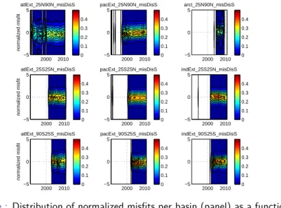
normalized misfit atlExt_25N90N_misDisS 2000 2010 −5 0 5 0 0.1 0.2 0.3 0.4 pacExt_25N90N_misDisS 2000 2010 −5 0 5 0 0.1 0.2 0.3 0.4 arct_25N90N_misDisS 2000 2010 −5 0 5 0 0.1 0.2 0.3 0.4 normalized misfit atlExt_25S25N_misDisS 2000 2010 −5 0 5 0 0.1 0.2 0.3 0.4 pacExt_25S25N_misDisS 2000 2010 −5 0 5 0 0.1 0.2 0.3 0.4 indExt_25S25N_misDisS 2000 2010 −5 0 5 0 0.1 0.2 0.3 0.4 normalized misfit atlExt_90S25S_misDisS 2000 2010 −5 0 5 0 0.1 0.2 0.3 0.4 pacExt_90S25S_misDisS 2000 2010 −5 0 5 0 0.1 0.2 0.3 0.4 indExt_90S25S_misDisS 2000 2010 −5 0 5 0 0.1 0.2 0.3 0.4Figure :
Distribution of normalized misfits per basin (panel) as a function
fit to altimeter data (RADS)
fit to altimeter data (RADS)
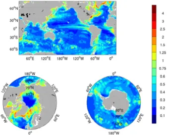
Figure :
log(prior error variance) – sea level anomaly (m
2
) – large
fit to altimeter data (RADS)
fit to altimeter data (RADS)
fit to altimeter data (RADS)
Figure :
modeled-observed log(variance) – sea level anomaly (m
2
) – large
fit to altimeter data (RADS)
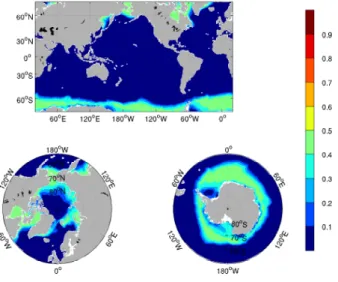
Figure :
modeled-observed log(variance) – sea level anomaly (m
2
) –
fit to altimeter data (RADS)
fit to altimeter data (RADS)
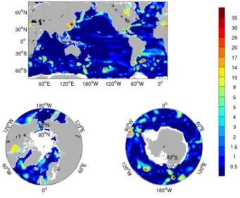
Figure :
modeled-observed cost – sea level anomaly
fit to altimeter data (RADS)
fit to altimeter data (RADS)
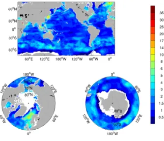
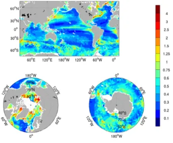
Figure :
observed log(variance) – sea level anomaly (m
2
) – large
fit to altimeter data (RADS)
fit to altimeter data (RADS)
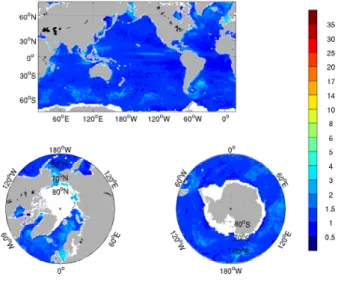
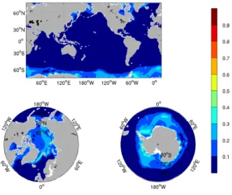
Figure :
modeled log(variance) – sea level anomaly (m
2
) – large
fit to altimeter data (RADS)
fit to sst data
fit to sst data
fit to sst data
fit to sst data
fit to seaice data
fit to seaice data
fit to seaice data
fit to seaice data
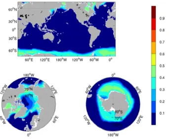
Figure :
ECCO (left) and NSIDC (right, gsfc bootstrap) ice
fit to seaice data
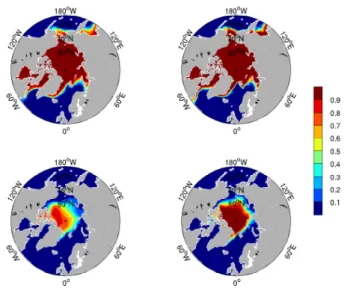
Figure :
ECCO (left) and NSIDC (right, gsfc bootstrap) ice
fit to seaice data
1995 2000 2005 2010 0 0.2 0.4 0.6 0.8 1 1.2 1.4 1.6 1.8 2x 10 13 m 2 Northern Hemisphere 1995 2000 2005 2010 0 0.2 0.4 0.6 0.8 1 1.2 1.4 1.6 1.8 2x 10 13 m 2 Southern HemisphereFigure :
ECCO (blue) and NSIDC (red, gsfc bootstrap) ice concentration
in March and September in Northern Hemisphere (left) and Southern
Hemisphere (right)
fit to seaice data
1995 2000 2005 2010 0 1 2 3 4 5x 10 12 m 2Entire Southern Ocean
1995 2000 2005 2010 0 1 2 3 4x 10 11 m 2 20E to 90E 1995 2000 2005 2010 0 2 4 6x 10 11 m 2 90E to 160E 1995 2000 2005 2010 0 5 10 15x 10 11 m 2 160E to −130E 1995 2000 2005 2010 0 2 4 6x 10 11 m 2 −130E to −62E 1995 2000 2005 2010 0 0.5 1 1.5 2x 10 12 m 2 −62E to 20E
Figure :
ECCO (blue) and NSIDC (red, gsfc bootstrap) ice concentration
fit to seaice data
1995 2000 2005 2010 1.5 1.55 1.6 1.65 1.7x 10 13 m 2Entire Southern Ocean
1995 2000 2005 2010 2.5 3 3.5 4x 10 12 m 2 20E to 90E 1995 2000 2005 2010 1.2 1.4 1.6 1.8 2x 10 12 m 2 90E to 160E 1995 2000 2005 2010 3 3.5 4 4.5x 10 12 m 2 160E to −130E 1995 2000 2005 2010 1 1.5 2 2.5x 10 12 m 2 −130E to −62E 1995 2000 2005 2010 5 5.5 6 6.5 7x 10 12 m 2 −62E to 20E
Figure :
ECCO (blue) and NSIDC (red, gsfc bootstrap) ice concentration
barotropic streamfunction
barotropic streamfunction
meridional streamfunction
meridional streamfunction
meridional streamfunction
meridional streamfunction
meridional streamfunction
meridional streamfunction
Figure :
1992-2011 standard deviation – Atlantic overturning
meridional streamfunction (time series)
19920 1994 1996 1998 2000 2002 2004 2006 2008 2010 2012 2 4 6 8 10 12 14 16 18 20annual global overturning at ≈ 1000m depth (Sv)
25N 35N 45N 55N
meridional streamfunction (time series)
19920 1994 1996 1998 2000 2002 2004 2006 2008 2010 2012 2 4 6 8 10 12 14 16 18 20annual atlantic overturning at ≈ 1000m depth
25N 35N 45N 55N
Figure :
annual Atlantic overturning at select latitudes at ≈ 1000m depth
meridional heat transport
−80
−60
−40
−20
0
20
40
60
80
−2
−1.5
−1
−0.5
0
0.5
1
1.5
2
Meridional Heat Transport (in PW)
global
Atlantic
Pacific+Indian
meridional heat transport
−80
−60
−40
−20
0
20
40
60
80
0
0.5
1
1.5
2
2.5
3
3.5
4
Meridional Heat Transport (in PW)
global
Atlantic
Pacific+Indian
meridional freshwater transport
−80
−60
−40
−20
0
20
40
60
80
−1.5
−1
−0.5
0
0.5
1
1.5
2
Meridional Freshwater Transport (in Sv)
global
Atlantic
Pacific+Indian
meridional freshwater transport
−80
−60
−40
−20
0
20
40
60
80
0
0.2
0.4
0.6
0.8
1
1.2
1.4
1.6
1.8
2
Meridional Freshwater Transport (in Sv)
global
Atlantic
Pacific+Indian
Figure :
1992-2011 standard deviation – meridional freshwater transport
meridional salt transport
−80
−60
−40
−20
0
20
40
60
80
−50
−40
−30
−20
−10
0
10
20
30
40
50
Meridional Salt Transport (in psu.Sv)
global
Atlantic
Pacific+Indian
meridional salt transport
−80
−60
−40
−20
0
20
40
60
80
0
10
20
30
40
50
60
Meridional Salt Transport (in psu.Sv)
global
Atlantic
Pacific+Indian
Figure :
1992-2011 standard deviation – meridional salt transport
meridional transports (time series)
meridional transports (time series)
meridional transports (time series)
transects transport
1995
2000
2005
2010
−1
0
1
2
3
Bering Strait (>0 to Arctic) (mean = 1.04 Sv)
1995
2000
2005
2010
−3
−2
−1
0
1
Davis Strait (>0 to Arctic) (mean = −1.5 Sv)
1995
2000
2005
2010
−6
−4
−2
Denmark Strait (>0 to Arctic) (mean = −5.95 Sv)
1995
2000
2005
2010
0
2
4
6
8
Iceland Faroe (>0 to Arctic) (mean = 4.54 Sv)
1995
2000
2005
2010
−4
−2
0
2
4
Faroe Scotland (>0 to Arctic) (mean = 1.72 Sv)
1995
2000
2005
2010
−0.5
0
0.5
Scotland Norway (>0 to Arctic) (mean = 0.05 Sv)
transects transport
1995
2000
2005
2010
20
25
30
35
40
Florida Strait (>0 to Atlantic)
(mean = 29.89 Sv)
1995
2000
2005
2010
20
25
30
35
40
Florida Strait W1 (>0 to Atlantic)
(mean = 28.57 Sv)
1995
2000
2005
2010
−1
0
1
2
3
Florida Strait E1 (>0 to Atlantic)
(mean = 2.43 Sv)
1995
2000
2005
2010
−6
−4
−2
0
2
Florida Strait E2 (>0 to Atlantic)
(mean = −3.75 Sv)
transects transport
1994
1996
1998
2000
2002
2004
2006
2008
2010
0.4
0.5
0.6
0.7
0.8
0.9
1
1.1
Gibraltar Overturn (upper ocean transport towards Med.)
(mean = 0.73 Sv)
transects transport
1995
2000
2005
2010
120
140
160
180
Drake Passage (>0 westward)
(mean = 155.12 Sv)
1995
2000
2005
2010
140
160
180
200
Madagascar Antarctica (>0 westward)
(mean = 180.01 Sv)
1995
2000
2005
2010
−40
−30
−20
−10
Madagascar Channel (>0 westward)
(mean = −23.86 Sv)
1995
2000
2005
2010
140
160
180
200
Australia Antarctica (>0 westward)
(mean = 171.35 Sv)
transects transport
1994
1996
1998
2000
2002
2004
2006
2008
2010
5
10
15
20
25
Indonesian Throughflow (>0 toward Indian Ocean)
(mean = 15.53 Sv)
sea surface height
sea surface height
sea surface height
Figure :
1992-2011 standard deviation – sea surface height (EXCLUDING
sea surface height
Figure :
1992-2011 standard deviation – sea surface height (INCLUDING
3D state variables
3D state variables
3D state variables
3D state variables
3D state variables
3D state variables
3D state variables
3D state variables
3D state variables
3D state variables
3D state variables
3D state variables
3D state variables
3D state variables
3D state variables
3D state variables
3D state variables
3D state variables
3D state variables
3D state variables
3D state variables
3D state variables
3D state variables
3D state variables
3D state variables
3D state variables
Figure :
1992-2011 standard deviation – vertical velocity (in mm/year) at
3D state variables
3D state variables
Figure :
1992-2011 standard deviation – vertical velocity (in mm/year) at
3D state variables
3D state variables
Figure :
1992-2011 standard deviation – vertical velocity (in mm/year) at
3D state variables
3D state variables
Figure :
1992-2011 standard deviation – vertical velocity (in mm/year) at
3D state variables
3D state variables
Figure :
1992-2011 standard deviation – vertical velocity (in mm/year) at
3D state variables
3D state variables
Figure :
1992-2011 standard deviation – vertical velocity (in mm/year) at
air-sea heat flux
air-sea heat flux
air-sea heat flux
air-sea heat flux
air-sea freshwater flux
air-sea freshwater flux
air-sea freshwater flux
air-sea freshwater flux
surface wind stress
surface wind stress
surface wind stress
surface wind stress
zonal mean tendencies
Figure :
1992-2011 , last year minus first year – zonal mean temperature
equatorial sections
Figure :
1992-2011 mean – equator temperature (degC;top) and zonal
global mean properties
1994 1996 1998 2000 2002 2004 2006 2008 2010 0 0.05 0.1 0.15 0.2Global Mean Sea level (m, uncorrected free surface)
monthly annual mean 1994 1996 1998 2000 2002 2004 2006 2008 2010 3.58 3.59 3.6
3.61 Global Mean Temperature (degC)
monthly annual mean 1994 1996 1998 2000 2002 2004 2006 2008 2010 34.724 34.725 34.726 34.727
Global Mean Salinity (psu)
monthly annual mean
global mean properties
Figure :
global mean temperature (K; top) and salinity (psu; bottom)
zonal mean properties
Figure :
mean temperature (top; K) and salinity (bottom; psu) minus
zonal mean properties
Figure :
mean temperature (top; K) and salinity (bottom; psu) minus
zonal mean properties
Figure :
mean temperature (top; K) and salinity (bottom; psu) minus
zonal mean properties
Figure :
mean temperature (top; K) and salinity (bottom; psu) minus
zonal mean properties
Figure :
mean temperature (top; K) and salinity (bottom; psu) minus
zonal mean properties
Figure :
mean temperature (top; K) and salinity (bottom; psu) minus
zonal mean properties
Figure :
mean temperature (top; K) and salinity (bottom; psu) minus
zonal mean properties
Figure :
mean temperature (top; K) and salinity (bottom; psu) minus
zonal mean properties
Figure :
mean temperature (top; K) and salinity (bottom; psu) minus
zonal mean properties (surface)
Figure :
zonal mean temperature (degC; top) and salinity (psu; bottom)
zonal mean properties (surface)
Figure :
zonal mean SSH (m, uncorrected free surface) minus first year,
zonal mean properties (surface)
Figure :
zonal mean ice concentration (no units) and mixed layer depth
seaice time series
1994 1996 1998 2000 2002 2004 2006 2008 2010 0 5 10 15 20Northern Hemisphere ice cover (in 1012m2)
monthly annual mean 1994 1996 1998 2000 2002 2004 2006 2008 2010 0 5 10 15 20 25
Southern Hemisphere ice cover (in 1012m2)
monthly annual mean
Figure :
sea ice cover (in 10
12
m
2
) in northern (top) and southern
seaice time series
1994 1996 1998 2000 2002 2004 2006 2008 2010 0 10 20 30 40 50Northern Hemisphere ice volume (in 1012m3)
monthly annual mean 1994 1996 1998 2000 2002 2004 2006 2008 2010 0 5 10 15
Southern Hemisphere ice volume (in 1012m3)
monthly annual mean
Figure :
sea ice volume (in 10
12
m
3
) in northern (top) and southern
seaice time series
1994 1996 1998 2000 2002 2004 2006 2008 2010 0 1 2 3 4 5Northern Hemisphere snow volume (in 1012m3)
monthly annual mean 1994 1996 1998 2000 2002 2004 2006 2008 2010 0 1 2 3 4
Southern Hemisphere snow volume (in 1012m3)
monthly annual mean
Figure :
snow volume (in 10
12
m
3
) in northern (top) and southern
seaice time series
1994 1996 1998 2000 2002 2004 2006 2008 2010 0 1 2 3 4 5Northern Hemisphere ice thickness (in m)
monthly annual mean 1994 1996 1998 2000 2002 2004 2006 2008 2010 0 0.5 1 1.5 2
Southern Hemisphere ice thickness (in m)
monthly annual mean
Figure :
sea ice thickness (in m) in northern (top) and southern (bottom)
seaice time series
1994 1996 1998 2000 2002 2004 2006 2008 2010 0 0.1 0.2 0.3 0.4Northern Hemisphere snow thickness (in m)
monthly annual mean 1994 1996 1998 2000 2002 2004 2006 2008 2010 0 0.05 0.1 0.15 0.2 0.25
Southern Hemisphere snow thickness (in m)
monthly annual mean
Figure :
snow thickness (in m) in northern (top) and southern (bottom)
mixed layer depth fields
Figure :
1992-2011 March mean – mixed layer depth per Kara formula
mixed layer depth fields
Figure :
1992-2011 March mean – mixed layer depth per Suga formula
mixed layer depth fields
Figure :
1992-2011 March mean – mixed layer depth per Boyer M.
mixed layer depth fields
Figure :
1992-2011 September mean – mixed layer depth per Kara
mixed layer depth fields
Figure :
1992-2011 September mean – mixed layer depth per Suga
mixed layer depth fields
Figure :
1992-2011 September mean – mixed layer depth per Boyer M.
budgets : volume, heat and salt (top to bottom)
1994 1996 1998 2000 2002 2004 2006 2008 2010 −100 −50 0 50 100Budget Global Mean Mass (incl. ice); in kg/m2; residual : 2.5e−12 content vert. div. hor. div. residual bp
1994 1996 1998 2000 2002 2004 2006 2008 2010 −200 −100 0 100 200
Budget Northern Mean Mass (incl. ice); in kg/m2; residual : 4.1e−12 content vert. div. hor. div. residual bp
1994 1996 1998 2000 2002 2004 2006 2008 2010 −100 −50 0 50 100
Budget Southern Mean Mass (incl. ice); in kg/m2; residual : 7.2e−12 content vert. div. hor. div. residual bp
Figure :
1992-2011 global (upper) north (mid) and south (lower), mass
budgets : volume, heat and salt (top to bottom)
1994 1996 1998 2000 2002 2004 2006 2008 2010 −50
0 50
Budget Global Mean Mass (only ice); in kg/m2; residual : 7.7e−14 content vert. div. hor. div. residual bp
1994 1996 1998 2000 2002 2004 2006 2008 2010 −200 −100 0 100 200
Budget Northern Mean Mass (only ice); in kg/m2; residual : 1.7e−13 content vert. div. hor. div. residual bp
1994 1996 1998 2000 2002 2004 2006 2008 2010 −100 −50 0 50 100
Budget Southern Mean Mass (only ice); in kg/m2; residual : 7.4e−14 content vert. div. hor. div. residual bp
Figure :
1992-2011 global (upper) north (mid) and south (lower), mass
budgets : volume, heat and salt (top to bottom)
1994 1996 1998 2000 2002 2004 2006 2008 2010 −100
0 100
Budget Global Mean Mass (only ocean); in kg/m2; residual : 2.2e−12 content vert. div. hor. div. residual bp
1994 1996 1998 2000 2002 2004 2006 2008 2010 −400 −200 0 200 400
Budget Northern Mean Mass (only ocean); in kg/m2; residual : 4.7e−12 content vert. div. hor. div. residual bp
1994 1996 1998 2000 2002 2004 2006 2008 2010 −100 −50 0 50 100
Budget Southern Mean Mass (only ocean); in kg/m2; residual : 6.3e−12 content vert. div. hor. div. residual bp
Figure :
1992-2011 global (upper) north (mid) and south (lower), mass
budgets : volume, heat and salt (top to bottom)
1994 1996 1998 2000 2002 2004 2006 2008 2010 −4 −2 0 2 4x 10⁸ Budget Global Mean Ocean Heat (incl. ice); in J/m2
; residual : 8.4e−04 content vert. div. hor. div. residual
1994 1996 1998 2000 2002 2004 2006 2008 2010 −1
0 1
x 109 Budget Northern Mean Ocean Heat (incl. ice); in J/m2; residual : 7.3e−04 content vert. div. hor. div. residual
1994 1996 1998 2000 2002 2004 2006 2008 2010 −1
0 1
x 109 Budget Southern Mean Ocean Heat (incl. ice); in J/m2; residual : 9.2e−04
content vert. div. hor. div. residual
Figure :
1992-2011 global (upper) north (mid) and south (lower), heat
budgets : volume, heat and salt (top to bottom)
1994 1996 1998 2000 2002 2004 2006 2008 2010 −2 −1 0 1 2x 10⁷ Budget Global Mean Ocean Heat (only ice); in J/m2
; residual : 6.3e−06 content vert. div. hor. div. residual
1994 1996 1998 2000 2002 2004 2006 2008 2010 −5
0 5
x 107 Budget Northern Mean Ocean Heat (only ice); in J/m2; residual : 7.8e−06 content vert. div. hor. div. residual
1994 1996 1998 2000 2002 2004 2006 2008 2010 −4 −2 0 2 4x 10
7 Budget Southern Mean Ocean Heat (only ice); in J/m2; residual : 6.3e−06
content vert. div. hor. div. residual
Figure :
1992-2011 global (upper) north (mid) and south (lower), heat
budgets : volume, heat and salt (top to bottom)
1994 1996 1998 2000 2002 2004 2006 2008 2010 −4 −2 0 2 4x 10⁸ Budget Global Mean Ocean Heat (only ocean); in J/m2
; residual : 8.5e−04 content vert. div. hor. div. residual
1994 1996 1998 2000 2002 2004 2006 2008 2010 −1
0 1
x 109 Budget Northern Mean Ocean Heat (only ocean); in J/m2; residual : 7.4e−04 content vert. div. hor. div. residual
1994 1996 1998 2000 2002 2004 2006 2008 2010 −1
0 1
x 109 Budget Southern Mean Ocean Heat (only ocean); in J/m2; residual : 9.3e−04
content vert. div. hor. div. residual
Figure :
1992-2011 global (upper) north (mid) and south (lower), heat
budgets : volume, heat and salt (top to bottom)
1994 1996 1998 2000 2002 2004 2006 2008 2010 −1
0 1
x 10−6 Budget Global Mean Ocean Salt (incl. ice); in g/m2; residual : 5.2e−07 content vert. div. hor. div. residual
1994 1996 1998 2000 2002 2004 2006 2008 2010 −2 −1 0 1 2x 10
4 Budget Northern Mean Ocean Salt (incl. ice); in g/m2
; residual : 3.4e−07 content vert. div. hor. div. residual
1994 1996 1998 2000 2002 2004 2006 2008 2010 −1 −0.5 0 0.5 1
x 104 Budget Southern Mean Ocean Salt (incl. ice); in g/m2; residual : 6.6e−07
content vert. div. hor. div. residual
Figure :
1992-2011 global (upper) north (mid) and south (lower), salt
budgets : volume, heat and salt (top to bottom)
1994 1996 1998 2000 2002 2004 2006 2008 2010 −200 −100 0 100200 Budget Global Mean Ocean Salt (only ice); in g/m
2
; residual : 1.1e−12 content vert. div. hor. div. residual
1994 1996 1998 2000 2002 2004 2006 2008 2010 −500
0 500
Budget Northern Mean Ocean Salt (only ice); in g/m2; residual : 4.3e−12 content vert. div. hor. div. residual
1994 1996 1998 2000 2002 2004 2006 2008 2010 −400 −200 0 200 400
Budget Southern Mean Ocean Salt (only ice); in g/m2; residual : 1.1e−12 content vert. div. hor. div. residual
Figure :
1992-2011 global (upper) north (mid) and south (lower), salt
budgets : volume, heat and salt (top to bottom)
1994 1996 1998 2000 2002 2004 2006 2008 2010 −200 −100 0 100200 Budget Global Mean Ocean Salt (only ocean); in g/m
2
; residual : 5.2e−07 content vert. div. hor. div. residual
1994 1996 1998 2000 2002 2004 2006 2008 2010 −2 −1 0 1 2x 10
4 Budget Northern Mean Ocean Salt (only ocean); in g/m2
; residual : 3.4e−07 content vert. div. hor. div. residual
1994 1996 1998 2000 2002 2004 2006 2008 2010 −1 −0.5 0 0.5 1
x 104 Budget Southern Mean Ocean Salt (only ocean); in g/m2; residual : 6.6e−07 content vert. div. hor. div. residual
Figure :
1992-2011 global (upper) north (mid) and south (lower), salt
budgets : volume, heat and salt (100m to bottom)
1994 1996 1998 2000 2002 2004 2006 2008 2010 −100 −50 0 50 100Budget Global Mean Mass (only ocean); in kg/m2; residual : 8.8e−12 content vert. div. hor. div. residual bp
1994 1996 1998 2000 2002 2004 2006 2008 2010 −400 −200 0 200 400
Budget Northern Mean Mass (only ocean); in kg/m2; residual : 2.2e−11 content vert. div. hor. div. residual bp
1994 1996 1998 2000 2002 2004 2006 2008 2010 −100 −50 0 50 100
Budget Southern Mean Mass (only ocean); in kg/m2; residual : 1.4e−11 content vert. div. hor. div. residual bp
Figure :
1992-2011 global (upper) north (mid) and south (lower), mass
budgets : volume, heat and salt (100m to bottom)
1994 1996 1998 2000 2002 2004 2006 2008 2010 −2 −1 0 1 2x 10⁸ Budget Global Mean Ocean Heat (only ocean); in J/m2
; residual : 1.6e−05 content vert. div. hor. div. residual
1994 1996 1998 2000 2002 2004 2006 2008 2010 −5
0 5
x 108 Budget Northern Mean Ocean Heat (only ocean); in J/m2; residual : 2.6e−05 content vert. div. hor. div. residual
1994 1996 1998 2000 2002 2004 2006 2008 2010 −5
0 5
x 108 Budget Southern Mean Ocean Heat (only ocean); in J/m2; residual : 1.0e−05
content vert. div. hor. div. residual
Figure :
1992-2011 global (upper) north (mid) and south (lower), heat
budgets : volume, heat and salt (100m to bottom)
1994 1996 1998 2000 2002 2004 2006 2008 2010 −4000 −2000 0 2000 4000Budget Global Mean Ocean Salt (only ocean); in g/m2; residual : 4.3e−09
content vert. div. hor. div. residual
1994 1996 1998 2000 2002 2004 2006 2008 2010 −1
0 1
x 104 Budget Northern Mean Ocean Salt (only ocean); in g/m2; residual : 2.3e−08
content vert. div. hor. div. residual
1994 1996 1998 2000 2002 2004 2006 2008 2010 −1
0 1
x 104 Budget Southern Mean Ocean Salt (only ocean); in g/m2; residual : 1.0e−08
content vert. div. hor. div. residual