Large- to submesoscale surface circulation and its implications on biogeochemical/biological horizontal distributions during the OUTPACE cruise (southwest Pacific)

HAL Id: hal-02024259

https://hal-amu.archives-ouvertes.fr/hal-02024259

Submitted on 9 Oct 2020

HAL is a multi-disciplinary open access

archive for the deposit and dissemination of

sci-entific research documents, whether they are

pub-lished or not. The documents may come from

teaching and research institutions in France or

abroad, or from public or private research centers.

L’archive ouverte pluridisciplinaire HAL, est

destinée au dépôt et à la diffusion de documents

scientifiques de niveau recherche, publiés ou non,

émanant des établissements d’enseignement et de

recherche français ou étrangers, des laboratoires

publics ou privés.

implications on biogeochemical/biological horizontal

distributions during the OUTPACE cruise (southwest

Pacific)

Louise Rousselet, Alain de Verneil, Andrea Doglioli, Anne Petrenko, Solange

Duhamel, Christophe Maes, Bruno Blanke

To cite this version:

Louise Rousselet, Alain de Verneil, Andrea Doglioli, Anne Petrenko, Solange Duhamel, et al..

Large-to submesoscale surface circulation and its implications on biogeochemical/biological horizontal

dis-tributions during the OUTPACE cruise (southwest Pacific). Biogeosciences, European Geosciences

Union, 2018, 15 (8), pp.2411-2431. �10.5194/bg-15-2411-2018�. �hal-02024259�

https://doi.org/10.5194/bg-15-2411-2018 © Author(s) 2018. This work is distributed under the Creative Commons Attribution 4.0 License.

Large- to submesoscale surface circulation and its implications on

biogeochemical/biological horizontal distributions during the

OUTPACE cruise (southwest Pacific)

Louise Rousselet1, Alain de Verneil1,4, Andrea M. Doglioli1, Anne A. Petrenko1, Solange Duhamel2, Christophe Maes3, and Bruno Blanke3

1_{Aix Marseille Univ, Universite de Toulon, CNRS, IRD, OSU PYTHEAS, Mediterranean Institute of Oceanography MIO,}

UM 110, 13288, Marseille, CEDEX 09, France

2_{Lamont-Doherty Earth Observatory, Division of Biology and Paleo Environment, P.O. Box 1000, 61 Route 9W,}

Palisades, NY 10964, USA

3_{Université de Bretagne Occidentale (UBO), Ifremer, CNRS, IRD, Laboratoire d’Océanographie Physique et Spatiale}

(LOPS), IUEM, 29280, Brest, France

4_{The Center for Prototype Climate Modeling, New York University, Abu Dhabi, UAE}

Correspondence: Louise Rousselet (louise.rousselet@mio.osupytheas.fr) Received: 27 October 2017 – Discussion started: 3 November 2017

Revised: 12 March 2018 – Accepted: 27 March 2018 – Published: 20 April 2018

Abstract. The patterns of the large-scale, meso- and sub-mesoscale surface circulation on biogeochemical and bio-logical distributions are examined in the western tropical South Pacific (WTSP) in the context of the OUTPACE cruise (February–April 2015). Multi-disciplinary original in situ observations were achieved along a zonal transect through the WTSP and their analysis was coupled with satellite data. The use of Lagrangian diagnostics allows for the identifi-cation of water mass pathways, mesoscale structures, and submesoscale features such as fronts. In particular, we con-firmed the existence of a global wind-driven southward cir-culation of surface waters in the entire WTSP, using a new high-resolution altimetry-derived product, validated by in situ drifters, that includes cyclogeostrophy and Ekman com-ponents with geostrophy. The mesoscale activity is shown to be responsible for counter-intuitive water mass trajecto-ries in two subregions: (i) the Coral Sea, with surface ex-changes between the North Vanuatu Jet and the North Cale-donian Jet, and (ii) around 170◦W, with an eastward path-way, whereas a westward general direction dominates. Fronts and small-scale features, detected with finite-size Lyapunov exponents (FSLEs), are correlated with 25 % of surface tracer gradients, which reveals the significance of such structures in the generation of submesoscale surface gradients. Addition-ally, two high-frequency sampling transects of

biogeochem-ical parameters and microorganism abundances demonstrate the influence of fronts in controlling the spatial distribution of bacteria and phytoplankton, and as a consequence the mi-crobial community structure. All circulation scales play an important role that has to be taken into account not only when analysing the data from OUTPACE but also, more generally, for understanding the global distribution of biogeochemical components.

1 Introduction

The zonal trophic gradient of the western tropical South Pa-cific (WTSP) represents a remarkable opportunity to study the interactions between marine biogeochemical carbon (C), nitrogen (N), phosphorus (P), silica (Si), and iron (Fe) cycles between different trophic regimes. One of the OUTPACE cruise’s goals is to understand how N2fixation controls

pro-duction, mineralization and export of organic matter (Moutin and Bonnet, 2015; Moutin et al., 2017). The ocean’s circula-tion, at different time/space scales, can play a key role in bio-logical variability and dynamics. In particular the meso- and submesoscales, which are typical of phytoplankton blooms (Dickey, 2003), enhance carbon export through vertical

mo-tion (Guidi et al., 2012; Lévy et al., 2012) and thus strongly impact the biological pump.

Indeed, mesoscale dynamics (features with time/space scales on the order of months/100 km such as eddies) can affect biological and biogeochemical cycling through trans-port processes such as horizontal advection, lateral stirring and eddy trapping, as well as through processes that mod-ify nutrients and/or light availability such as eddy pump-ing, eddy–wind interaction or frontal instabilities (Williams and Follows, 1998; McGillicuddy Jr., 2016). Some obser-vations, mostly collected during the JGOFS programme, have shown the influence of eddy circulation in sustaining primary production in oligotrophic regions (Jenkins, 1988; McGillicuddy and Robinson, 1997). Numerically modelled eddy fields also show an enhancement of biological produc-tivity in most provinces of the North Atlantic Ocean (Os-chlies and Garcon, 1998; Garçon et al., 2001). Additional studies also discuss the structuring effect of mesoscale fea-tures, such as vortices, on ecological niche composition and distribution, depending on eddy characteristics and eddy stir-ring (Sweeney et al., 2003; d’Ovidio et al., 2010, 2013; Per-ruche et al., 2011). Therefore, mesoscale features can have strong ecological impacts through the enhancement of bio-logical production and the creation of favourable conditions for less competitive species, with implications for higher trophic levels.

Smaller-scale dynamics may also have a significant role in the distribution of biological variability. The submesoscale represents the ocean processes characterized by horizontal scales of 1–10 km whose origins might be linked with the stirring induced by mesoscale interactions and frontogene-sis (Capet et al., 2008). At this typical scale, the flow can be characterized by strong stretching lines or vortex boundaries creating physical barriers such as fronts or filaments that are associated with sharp gradients. These structures can con-tribute to the separation or mixing of water masses and thus impact the horizontal distribution of tracers, biogeochemi-cal and biologibiogeochemi-cal matter such as biomass of phytoplank-ton cells at a front boundary. Indeed, microorganisms are buoyant material and their distribution, as well as the bio-geochemical components, can be driven by submesoscale ac-tivity, whether through direct horizontal advection (Dandon-neau et al., 2003) or indirectly following the biogeochemical dynamics. Nitrogen-fixing organisms such as Trichodesmium spp., which contribute in sustaining high primary productiv-ity in the Pacific Ocean, are known to concentrate around small-scale features in the North Pacific (Fong et al., 2008; Church et al., 2009; Guidi et al., 2012). In the WTSP, Bon-net et al. (2015) argued that Trichodesmium spp. abundances might follow gradient distributions. Besides regulating the spatial distribution of microorganisms, these features can participate in biological dynamics as they can induce verti-cal movements of nutrient supplies and chlorophyll (Martin et al., 2001). Lévy et al. (2015) showed that the flow field brings populations into contact in frontal areas which can

be characterized by a larger diversity of microorganisms and more fast-growing species. Consequently, submesoscale cir-culation can influence the planktonic community structure. However, due to their typical scales, mesoscale and subme-soscale features require substantial means to be adequately observed (Mahadevan and Tandon, 2006), and their inter-actions with biogeochemistry and biology are also hard to elucidate due to their ephemeral nature (McGillicuddy Jr., 2016).

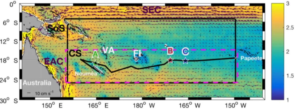
In the WTSP the large-scale circulation is dominated by the anticyclonic South Pacific Gyre. The South Equatorial Current (SEC) flows in the equatorial band (0–6◦S) from east to west and is divided into multiple branches when ap-proaching the Coral Sea (Webb, 2000; Sokolov and Rintoul, 2000) (Fig. 1). On the western boundary, the East Australian Current (EAC) feeds, through the Tasman Sea, the southern branch of the gyre which then flows east and reaches the Peru–Chile Current (PCC) near the western South Ameri-can coast (Tomczak and Godfrey, 2013). Several studies in-dicate a strong mesoscale variability, superimposed on these large-scale patterns, mostly due to barotropic and baroclinic instabilities along with interactions of major currents and jets with the numerous islands of the region (Qiu and Chen, 2004; Qiu et al., 2009; Hristova et al., 2014). As displayed in Fig. 1, the OUTPACE cruise was conducted in the tran-sition area between a zonal band of relatively high eddy ki-netic energy south of 19◦S (Qiu et al., 2009) and low eddy kinetic energy to the north. The influence of this intense vari-ability, which results in mostly westward-propagating eddies (Chelton et al., 2007; Rogé et al., 2015), has not been fully explored yet (Kessler and Cravatte, 2013), nor have its im-plications on biogeochemical/biological variations in the re-gion. Recent studies have underlined the role of mesoscale activity as a conveyor of water masses, leading to the dis-covery of a potential water mass pathway in the Coral Sea (Maes et al., 2007; Ganachaud et al., 2008; Rousselet et al., 2016). This intense mesoscale activity is strongly linked to submesoscale fronts that might be responsible for surface small-scale features in temperature and salinity as shown by Maes et al. (2013) within the Coral Sea. Submesoscale dynamics are also thought to be responsible for ∼ 20 % of new production in oligotrophic regions as suggested by Lévy et al. (2014b) using an idealized model. Since the frequency of oceanic fronts and eddy kinetic energy should increase in oligotrophic regions with climate change (Matear et al., 2013; Hogg et al., 2015) the OUTPACE cruise offers an un-precedented opportunity to study large-, meso- and subme-soscale influences along a zonal gradient crossing the olig-otrophic to ultra-oligolig-otrophic WTSP with coupled physical and biogeochemical measurements.

In this study we place the in situ observations collected during the OUTPACE cruise into a synoptic view of the WTSP circulation at different horizontal scales. We investi-gate, through a descending approach, the large-, meso- and submesoscale patterns using in situ observations, coupled

Figure 1. Mean eddy kinetic energy (log scale, colour bar) with surface velocity (arrows in cm s−1) computed for 10 years (2005–2015) from total altimetry-derived surface velocity field. The South Equatorial Current (SEC) and the western boundary East Australian Current (EAC) are indicated. The black line shows the ship track during OUTPACE from Nouméa to Papeete. The positions of the three long-duration (LD) stations are drawn with green, red and blue stars for LD stations A, B and C, respectively. SoS: Solomon Sea; CS: Coral Sea; VA: Vanuatu; FI: Fiji.

with satellite data. Remote sensing provides daily physi-cal and biologiphysi-cal information over the entire WTSP for a time period covering the cruise duration and beyond (from 1 June 2014 to 31 May 2015). The inter-comparison between physical Lagrangian diagnostics and available biogeochemi-cal/biological measurements explores the potential influence of each scale on biogeochemical variations. In particular, we propose to focus on the possible impacts of horizontal small-scale ocean circulations on horizontal distribution of temper-ature, salinity or chlorophyll, as well as on surface phyto-plankton. Two original case studies are also presented to il-lustrate the fine-scale physical influence on horizontal micro-bial distributions. The use of multidisciplinary approaches, including in situ observations, remote sensing and numerical simulations is the key aspect of this study to investigate the surface circulation at different scales and try to examine their potential influence on the distribution of biogeochemical pa-rameters and major groups of plankton measured during the OUTPACE cruise. In the following, we present the datasets and methods used and we discuss the results for each circu-lation scale, from large to submesoscale.

2 Materials and methods 2.1 In situ observations

The OUTPACE (Oligotrophy to UlTra-oligotrophy PA-Cific Experiment) cruise performed a zonal transect across the WTSP aboard RV L’Atalante from 18 February to 3 April 2015 (Moutin and Bonnet, 2015). The main objec-tives of the cruise were to study the interactions between planktonic organisms and the cycling of biogenic elements across trophic and N2fixation gradients (Moutin et al., 2017).

A total of 15 hydrological stations were sampled along the transect as well as three long-duration (LD) stations named

LDA, LDB and LDC (Fig. 1). LD station sampling lasted for almost 8 days each and aimed to study carbon export in three biogeochemically different regions. More details about the sampling strategy are available in Moutin et al. (2017). The multi-disciplinary measurements used in this study are described hereinafter.

Of particular interest to understand the surface dynam-ics, SVP (Surface Velocity Program) floats were launched during each LD station to investigate the dispersion and the surface circulation relative to 15 m during the sampling pe-riod and beyond (Lumpkin and Pazos, 2007). Three SVPs were launched during LDA, six during LDB and four during LDC. The in situ trajectories of the floats were used to val-idate altimetry-derived surface velocities (see Sect. 2.2, 2.4 and Fig. 2).

Continuous measurements of temperature and salinity were achieved using a thermosalinograph (TSG) that pumped sea water at 5 m depth. TSG data have been corrected and calibrated using independent measurements of salinity from water bottle samples collected daily onboard RV L’Atalante (following the procedures described by Alory et al., 2015) and are binned into minutes. In the following, temperature and salinity will refer to absolute salinity and conservative temperature, respectively, according to TEOS-10 standards (McDougall et al., 2012). A Wetstar Sea-Bird fluorimeter was deployed on the underway water flow. The fluorime-ter provides measurements proportional to the chlorophyll a concentration with a time step of 10–15 min. Discrete sam-ples were taken during the transit to calibrate the fluorimeter using the Aminot and Kérouel (2004) method:

Chl a [mg m−3] =1.99 × fluorescence value −0.083(R2=0.87, n = 55).

Due to technical issues the underway sampling of chloro-phyll concentration started on 7 March. Each of these data

LDA LDB LDC Geostrophy 1/4º Geostrophy 1/8º Geostrophy + Ekman 1/8º Geostrophy + Ekman + cyclogeostrophy 1/8º

Figure 2. Trajectories of numerical particles computed with Ariane (purple patch) with each satellite products and in situ floats (colours) for 8 days after the starting date of each long-duration station. The surface velocity fields of the last day of particle integration (LDA: 4 March; LDB: 23 March; LDC: 31 March) are also shown with black arrows.

sets has been interpolated on a regular grid of 0.5 km reso-lution in order to keep the high resoreso-lution, but equally dis-tributed along the travelled distance.

Two high-frequency samplings (every 20 min) were per-formed – the first one upon leaving LDA and the sec-ond one upon arriving at LDB – in order to assess vari-ability in 15 different biogeochemical parameters, in par-ticular the dissolved inorganic phosphate (DIP) turnover times and the abundances of bacteria (including the low and high nucleic acid content bacterial groups, LNA and HNA, respectively), Prochlorococcus, Synechococcus and picophytoeukaryotes (PPEs). Dissolved inorganic phosphate turnover times (TDIP) were determined using a dual14C-33P labelling method following Duhamel et al. (2006). As de-scribed in Moutin et al. (2017), TDIP represents the ratio be-tween phosphate natural concentration and phosphate uptake by planktonic species (Thingstad et al., 1993). It is consid-ered the most reliable measurement of phosphate availabil-ity in the upper ocean waters (Moutin et al., 2008). In the WTSP, the phytoplankton growth is often limited by phos-phate availability. Consequently, this parameter gives impor-tant information on the biological activity in relation to re-source availability: a very short TDIP means rapid utiliza-tion of the ambient phosphate present in limiting concen-tration. To enumerate cell abundances of these different mi-crobial groups, water samples were collected directly from the underway pump, fixed with 0.25 % (w/v) paraformalde-hyde, flash-frozen and preserved at −80◦C until analysis by flow cytometry following the protocol described in Bock et al. (2018). Briefly, bacteria were discriminated in a sam-ple aliquot stained with SYBR Green I DNA dye (1 : 10 000 final) while pigmented groups were discriminated in an un-stained sample aliquot. Reference beads (Fluoresbrite, YG, 1 µm) were added to each sample. Particles were excited at 488 nm (plus 457 nm for unstained samples) and bac-teria were discriminated based on their green fluorescence and forward scatter (FSC) characteristics, while Prochloro-coccus, Synechococcus and PPEs were discriminated based on their chlorophyll (red) fluorescence and FSC character-istics. LNA and HNA groups were further distinguished based on their relatively low and high SYBR Green fluores-cence, respectively, in a green fluorescence vs. side-scatter plot. Prochlorococcus were further distinguished from Syne-chococcus by their relative lack of a phycoerythrin signal (orange fluorescence). Using a FSC detector with small par-ticle option and focusing a 488 nm plus a 457 nm (200 and 300 mW solid state, respectively) laser into the same pinhole greatly improved the resolution of dim surface Prochlorococ-cuspopulation from background noise in unstained samples. Because the Prochlorococcus population cannot be uniquely distinguished in the SYBR stained surface samples, bacte-ria were determined as the difference between the total cell numbers of the SYBR stained sample and Prochlorococcus enumerated in unstained samples. Cytograms were analysed using FCS Express 6 Flow Cytometry software (De Novo

Software, CA, US). These data are used to investigate the small-scale distribution of the different microbial commu-nity groups and its relation with the concomitant dynam-ics at submesoscale. To investigate each picoplankton group variability with respect to the other with more clarity, abun-dances are displayed in terms of cell count deviation. The latter represents the difference between picoplankton group abundance (cell mL−1) measured at a certain location and the mean of the respective picoplankton group abundances throughout the transect.

2.2 Satellite data

Several satellite datasets were exploited during the cam-paign to guide the cruise through an adaptive sampling strat-egy using the SPASSO software package (http://www.mio. univ-amu.fr/SPASSO/, last access: 16 April 2018) following the same approach as described for previous cruises such as LATEX (Doglioli, 2013; Petrenko et al., 2017) and KEOPS2 (d’Ovidio et al., 2015). SPASSO was also used after the cruise in order to extend the spatial and temporal vision of the in situ observations.

Four different altimetry-derived velocity products were tested in this study to choose the product that best rep-resents the surface circulation during the cruise. First the daily Ssalto/Duacs product (Ducet et al., 2000), from the AVISO (Archiving, Validation and Interpretation of Satel-lite Oceanographic 3) database, for the period from 1 Jan-uary 2004 to 31 December 2015, was used to extract daily delayed-time maps of absolute geostrophic velocities (1/4◦×1/4◦on a Mercator grid, since 15 April 2014).

Three other altimetry products were specifically produced, for the first time, at 1/8◦ _{resolution for the WTSP region}

by Ssalto/Duacs and CLS (Collecte Localisation Satellites), with support from CNES (Centre National d’Études Spa-tiales), from June 2014 to June 2015. In particular, they pro-vided daily maps of absolute geostrophic velocities, daily maps of the sum of absolute geostrophic velocities and Ek-man components, and the same product as the latter that also includes a cyclogeostrophy correction (Penven et al., 2014). Ekman surface currents refer to the wind-induced circula-tion relative to 15 m and are computed from ECMWF ERA-Interim wind stress with an Ekman model fitted onto drifting buoys (Rio et al., 2014).

A preliminary comparison between Lagrangian numerical particle trajectories (see Sect. 2.3.1), computed with each of the above products, and the observed trajectories of the dif-ferent floats launched during OUTPACE (Sect. 2.1) allowed us to identify the product including geostrophic and Ekman components with the cyclogeostrophy correction (hereafter total altimetry-derived velocity field) as the most accurate in situ surface currents (see Sect. 2.4).

Daily near-real-time maps of sea surface temperature (SST) and ocean colour were also specifically produced for the WTSP from December 2014 to May 2015 by CLS

with support from CNES. They are constructed with a sim-ple weighted data average over the 5 previous days (giv-ing more weight to the most recent data), and have a 1/50◦

resolution (2 km at the Equator) in latitude and longitude. The temperature product corresponds to maps of SST de-duced from a combination of several intercalibrated in-frared sensors (AQUA/MODIS, TERRA/MODIS, METOP-A/AVHRR, METOP-B/AVHRR). The ocean colour prod-uct corresponds to maps of chlorophyll concentration is-sued from the Suomi/NPP/VIIRS sensor (http://npp.gsfc. nasa.gov/viirs.html, last access: 16 April 2018). These satel-lite data are compared with in situ data from the under-way survey. A correlation of 0.8 between in situ measure-ments and co-located satellite data validates the satellite-derived SST and chlorophyll concentration. A supplemen-tary correlation with the daily high-resolution SST blended from NCDC/NOAA (Reynolds et al., 2007) and in situ SST showed a similar correlation. These results corroborate the accuracy of the CLS products in our region of interest. 2.3 Lagrangian diagnostics

2.3.1 Surface water mass pathways detection

To investigate the water mass movements at large and mesoscale, we used the Lagrangian diagnostic tool Ariane that can trace water mass movements from the trajectories of numerical particles that enter and exit a predefined domain (Blanke and Raynaud, 1997; Blanke et al., 1999). In this study the numerical particle trajectories are computed with altimetry-derived surface currents from the products listed above (see Sect. 2.2). As many Lagrangian particles as de-sired can be integrated in two different ways: backward in time to assess the origins of the water masses or forward in time to investigate their fate. Additionally, this Lagrangian tool allows for the computation of two different diagnostics: (i) qualitative diagnostics that compute typically few parti-cles with a steady recording of the positions along their tra-jectories and (ii) quantitative diagnostics that compute thou-sands of particles with statistics available for initial and final positions, and with the diagnostic of the main pathways. In this study we use three different configurations of the Ariane tool depending on the objectives.

First, to identify the altimeter product that best fits the ob-served trajectories of the floats launched during OUTPACE, a comparison is performed, in the following Sect. 2.4, with the trajectories of 100 numerical particles. These particles were initially positioned around the launching position of the floats with a resolution of 1–2 km.

The particles were advected forward in time for 96 (LDA), 78 (LDB) and 70 (LDC) days, corresponding to the time lapse between the launch day of the floats and the last avail-able day of satellite data. These qualitative experiments al-lows for the comparison of successive positions (every 6 h) of numerical particles computed with the four different

prod-ucts and those of the floats. Thus the choice of the best sur-face velocity product relied on the best fit between observed and numerical trajectories (see Sect. 2.4).

To study the large-scale circulation in the WTSP, quantita-tive experiments were performed to find the main pathways of the waters entering and exiting the box contouring the WTSP (Fig. 3). Particles were launched along each section of the box (north, east, south, west) and advected forward with the total altimetry-derived surface currents. We simulated 10 years of particle trajectories by repeating 10 times the avail-able dataset. We compared the results of this simulation with the 10-year integration of available geostrophic AVISO sur-face currents over this time period. The comparison between these simulations ensures that the use of a 1-year time period looped several times does not significantly modify statistical outputs. It is clearly more interesting to use CLS data instead of commonly used AVISO geostrophic surface currents be-cause they include the wind effect and cyclogeostrophy with higher resolution, as well as better fitting with in situ data.

Another objective is to identify the mesoscale trajecto-ries of surface water masses sampled at each of the LD sta-tions. Backward and forward quantitative experiments were performed to identify the main pathways of the surface wa-ter masses arriving and leaving each LD station using total altimetry-derived surface currents. Almost 1 million numer-ical particles were initially distributed along a square box surrounding the position of the LD station. The calculations were stopped whenever the particles return to the initial box (hereafter called meanders) or were intercepted on one of the four remote sections located around the LD station. The boxes size are tuned in order to minimize meanders and the loss of particles in the domain. The percentage of both quan-tities are reported in Table A1 in Appendix A. Forward com-putation times are identical to the qualitative diagnostics. For backward experiments, the particles were advected for 183 (LDA), 201 (LDB) and 209 (LDC) days corresponding to the maximum time lapse allowed by CLS satellite data avail-ability.

2.3.2 Eddies and filaments identification

To set up the mesoscale context during the OUT-PACE cruise, we used the Lagrangian averaged vortic-ity deviation method (Hadjighasem and Haller, 2016; Haller et al., 2016) that allows identification of co-herent structures from altimetry-derived surface velocity fields (code available at https://github.com/Hadjighasem/ Lagrangian-Averaged-Vorticity-Deviation-LAVD, last ac-cess: 16 April 2018). The detected features are able to trap water masses for a certain period (defined by the integration time) and transport them along their route. In this study we computed the detection with the total altimetry-derived ve-locity field and chose an 8-day time integration with respect to the duration of LD stations. Indeed, this time interval pro-vides a confirmation or rebuttal of the assumption that LD

Figure 3. Total transport (Sv, colour bar) and stream function (black lines with contour interval of 0.25 Sv) computed for 10 years with the total altimetry-derived surface velocity field. The ship track and locations of OUTPACE LD stations are indicated with the black line and coloured stars as in Fig. 1.

stations have been performed in a coherent structure, as tar-geted during the cruise. This Lagrangian diagnostic is also compared with a hybrid Lagrangian and Eulerian approach combining the calculation of the Okubo–Weiss (OW) param-eter and a retention paramparam-eter (RP), computed with the same velocity field. The OW parameter identifies structures such as eddies by separating the flow into a vorticity-dominated region and a strain-dominated region (Okubo, 1970; Weiss, 1981). The RP identifies the number of days a fluid parcel re-mains trapped within a structure core, defined by a negative OW parameter. Both parameter calculations are detailed in d’Ovidio et al. (2013). As for the LAVD detection method, the RP allows for the identification of potentially trapping coherent structures.

Submesoscale flow features in two-dimensional data are evaluated with altimetry-derived finite size Lyapunov expo-nents (FSLE), computed with the algorithm of d’Ovidio et al. (2004). This Lagrangian diagnostic detects frontal zones on which passive elements of the flow should theoretically align. Here we used the total altimetry-derived velocity field to compute the algorithm. The main parameter values for the algorithm are described in de Verneil et al. (2017). The OUT-PACE cruise occurred in the relatively open ocean and far enough from islands to trust the FSLE diagnostic calculated from altimetry.

We compare the horizontal positions of the fronts, de-tected with FSLE, with surface gradients measured both with the TSG (temperature and salinity) and the underway sur-vey (chlorophyll). Indeed, these high-frequency samplings provide access to submesoscale gradients. A point-by-point correlation is calculated whenever a strong gradient of den-sity (or chlorophyll) corresponds or not to a high FSLE value (i.e. > 0.05 day−1) indicative of a front. Sensitivity tests have been performed to choose the thresholds on density (chlorophyll) gradients to ensure the stability of the correla-tions calculated. These tests ended with the selection of gra-dient larger than 0.1 kg m−3km−1 and a 0.2 mg m−3km−1

as thresholds for density and chlorophyll gradients, respec-tively.

2.4 Comparison of satellite products with in situ drifters

The choice of the satellite product that best represents the surface dynamics relies on a qualitative comparison between the trajectories of in situ floats launched during the OUT-PACE cruise (see Sect. 2.1) and the trajectories of numerical particles computed with each of the satellite-derived velocity field described in Sect. 2.2. Figure 2 shows the 8-day trajec-tories of in situ floats and numerical particles at each long-duration station and for each satellite-derived products con-sidered (geostrophy 1/4◦_{; geostrophy 1/8}◦_{; geostrophy and}

Ekman 1/8◦_{; geostrophy, Ekman and cyclogeostrophy 1/8}◦_).

The comparison is restricted to 8 days for a better visualiza-tion and to be consistent with the duravisualiza-tion of the LD stavisualiza-tions. In the case of station LDA, none of the products displays a significant improvement of numerical trajectories. This lack of refinement between the different products may be due to the lack of accuracy of satellite products when getting close to coasts. Indeed, altimetry measurements are not well re-solved close to the coast, and especially near New Caledonia, where the topography and bathymetry are very complex. In the cases of LDB and LDC, the increase in resolution does not modify the general pattern of the trajectories. However, when adding the Ekman component, we can notice an im-provement in the direction of the numerical particle trajecto-ries. Even if the particle positions are offset, their direction are consistent with those of in situ drifters. Cyclogeostrophy seems to accelerate the particles’ displacements. The final positions of the numerical particles are closest to the final po-sition of in situ drifters in the case of LDC. This latter point is not surprising considering that cyclogeostrophy represents the centrifugal acceleration. In the context of the OUTPACE cruise, we consider that the LDB and LDC examples illus-trate clear improvements of the new satellite product

includ-ing geostrophy, the Ekman component and cyclogeostrophy. In the case of LDA neither clear improvement nor deteriora-tion is obvious on the trajectories. Moreover, when consider-ing the surface circulation, it also remains important to take into account the wind effect, through the Ekman component, as it will strongly influence the trajectories of surface waters at large, meso- and submesoscale. As most of the diagnos-tics used in this study are calculated through particle trajec-tory computations, the Ekman component is of major sig-nificance. As a consequence, and to stay consistent through-out this study, we used the product combining geostrophy, the Ekman component and cyclogeostrophy at 1/8◦ resolu-tion, referred to as the total surface altimetry-derived velocity field, to compute every diagnostic.

3 Results and discussions

3.1 Large-scale wind-driven pathways

The geostrophic large-scale mean circulation and directions of the main currents in the WTSP are well established from the literature. However, the trajectories and pathways of sur-face waters may change and be more complex when the effect of the wind is added and resolution is increased es-pecially in the context of inter-annual ENSO (El Niño– Southern Oscillation) variability. We decided to use a La-grangian integration of numerical particles to simulate the transport of surface fluid parcels at the scale of the WTSP region using altimetry-derived ocean currents including the wind effect. Figure 3 shows the transport calculated from the sum of almost 13 million numerical particles advected with the total surface altimetry-derived flow for 10 years (see Sect. 2.3.1). This figure highlights the westward transport of the SEC in the northwestern part of the domain, as well as the eastward transport at 10◦S due to the output of the South Equatorial Countercurrent (SECC) from the Solomon Sea (Ganachaud et al., 2014). Both these pathways follow the well-known circulation of the SEC and SECC in this region. An eastward flow south of Fiji is also detectable in Fig. 1 but does not seem to influence surface transport (Fig. 3). This flow has been discussed in several studies and is named the South Tropical Countercurrent (STCC) (Qiu and Chen, 2004). Additionally, a clear surface meridional transport is noticeable from 10 to 25◦S. In the very southeastern part of the domain some surface waters seem to recirculate to the east from 170◦_{W, which is probably an indicator of the gyre}

circulation. The meridional transport does not correspond to any general surface geostrophic current previously described in the literature (Tomczak and Godfrey, 2013; Kessler and Cravatte, 2013; Ganachaud et al., 2014) but is mainly due to the south-easterly trade winds. This meridional compo-nent appears due to the addition of the Ekman compocompo-nent in altimetry surface velocities (Fig. A1, Appendix A). The large-scale transport of surface waters in the OUTPACE area

is thus a combination of the transport by general well-known surface currents and wind-driven circulations. Most of the surface waters travel southwest from the northern Ariane sec-tion, with a significant part that originates from northeast. At the scale of the WTSP, the individual transport calculated from each initial section (see Sect. 2.3.1) reveals that 80 % of the surface waters crossed during the OUTPACE cruise origi-nate from the “north” section, 8–15 % from the “east” section and very few from the “south” and “west” sections (Fig. A2). We can thus identify a general wind-driven surface transport in the WTSP as follows: the surface waters enter the WTSP from the northeast with the SEC and are gradually advected to the south with a part (east of 170◦W) that directly recir-culates within the gyre and another part (west of 170◦W) that follows a southwestern propagation through the differ-ent WTSP archipelagos. These results obtained with a La-grangian diagnostic complete the largely elucidated Eulerian vision of the large-scale circulation in the WTSP.

Very few reports have studied the surface transport in-ferred by the wind in the WTSP. Indeed, Tomczak and God-frey (2013) calculated a stream function from wind stress and showed a global westward transport with very little merid-ional transport except in the EAC, which is very close to the Australian coasts. Kessler and Cravatte (2013) also com-puted the Sverdrup transport stream function calculated from Godfrey’s island rule and the wind stress curl field in the Coral Sea. They identified a comparable southward trans-port as visible in Fig. 3, between 7 and 12◦S, due to the SECC. However, between 12 and 25◦S, they identified a westward transport whereas we show a meridional trans-port from north to south. Considering the large-scale biogeo-chemical distribution, two types of waters can be differenti-ated: the relatively oligotrophic but richer Melanesian waters (from 160◦E to 170◦W) and the ultra-oligotrophic gyre wa-ters (east of 170◦W) (Fumenia et al., 2018). The wind-driven surface transport highlighted here could participate in the biogeochemical variations between western and eastern wa-ters. Moreover, the path through the Melanesian area, which includes the multiple islands from Papua New Guinea to Fiji (140◦E–170◦W), may enrich these waters due to the con-tact with multiple islands. This could explain the relatively higher productivity of these waters, whereas waters that di-rectly recirculate within the gyre keep their ultra-oligotrophic characteristics.

The WTSP circulation is also strongly impacted by ENSO conditions, responsible for SST variability on inter-annual to decadal timescales (Sarmiento and Gruber, 2006). A nega-tive Southern Oscillation index (SOI), El Niño phase, is char-acterized by a decrease or even an overturn of trade winds whereas during La Niña phase (positive SOI) trade winds are strengthened. The mean wind velocity measured during OUTPACE is shown to be close to mean velocities during El Niño (data not shown) and Moutin et al. (2017) clearly showed that the OUTPACE cruise took place during an El Niño phase, but they determined that climatological effects,

Figure 4. Daily sea surface level anomaly (m, colour bar) and velocity field (m s−1) from the total altimetry-derived surface product for the first day of LDA (25 February, a), LDB (15 March, b) and LDC (23 March, c). Contours of LAVD-detected structures are drawn in green. The centre of the structures is also indicated by a green point. The ship track and locations of OUTPACE LD stations are indicated with the black line and coloured stars as in Fig. 1.

upon the results of the cruise, were minimized for biogeo-chemical sampling. However we show that the circulation and transport are still strongly influenced by the trade winds. As this region is characterized by an intense mesoscale cir-culation, we can also expect that it participates in the bio-geochemical variations in the region. Thus we investigate the mesoscale feature trajectories on the entire WTSP and in par-ticular the mesoscale circulation around three biogeochemi-cally different locations: (i) LDA, located in the Coral Sea, at the end of the surface waters’ journey across the WTSP; (ii) LDB, in the Melanesian waters, west of the transition zone with gyre waters; and (iii) LDC, in the gyre waters. 3.2 Mesoscale activity and trajectories of

surface waters

The major goal in this section is to identify whether mesoscale activity, and in particular trapping features, ac-tively participates in the transport of different water mass properties across the WTSP. The LAVD method is chosen in order to track the coherent structures for a time period of 8 days (see Sect. 2.3.2). Figure 4 shows the total altimetry-derived velocity field and the mesoscale structures identified for the first day of each LD station (LDA, LDB and LDC). It reveals that many mesoscale structures are detected by the LAVD method in the entire WTSP with no specific

re-gion with higher abundances of these features. To ensure that this recent detection method is consistent with previous ap-proaches that identify mesoscale features (Eulerian Okubo– Weiss parameter) or retention areas (RP), we compare the structures detected with both approaches. A comparison with the OW parameter method shows a good agreement with the LAVD detection method. Indeed, a mean OW parame-ter value of −0.24 day−2is calculated inside the contour of coherent structures detected with the LAVD method. It in-dicates that wherever a coherent structure is identified, the OW parameter also identifies a mesoscale feature. Most of the mesoscale structures detected with the LAVD method are also identified as retention areas, with the RP, ensuring the trapping characteristics of these features (Fig. A3). A track-ing of these coherent structures highlights that they all show a general westward propagation as expected from the mean circulation in this area.

Coherent mesoscale features are well known to partici-pate in the surface biogeochemical variations through eddy trapping and transport. Unfortunately, in our case, we are not able to observe the trapping and transport of different water masses by the mesoscale structures with in situ data. Indeed, the zonal equidistant biogeochemical sampling dur-ing OUTPACE did not sample both mesoscale features and surrounding waters. Consequently no differentiation is

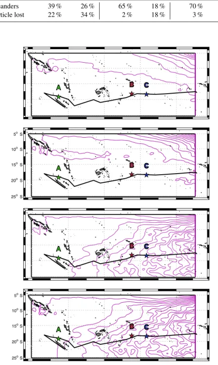
possi-Figure 5. Backward (a) and forward (b) stream functions for LDA (green lines), LDB (red lines) and LDC (blue lines). Numerical particles are initially launched on the magenta boxes which represent the position of each LD station. The domain limit of each Ariane Lagrangian analysis is shown by the large green, red and blue boxes respectively. The ship track of OUTPACE is indicated with the black line.

ble between potentially trapped waters and surrounding wa-ters. The small differences between water mass properties in this region (Gasparin et al., 2014) may also make it diffi-cult to confidently notice a biogeochemical marker of dif-ferent water masses. Even if, in this case, the influence of mesoscale activity, through eddy trapping and transport, on biogeochemical variations is not directly visible on in situ data, the role of mesoscale dynamics on the trajectories of surface waters can document the possible exchanges between biogeochemically differentiated regions.

Here we also dynamically explore the origins and fates of surface waters sampled during each LD station located in three different environments. LDA is situated on the path of the westward North Caledonian Jet (NCJ), which flows be-tween New Caledonia and Vanuatu, in relatively highly pro-ductive waters (Fig. 6). Far to the east, LDB is positioned near the limit between oligotrophic and ultra-oligotrophic waters inside a phytoplankton bloom whereas LDC is located in nutrient-poor waters in the South Pacific (SP) gyre (Fig. 6). Figure 5 shows the stream functions calculated from numer-ical particle advection using total altimetry-derived surface velocities (see Sect. 2.3.1). These stream functions represent the origin (Fig. 5a) and the fate (Fig. 5b) of each LD stations’ waters, respectively the backward and forward computations. One would expect LDA surface waters to come from the east as it is located on the path of the westward NCJ. However they seem to have multiple origins: (i) easterly, directly from the NCJ transport; (ii) northerly, directly from waters that have circulated between the Vanuatu islands before heading south to LDA; and (iii) from a meridional tortuous

recircula-tion path (∼ 162◦E) within the Coral Sea. After LDA sam-pling, an intense signature of the NCJ is detected at the sur-face. Another portion of surface waters directly crash on New Caledonia’s northern coast. In the eastern WTSP, LDB sur-face waters seem to follow the same general path: they flow from northeast towards southwest before they reach a group of islands and then recirculate to the east towards LDB. Af-ter LDB sampling, they continue their way to the east before heading back to the south or to the south-west. Further east, as one would expect, the waters sampled during LDC trav-elled from the east and flow to the west after LDC (Fig. 5). We notice a recirculation area east of LDC where the waters seemed to follow a looping trajectory before reaching LDC. Both Lagrangian methods (LAVD detection and advection of numerical particles) detect a coherent mesoscale structure that travelled westward in the surrounding region of LDC.

The identification of coherent structures during OUT-PACE revealed that only station LDC could be influenced by a trapping structure. A tracking of this structure, as well as the high rates of meanders (70 and 44 % for backward and forward integration, respectively) (Table A1), suggests that this coherent structure crossed the LDC sampling area. Indeed, some CTD casts were performed inside or near the boundary of this structure, whereas others, mostly at the end of the station, were realized after the crossing of the struc-ture. This observation can be associated with the results of de Verneil et al. (2018), who identified, with in situ data, a modification in the water mass composition throughout the station. We thus suggest that the change in the physical envi-ronment during LDC could be due to the westward transit of

Figure 6. (a) Lagrangian satellite sea surface temperature (◦C) (for the time period of the OUTPACE cruise, adapted from de Verneil et al., 2017) from CLS superimposed with 5-day weighted mean of sea surface temperature (◦C) from TSG (coloured circles with centres indicated in white). (b) Lagrangian satellite-derived surface chlorophyll concentration (mg m−3) (for the time period of the OUTPACE cruise, adapted from de Verneil et al., 2017) from CLS superimposed with 5-day weighted mean of surface chlorophyll concentration (mg m−3) measured onboard during OUTPACE (coloured circles with centres indicated in white). Fronts are present for at least 10 days during the OUTPACE cruise are indicated in grey in both figures. (c) Recurrence of FSLE structures (number of days of FSLE presence, colour bar).

this coherent structure across LDC sampling site. Although only the trajectories at the LDC sampling site seem to show a direct influence of water mass transport through coherent mesoscale structure, the trajectories at LDA and LDB still highlight some interesting mesoscale paths (circulation at the scale of the order of 10–100 km). Around LDA, both (i) and (ii) origins agree with the integrated transport entering the Coral Sea induced by the complex topography (Kessler and Cravatte, 2013). The westward circulation scheme is consis-tent with previous studies focusing on the NCJ (Ganachaud et al., 2008; Gasparin et al., 2011) and more consistently with the results analysed by Barbot et al. (2018) within the same context and cruise. The pathway that crashes on New Caledo-nia’s coast might not be so relevant due to the satellite’s lack of resolution near coastal areas. The meridional recirculation previously determined suggests that eddy–eddy interactions might be responsible for the emergence of complex paths be-tween the NVJ (North Vanuatu Jet) and the NCJ. Moreover, backward and forward stream functions cross around station LDA, which suggests that the area between New Caledonia and Vanuatu is a region of complex recirculation with waters that stay in this region for a while before exiting the Coral Sea. These observations match the area described by

Rous-selet et al. (2016) as the region of exchange between NCJ and NVJ waters through eddy trapping and transport. We identify a probable water mass mixing area, in the Coral Sea centre, through complex mesoscale stirring. This stirring may also create surface gradients as depicted by Maes et al. (2013). Around LDB, an eastward path is detected that could match with the eastward flow of the STCC. Moreover, de Verneil et al. (2017) also pointed out a possible eastward transport to explain the origin of the bloom sampled at LDB. Indeed, the surface waters might be iron-enriched through contact with the islands and thus create favourable conditions for a phyto-plankton bloom. At this site, adjacent to the nutrient-poor SP gyre, the biological dynamics could be specially enhanced by the mesoscale eastward transport of essential chemical sup-plies for phytoplankton development. If this mesoscale east-ward transport is revealed to be quasi-permanent, it could be associated with recurrent bloom events in this area, but this assumption requires further analyses to be generalized. 3.3 Fine-scale distribution of tracers

The surface tracers’ distribution is mostly driven by the wind-induced circulation but also by the transport through

mesoscale activity. In a more ephemeral way, tracers can be dispersed following small-scale perturbations such as frontal features. Here we aim to detect and quantify the influence of such features on the density and chlorophyll surface gradi-ents using both in situ and satellite observations.

As described in Sect. 2.2 and shown by Fig. 6a and b, the comparison between in situ observations and satellite-derived data results in reasonable correlations. The differ-ences between in situ temperature (top), chlorophyll (bottom) and satellite data are plotted in Fig. A4. We obtain differ-ences between +1.5 and −1◦C which allows us to confi-dently use satellite temperature. For chlorophyll, the differ-ences are smaller than ±0.1 mg m−3which is also a reason-able deviation between satellite and in situ measurements, besides considering the colour bar scale of Fig. 6 with values that vary from 0 to 1 mg m−3. We can also note that the satel-lite data clearly underestimate chlorophyll concentrations in the Melanesian area. As both datasets are comparable, SST and chlorophyll concentrations from remote sensing are then used to investigate horizontal gradients in the WTSP (Fig. 6a and b). To assess the spatial scale of submesoscale gradi-ents (typical of 1–10 km) in terms of ocean dynamics, we use a Lagrangian methodology based on the calculation of FSLE (see Sect. 2.3.2) that allow for front detection. Fig-ure 6c shows regions where fronts are frequently generated during the time period of the cruise. We notice that the gyre is a region less suitable for fronts to occur and persist. East of the Fiji islands we also identify a zonal band at 18◦S, where almost no fronts occur during the OUTPACE cruise. South-east of LDB a mesoscale structure, which is also identified in Fig. 4, creates a frontal barrier that lasted for more than 30 days. It seems that this structure matches with strong sur-face gradients in chlorophyll and in SST, consequently sep-arating colder and relatively chlorophyll-rich waters to the south from warmer but chlorophyll-poor waters to the north of the front. Overall, as shown by Fig. 6, the most frequent and long-lived fronts seem to help in structuring the spatial distribution of tracers such as SST and chlorophyll concen-tration by creating physical barriers, isolating areas with dif-ferent biogeochemical characteristics. To try to quantify the influence of frontogenesis on the structuring effect of surface tracers, we decided to compare the surface sharp gradients measured by the TSG or with the underway fluorimeter with the presence of a front detected from the total surface satellite product.

The strong surface density gradients (as defined in Sect. 2.3.2) represent 9 % of the data measured by the TSG during the OUTPACE cruise. The comparison with FSLE re-veals that 25 % of the strong surface density gradients match with a physical front. Through a bootstrapping re-sampling, the same method is applied to the 91 % of TSG data identi-fied as non-gradient and demonstrates that only 14 ± 1 % of homogeneous density areas match with a front. These latter results also show that an FSLE existence does not necessar-ily create a gradient but probably needs pre-existing tracer

gradients and a lifetime longer than few days. The same calculations have also been performed for temperature and salinity gradients independently and show similar results. The relatively better correlation between density gradients and FSLEs than between no-density gradients and FSLEs attests that gradients are not randomly distributed with re-gard to FSLE structure and proves that FSLE detection can be a good candidate to explain the presence of in situ surface gradients. The same approach was performed with a reac-tive tracer, the chlorophyll concentration sampled with high frequency. It shows that 35 % of strong surface chlorophyll gradients, representative of 1 % of the entire underway sam-pling, agree with the presence of FSLE. Re-sampling over the 99 % of non-gradient areas indicates that 28 ± 14 % of homogeneous chlorophyll areas match with an FSLE.

The correlations with FSLE are not high enough to clearly demonstrate that physical front structure the entire surface distribution of tracers. However they give a relative confi-dence on the fact that they can structure the surface tracers’ distribution. The relative orientation of the front with respect to the direction of the density gradient can also be a factor that controls the generation of a strong gradient. The zonal characteristic of the OUTPACE section forces the surface gradient identified with the TSG to be mainly representative of cross track fronts. Moreover, the lack of precision of the calculation method may also cause a decrease in the corre-lations calculated. Despite the effort to increase the altime-try resolution to 1/8◦, it is still not enough to fully resolve the submesoscale gradients. Consequently the correlation be-tween surface gradients and FSLE can probably not increase much higher than the 25 % calculated here. This result con-verges with Hernández-Carrasco et al. (2011), who showed that FSLEs can still give an accurate picture of Lagrangian small-scale features despite some missing dynamics. Addi-tionally, our method relies on a comparison between absolute values of gradients and co-located FSLE. Due to the lack of resolution of satellite products, this point-by-point com-parison may induce an offset of a few kilometres between the area identified with FSLE and the gradient sampled with the TSG. Consequently, the method applied here may not identify the match. Therefore, the methodology could be im-proved by focusing on FSLE values around a certain radius from the position of the gradient to eliminate the uncertainty caused by the absolute point-by-point comparison. Another way to improve the method would be to only take into ac-count cross-front gradients that are more likely to be induced by a physical front than along-front gradients. However, con-sidering that the SST distribution is also governed by other processes than advection, such as the diurnal cycle, the 25 % correlation is large enough to sustain the idea that the sub-mesoscale circulation can participate actively in the spatial structuring of surface tracers such as sea surface salinity, SST or density. Concerning the biological chlorophyll parameter, the high percentage (28 %) of FSLEs matching with a “no-chlorophyll-gradient” area gives little confidence in the fact

Figure 7. (a) Chlorophyll concentration (mg m−3, colour bar) from 13 March 2015 superimposed with bacteria counts (cell mL−1, red-blue colour bar) sampled during LDB. FSLE fronts (val-ues > 0.05 day−1) are shown in grey. The location of LDB is indi-cated with the red star. White squares are missing satellite data due to cloud cover. (b) Cell count deviation (see Sect. 2.1) of Prochloro-coccus, SynechoProchloro-coccus, PPEs and bacteria (HNA and LNA) super-imposed with FSLE (day−1, black line), surface chlorophyll con-centration (µg L−1, green crosses) and dissolved inorganic phos-phate turnover time (hours, orange stars) along the high-frequency transect of LDB.

that 35 % of chlorophyll gradients were actually caused by the presence of a physical barrier. As chlorophyll concentra-tion is driven by many biological processes, it may be more accurate to associate gradients of phytoplankton abundances, responsible for chlorophyll gradients, with small-scale fea-tures. Hereinafter, using two case studies of plankton high-frequency sampling, we propose to compare microbial abun-dances with frontal features.

3.4 Example of physical barriers’ influences on phytoplankton community

In this section we present two case studies that highlight the potential influence of fronts on phytoplankton horizontal dis-tribution. To test the hypothesis of Bonnet et al. (2015), who pointed out the use of FSLE to explain some correlations between Trichodesmium spp. abundances and gradients, we measured the abundances of microbial groups of plankton in samples collected during two high-frequency sampling tran-sects (Figs. 7 and 8). LDB high-frequency sampling crosses from north to south the bloom patch described in de Verneil et al. (2017). The spatial distribution of organisms presents relatively high concentration of bacteria at the centre of the bloom but decreases when exiting this feature (Fig. 7). An FSLE barrier is visible near the centre of the transect. This barrier coincides with what is identified as a strong density gradient by our methodology, depicted in Sect. 3.3. It is also associated with a sharp decrease in surface chlorophyll con-centration (Fig. 7b). The variations in the abundance of Syne-chococcus, HNA and LNA (bacteria in general) follow the pattern of surface chlorophyll. We can also notice a slight de-crease in PPE abundance to the south of the front. Prochloro-coccus show different variations: the abundance seems to increase when crossing the front and then decreases to the south of it. There is a sharp increase in TDIP when exiting the patch in the south, indicating that phosphorus is quickly consumed inside the bloom. The front thus seems to create a barrier for certain organisms which grow and accumulate on one side of the front as demonstrated by relatively high surface chlorophyll (peak at 0.8 µg L−1) and low phospho-rus. For LDA high-frequency sampling (Fig. 8a), we can notice a region of high abundance of bacteria at 165◦₁₅0_E

bounded by two FSLE barriers. This trend is confirmed by Fig. 8b, which shows a relative increase in the abundance of Prochlorococcus, bacteria, HNA and LNA associated with a spike of FSLE values at 45 km. Interestingly, the abundance of PPEs seems to decrease where bacterial abundances are the highest, indicating that conditions favouring bacteria and picocyanobacteria are not necessarily favourable to PPEs. In contrast, another FSLE peak at 75 km was characterized by the decrease in Prochlorococcus, bacteria, HNA and LNA while the PPE abundance increases. The surface chlorophyll follows the same pattern as that of Prochlorococcus, bacteria, HNA and LNA with a relative increase in chlorophyll con-centration (∼ 0.3 µg L−1) within the region bounded by the FSLEs. However, Synechococcus abundance does not show any variations that coincide with submesoscale features. An-other peak in chlorophyll concentration is noticeable around 30 km (∼ 0.4 µg L−1) but may be associated with other or-ganisms than those analysed with cytometry.

The previous observations suggest that physical barriers to transport, detected with FSLE, can influence phytoplank-ton community structure by separating or concentrating dif-ferent picoplankton group. In the LDB case study, the front

Figure 8. (a) Chlorophyll concentration (mg m−3, colour bar) from 3 March 2015 superimposed with bacteria counts (cell mL−1, red-blue colour bar) sampled during LDA. FSLE fronts (val-ues > 0.05 day−1) are shown in grey. The location of LDA is in-dicated with the green star. White squares are missing satellite data due to cloud cover. (b) Cell count deviation (see Sect. 2.1) of Prochlorococcus, Synechococcus, PPEs and bacteria (HNA and LNA) superimposed with FSLE values (day−1, black line) and sur-face chlorophyll concentration (µg L−1, green crosses) along the high-frequency transect of LDA.

seems to act like a barrier along which some picoplankton groups aggregate with weak possibilities to cross the front. As a consequence, bacteria and phytoplankton grow on one side of the front, whereas, on the other side, the abundances are quite low. According to Mann and Lazier (2013) phyto-plankton growth may be stimulated in aggregates, where they can easily take up nutrients released by bacterial decompo-sition of organic matter. This phenomenon may explain why the abundance is more important on one side of the front. It may also support the persistency of the bloom during LDB. Indeed, the bloom may be sustained in time by submesoscale features creating an aggregation of microorganisms that can benefit from each other. de Verneil et al. (2017) identified the influence of the mesoscale horizontal processes in generating the bloom. They also showed that the bloom was bounded by

some physical features acting like barriers. The results pre-viously presented in this paper support the significance of horizontal submesoscale processes in driving the bloom’s dy-namic. Here we show that the distribution of phytoplanktonic community inside the bloom is conditioned by submesoscale features.

Our case study at LDB indicates that submesoscale fea-tures could create favourable conditions for certain plankton groups at the expense of others. A similar phenomenon oc-curs at LDA: the abundances of PPEs decrease inside the region bounded by FSLEs where bacterial abundances in-crease. This observation probably indicates that PPEs may not find an advantage in these features. Thus the physi-cal fronts not only structure the spatial distribution of or-ganisms by creating barriers but also seem to create bor-der regions influencing the community structure, abundances and diversity. Indeed, modelled fine-scale structures have al-ready been shown to delimit niches of different phytoplank-ton types but also to modify phytoplankphytoplank-ton assemblages and diversity (d’Ovidio et al., 2010; Lévy et al., 2014a). Con-sistent with these previous numerical results, our in situ ob-servations show that microbial growth may benefit from the horizontal conditions engendered by frontal structures. Mar-rec et al. (2018) also Mar-recently observed a peculiar distribu-tion of phytoplankton types inside and outside a mesoscale structure, demonstrating the structuring effect of meso- and submesoscale dynamics on phytoplankton communities. It is also interesting to note that, for our case studies, some pi-coplankton groups’ horizontal distribution is not necessarily impacted by the presence of submesoscale features, as for Synechococcusduring LDA, or respond with a different dy-namic, as for Prochlorococcus during LDB. This observation demonstrates that physical features are a key component but not the only parameter that drives the horizontal variations of phytoplankton communities. Indeed, some patterns can also be explained by inherent biological dynamics. In the con-text of the OUTPACE cruise, it thus remains important to investigate the role of N2-fixing organisms during these two

case studies and to determine how the organisms involved in N2fixation respond to the presence of submesoscale features

(Bonnet et al., 2015).

4 Conclusions

We document here the surface circulation at different spatial scales (from 1000 down to a few kilometres) and its influ-ence on horizontal dispersal of biogeochemical components in the WTSP during the OUTPACE cruise. This study is conducted thanks to the combined use of value-added high-resolution altimetry products, in situ observations and La-grangian numerical simulations. The total altimetry-derived velocity field, combining geostrophy and wind components, revealed a wind-driven meridional pathway of surface wa-ters in the WTSP. This surface trajectory can be linked to the

biogeochemical differences between Melanesian waters and gyre waters: a part of the water masses directly recirculates into the gyre, whereas the other part is driven across multiple islands of the WTSP.

The mesoscale activity is confirmed to be intense and mostly westward. Most of these mesoscale structures demon-strated ability to trap waters; however, no obvious biogeo-chemical variations were linked to eddy entrapment. We identify two areas where the mesoscale circulation might have a strong influence on water mass transport. First, the central Coral Sea appears as a region of exchange between distinct NVJ and NCJ waters through eddy transport. Second, the band between 180 and 170◦W could emerge as a recur-rent bloom formation area due to the simultaneous effect of N2 fixation, well known to sustain summertime blooms in

the WTSP, and the eastward mesoscale transport of waters nutrient-enriched due to the contact with islands.

Associating the surface small-scale gradients with La-grangian diagnostics of frontal features, we showed a corre-lation of at least 25 %, highlighting the role of submesoscale activity in governing the horizontal dispersal of surface trac-ers. The small-scale features also participated in the horizon-tal distribution and community structure of phytoplankton patches sampled during two original high-frequency sam-pling of surface phytoplankton abundances.

Future studies in the area will need to take into account the interactions between physical features of the flow at large and fine scales to better understand the phenomenon that drives the distribution of buoyant matter. In particular, the re-gion around station LDB should be investigated during other bloom events to confirm the possible role of enriched-water mesoscale transport in instigating/driving the bloom. This study also revealed the necessity to perform high-frequency sampling during oceanographic cruises to fully resolve sub-mesoscale impacts on biogeochemical distributions.

Data availability. All data and metadata are available at the French INSU/CNRS LEFE CYBER database (scientific coor-dinator: Hervé Claustre; data manager and webmaster: Cather-ine Schmechtig) at the following web address: http://www.obs-vlfr. fr/proof/php/outpace/outpace.php (INSU/CNRS LEFE CYBER, 2017).

Appendix A

Table A1. Percentage of particles that return to the initial box (meanders) and percentage of particles that do not reach any controlled sections during the integration (lost) for each backward and forward Lagrangian experiments around LD stations.

STATION LDA LDB LDC

Backward Forward Backward Forward Backward Forward Meanders 39 % 26 % 65 % 18 % 70 % 44 % Particle lost 22 % 34 % 2 % 18 % 3 % 2 % AAA BBB CCC 156oE 168oE 180oW 168oW 156oW 25o_S 20o_S 15o_S 10o_S 5o_S A_AA BBB CCC 25oS 20oS 15o_S 10oS 5oS AAA BBB CCC 25oS 20o_S 15o_S 10oS 5o_S A_AA BBB CCC 25oS 20oS 15o_S 10oS 5oS 156o_{E 168}o_{E 180}o_{W 168}o_{W 156}o_W 156oE 168oE 180oW 168oW 156oW 156o_{E 168}o_{E 180}o_{W 168}o_{W 156}o_W

Figure A1. Forward stream functions computed for a 10-year period with, from top to bottom, the low-resolution geostrophic product of AVISO; the high-resolution geostrophic product from CLS; the high-resolution geostrophic and Ekman (at 15 m) product from CLS; and the high-resolution geostrophic, Ekman (at 15 m) and cyclogeostrophic product from CLS (referred to as the total altimetry-derived product in the text). The initial section of Ariane Lagrangian analysis is indicated with a purple vertical line to the east. The ship track and locations of OUTPACE LD stations are indicated with the black line and coloured stars as referred to in Fig. 1.

A

B

C

Figure A2. Forward stream functions computed for a 10-year period with the total altimetry-derived product from CLS. Each streamline’s colour corresponds to the initial section of numerical particles: north section (orange lines), east section (purple lines), south section (green lines) and west section (magenta lines). The ship track and locations of OUTPACE LD stations are indicated with the black line and coloured stars as in Fig. 1.

Figure A3. Particle retention time (days, colour bar) and velocity field (m s−1) derived from the geostrophy, Ekman and cyclogeostrophy included product for the first day of LDA (25 February, a), LDB (15 March, b) and LDC (23 March, c). Contours of LAVD-detected structures are drawn in green. The centre of the each structure is marked with a green point. The ship track and locations of OUTPACE LD stations are indicated with the black line and coloured stars as in Fig. 1.

A

B

_C

A

B

_C

Figure A4. (a) Difference between in situ surface temperature from TSG and satellite-derived sea surface temperature from CLS (◦C). (b) Difference between in situ surface chlorophyll concentration from the underway survey and satellite-derived sea surface chlorophyll concentration from CLS (mg m−3).