Sizing of a short term wind forecasting system

(1)

HAL Id: tel-02513065

https://tel.archives-ouvertes.fr/tel-02513065

Submitted on 20 Mar 2020

HAL is a multi-disciplinary open access

archive for the deposit and dissemination of sci-entific research documents, whether they are pub-lished or not. The documents may come from teaching and research institutions in France or abroad, or from public or private research centers.

L’archive ouverte pluridisciplinaire HAL, est destinée au dépôt et à la diffusion de documents scientifiques de niveau recherche, publiés ou non, émanant des établissements d’enseignement et de recherche français ou étrangers, des laboratoires publics ou privés.

Sizing of a short term wind forecasting system

Aurore Dupre

To cite this version:

Aurore Dupre. Sizing of a short term wind forecasting system. Geophysics [physics.geo-ph]. Institut Polytechnique de Paris, 2020. English. �NNT : 2020IPPAX002�. �tel-02513065�

(2)

626

NNT

:2020IPP

AX002

Sizing of a short term wind forecasting

system

Th`ese de doctorat de l’Institut Polytechnique de Paris

préparée à l’ École polytechnique École doctorale n◦_{626 École Doctorale de l’Institut Polytechnique de Paris (IP Paris)} Spécialité de doctorat : Météorologie, océanographie physique et physique de l’environnement

Thèse présentée et soutenue à Palaiseau, le 22 janvier 2020, par

A

URORE

D

UPRE

´

Composition du Jury :

Mathilde Mougeot

Professeur, ENSIIE Pr´esident

Antoine Rousseau

Directeur de recherche, Inria - Montpellier Rapporteur Freddy Bouchet

Directeur de recherche, ENS - Lyon Rapporteur

B´en´edicte Jourdier

Ing´enieur de recherche, EDF R&D Examinateur

Mireille Bossy

Directeur de recherche, Inria - Sophia Antipolis Examinateur Philippe Drobinski

Directeur de recherche - LMD Directeur de th`ese

(3)

(4)

(5)

4

Dimensionnement d’un système de prévision éolienne à court terme

Résumé – Dans un contexte de réchauffement climatique et de transition énergétique, le développement des énergies renouvelables est indispensable afin de garantir une production d’énergie qui réponde à une demande en croissance constante. Cependant, l’intermittence de ces ressources reste un frein quant à leur pénétration. Avoir accès à des prévisions court terme fiables est essentiel et c’est d’autant plus le cas pour l’éolien qui dépend d’une ressource extrêmement variable.

Les producteurs éoliens Français bénéficient d’une période de rachat obligatoire de leur produc-tion de la part d’EDF durant 15 ans. Après cela, ils doivent vendre leur producproduc-tion sur le marché concurrentiel. Pour ce faire ils doivent annoncer à l’avance la quantité d’énergie qu’ils injecteront sur le réseau. En cas de déséquilibre, des pénalités leurs sont imputées. Ainsi, anticiper de manière précise la quantité d’énergie produite permet de maximiser le revenu. En France, l’échéance limite pour vendre son énergie est de 30 minutes. Ainsi, dans cette thèse, plusieurs approches de ré-duction d’échelle, paramétriques (régression linéaire) et non paramétriques (forêts aléatoires) sont développées, calibrées et évaluées. Les échéances considérées vont donc de 30 min à 3 h. En effet, il est possibe de vendre l’énergie jusqu’à plusieurs heures en avance. Ainsi le modèle de prévision doit être performant de quelques dizaines de minutes jusqu’à quelques heures en avance.

Les méthodes de réduction d’échelle considérées sont très rarement utilisées pour des échéances inférieures à l’heure puisque les modèles numériques sont généralement exécutés toutes les 6 à 12 h. Cependant lorsqu’il s’agit de la prévision du vent, le numérique devient très vite nécessaire. En effet, contrairement à la prévision de l’énergie photovoltaïque, pour laquelle l’utilisation d’images satellites est très courante afin de suivre et d’anticiper le déplacement des nuages, la prévision de l’énergie éolienne et donc du vent se passe difficilement de modélisation. Par ailleurs, l’utilisation de mesures in-situ dans les méthodes de réduction d’échelle, afin de corriger la prévision numérique à l’initialisation, permet un gain de performance significatif. Une comparaison des performances de cette méthode hybride avec les performances des méthodes statistiques classiques pour la prévision de la vitesse du vent à la hauteur du moyeu est réalisée. Le modèle développé surpasse toutes les autres méthodes testées dans cette étude. En particulier l’amélioration par rapport à la méthode de persistance va de 1.5% à 10 min à plus de 30% à 3 h.

Afin de limiter l’accumulation d’erreurs lors du passage de la prévision du vent à la prévision de l’énergie éolienne, une analyse de l’erreur induite par différentes variables météorologiques, comme la direction du vent ou la densité de l’air, est présentée. Dans un premier temps, la prévision ferme par ferme est explorée puis la dimension spatiale est introduite. Tout d’abord, l’information de petite échelle est évaluée au moyen de fermes situées à quelques kilomètres l’une de l’autre. Ensuite l’information grande échelle est étudiée grâce à des fermes situées à environ 200km de distance. Alors que l’utilisation de données d’une ferme proche permet des améliorations dans les prévisions à 10 et 20min, ce n’est pas le cas pour les données des fermes fortement éloignées. En effet, les échéances considérees sont trop courtes pour que les données de parcs si lointains soient pertinentes.

Pour finir, la valeur économique d’un tel système de prévision court terme est explorée. Les différentes étapes du marché de l’électricité sont étudiées et les différentes sources d’incertitude et de variabilité, comme les erreurs de prévision et la volatilité des prix, sont mises en évidence et évaluées. Pour les deux fermes considérées dans cette étude, les résultats montrent que les prévisions court terme permettent une augmentation du revenu annuel entre 4 et 5%.

(6)

5

Sizing of a short term wind forecasting system

Abstract – In a context of global warming and energy transition, the development of renewable energies is essential in order to ensure energy production that meets a constantly growing demand. However, the intermittency of these resources remains a barrier to their penetration. Having access to accurate short term forecasts is essential and especially for wind power, which depends on an extremely variable resource.

French wind power producers benefit from a “obligation to purchase” from EDF for 15 years. After that, they have to sell their production in the competitive market. To do so, they must announce in advance the amount of energy they will inject into the grid. In case of imbalance, they are charged penalties. Thus, accurately anticipating the amount of energy produced helps to maximize the income. In France, the deadline for selling energy is 30 minutes. Thus, in this thesis, several downscaling approaches, parametric (linear regression) and non-parametric (random forests) are developed, calibrated and evaluated. The considered lead times range from 30 min to 3 h. Indeed, it is possible to sell the energy up to several hours in advance. Thus, the forecast model must be efficient from a few tens of minutes to a few hours ahead.

The downscaling methods considered are rarely used for lead times lower than 1 h since nu-merical models are generally run every 6 to 12 hours. However, when it comes to wind forecasting, numerical modeling becomes necessary. Indeed, unlike photovoltaic energy forecasting, for which the use of satellite images is very common to track and anticipate cloud movement, the forecast of wind energy and speed is difficult to do without modelling. Furthermore, the use of in-situ measurements in downscaling methods to correct the numerical prediction at initialization, allows a significant performance gain. A comparison of the performance of this hybrid method with the performance of traditional statistical methods for wind speed forecasting at hub height is achieved. The developed model overperforms all other methods tested in this study. In particular, the im-provement compared to the persistence approach ranges from 1.5% 10 min ahead to more than 30% 3 h ahead.

In order to limit the accumulation of errors in the conversion from wind speed forecast to wind energy forecast, an analysis of the error induced by different meteorological variables, such as wind direction or air density, is presented. First, the forecast at the farm scale is explored and then the spatial dimension is introduced. First, small scale information is assessed using data from wind farms located a few kilometres apart. Then the large scale information is studied using data from wind farms located about 200 km away. While the use of data from a close farm allows improvements for the 10 and 20 min forecasts, this is not the case for data from distant wind farms. Indeed, the considered time scale is too short for data from such distant farms to be relevant.

Finally, the economic value of such a short term forecasting model is explored. The different steps of the electricity market are studied and the different sources of uncertainty and variability, such as forecast errors and price volatility, are identified and assessed. For the two wind farms considered in this study, the results show that the short term forecasts allow an increase in annual income between 4 and 5%.

(7)

(8)

Remerciements

J’ai passé ces trois années de thèse au sein du Laboratoire de Météorologie Dynamique sur le site de l’École polytechnique à Palaiseau. Si pour des raisons personnelles les débuts ont été difficiles pour moi, je n’aurai jamais pensé, en décembre 2016, que je serai finalement triste de partir. J’ai pris un réel plaisir à travailler au LMD et c’est en grande partie grâce à toutes les personnes que j’ai pu côtoyer.

Tout d’abord je souhaite remercier Freddy Bouchet et Antoine Rousseau pour avoir accepter de rapporter mes travaux de thèse. Merci à Mireille Bossy, Bénédicte Jourdier et Mathilde Mougeot pour avoir fait partie du jury. Enfin, merci à vous tous pour les suggestions et remarques soulevées lors de la soutenance.

Ensuite, je souhaite remercier Christian Briard et plus généralement Zephyr ENR (Valérian, François, Sven, Mme Rübsamen, ...) sans qui cette thèse n’aurait pas eu lieu d’être. J’ai beaucoup apprécié nos échanges. Merci pour votre disponibilité, pour votre confiance et pour toutes ces données qui m’ont été indispensables. Je réalise la chance que j’ai eu d’avoir vu tout l’aspect pratique de ce travail. Je garde un excellent souvenir de toutes nos réunions à Bonneval et je me souviendrai toute ma vie de cette réunion du 11 janvier 2019 durant laquelle nous sommes montés en haut d’une éolienne. Merci pour cette incroyable opportunité.

Pour en revenir au LMD, je souhaite bien entendu remercier mon directeur de thèse Philippe Drobinski et mon co-directeur de thèse Jordi Badosa. Merci également pour votre confiance et votre soutient. Philippe, merci pour ta pédagogie, j’en ai bien eu besoin durant ces trois ans afin d’assimiler tous ces concepts de géophysique, je partais de loin. Merci pour ta disponibilité, je sais bien que ça n’a pas été toujours facile de trouver du temps. Merci pour ton optimisme et ta positivité. Jordi, merci d’avoir été présent quand j’en ai eu besoin, merci pour toutes ces remarques, suggestions, conseils. Je me souviendrais longtemps de ces fameux modèlesa, abis,b,

bbis,c, cbis, etc ... Vraiment, merci pour tout.

Plus généralement je souhaite remercier toutes les personnes qui m’ont permis d’accomplir ce travail. Merci Riwal pour tes conseils et pour toutes ces données (je m’excuse par avance car je n’en ai pas encore terminé). Merci Peter pour toutes ces precieuses explications sur le fonctionnement du marché de l’électricité, merci également pour les données et pour le temps que tu m’as consacré. Merci à Mathilde et Aurélie qui, au travers d’un projet étudiant, m’ont donné les clés pour appréhender tous les modèles traités dans cette thèse. Un grand merci à Bastien pour tout le travail que tu as fait et qui a constitué le point de départ de cette thèse. Enfin je souhaite remercier Mireille Bossy. Tout a commencé par le stage de master dont la thèse a été un prolongement direct. Merci pour ces quatres années de travail et merci pour cette année de travail à venir.

(9)

8

Finalement, merci à tous mes collègues doctorants, postdoctorants ou stagiaires au LMD qui m’auront accompagné durant ces trois ans et m’auront permis de découvrir un grand nombre de cultures différentes. Merci à Thibault, Xudong, Olivier, Léo, Artemis, Felipe, Stavros, Nico-las, Bastien, Eivind, Ayat-allah, Trung, Rémy, Antoine, Fuxing, Erik, Namendra, Soheil, Sakina, Alexis, Mathieu, Assia, Miléna, Evangelos, Douglas, ... J’ai une pensée toute particulière pour mes camarades de bureau Fuxing, Léo et Artemis. Un immense merci pour ces années partagées, vous me manquerez. Enfin, un clin d’oeil à mes collègues de la cellule com’ du LMD et merci à Mathieu d’avoir repris le flambeau.

Et parce qu’il n’y a pas que le travail dans la vie, j’adresse un immense merci à ma famille. À mes parents tout d’abord sans qui je ne serai pas là. Merci de m’avoir toujours poussé et soutenue dans mes choix, même quand vous n’étiez pas d’accord (je le dis une bonne fois pour toute, maman tu avais raison, j’aurai dû faire S). Merci d’avoir fait en sorte que je puisse faire ces 8 années d’étude sereinement sans avoir à me soucier d’autre chose que de travailler. Merci pour vos concessions, pour votre aide dès que j’en avais/ai besoin, pour votre soutient. Merci d’avoir été là chaque jour pendant ces 3 ans. Je ne pourrais jamais vous remercier pour tout ce que vous avez fait. Ce travail vous est dédié.

Un grand merci également à ma soeur Audrey. Boulinette, à chaque fois que je rentrai à Cohartille, je savais que ça allait être un week end où j’allais pouvoir complètement me déconnecter et changer d’air. Tu sais me faire rire et me faire penser à autre chose comme personne et ça fait maintenant 21 ans que ça dure. Merci pour la personne que tu es devenue, je suis très fière de toi et je te souhaite toute la réussite que tu mérites dans tes études.

Plus généralement, je souhaite remercier toutes les personnes qui, d’une manière ou d’une autre, m’ont soutenu durant ces trois années. Merci à Amélie, Flore, Léa, Milica, Pauline, Lorine, Marco, Laurence, Michel, Nicole, ...

Et puisque comme le veut l’adage, j’ai gardé le meilleur pour la fin, je remercie pour terminer Alexis Gobé. Doubler la taille de ces remerciements ne serait pas suffisant si je devais énumérer toutes les choses que tu as faites pour moi. A commencer par cette thèse qui ne serait définitivement pas de la même qualité sans toi. Merci pour l’aide incommensurable que tu m’as apporté, tu es devenu mon Stack Overflow personnel. Merci pour ton indéfectible soutient durant ces 3 ans, attendre le vendredi soir pour te retrouver n’aura pas été tous les jours faciles. Merci pour ces heures passées à m’écouter me plaindre, à m’écouter répeter ma soutenance, merci pour m’avoir remotivé dans les moments difficiles. Merci d’être à mes côtés depuis maintenant 8 ans.

(10)

(11)

(12)

1 Introduction

Contents

1.1 General context . . . 16

1.1.1 Renewable energies in the global energy mix . . . 16

1.1.2 The wind energy sector . . . 18

1.2 State of the art in short term forecasting . . . 21

1.3 Thesis objectives and context . . . 25

(17)

16 CHAPTER 1. INTRODUCTION

1.1 General context

Humanity is facing a growing challenge: that of energy demand. So far, the majority of our energy is produced from fossil fuels: coal, oil, gas. Early or later on, these reserves will disappear. It is, therefore, necessary to use non-fossil energy sources.

1.1.1 Renewable energies in the global energy mix

Over time, our energy consumption has continued to increase and it exploded over the last century. In 2000, according to the IEA (International Energy Agency), the total annual electricity con-sumption per-capita was 2.32 MWh on average worldwide. In 2017, it was up to 3.15 MWh [1]. This value is only an average and does not reflect the wide variations between fossil energy producing countries, industrialized countries, and emerging countries.

Based on a global average consumption, the total energy consumed on earth in one year is around 6.8 billion individuals _{× 3.15 MWh = 23695 TWh. This is 67% more than in 2000 and} more than twice as much as in 1990. In the coming years, demand will continue to increase. Figure 1.1 shows that if the trend in the coming years remains the same as that observed from 1990 to today, the energy consumption per capita will be around 4.62 MWh in 2050.

Then, if we consider the current trend and add the fact that according to the UN, the world population estimated for 2050 is around 9 billion people, a quick calculation made us assume that the total power consumed on earth will be around 9 billion _{× 4.62 MWh = 41580 TWh, which is} almost twice the current consumption.

Figure 1.1 | Electricity consumption per-capita worldwide from 1990 to 2017. A linear regres-sion is performed in order to exhibit the trend (solid orange line). Then, using the regresregres-sion, the trend is estimated up to 2050 (orange dashed line) to retrieve an approximation of the electricity consumption per-capita in 2050.

Then, which resources will be used to provide this energy?

Currently, as shown in figure 1.2, more than 65% of the energy comes from fossil fuels (oil, gas, and coal).

(18)

1.1. GENERAL CONTEXT 17

66.8%

Fossil fuels 23.0% Renewable energies 10.2% Nuclear energy

Figure 1.2 | Total world gross electricity production in 2017 [2].

These fossil fuels will remain predominant in the coming decades, particularly for emerging countries. However, in the context of global warming and energy transition, it is essential to find an alternative in our forms of energy production. Indeed in 2018, global energy-related CO₂ emissions increased by 1.7% to a historical record of 33.1 Gt CO2. While emissions from all fossil

fuels increased, the energy sector is responsible for nearly two-thirds of this growth. Figure 1.3 shows the global energy-related CO₂ emissions (in Gt) from 1990 to 2018. Last year’s growth rate was the highest since 2013 and 70% higher than the average increase since 2010. This 560 Mt growth is equivalent to the total emissions from international aviation. It is therefore urgent to react if we want to remain below the 1.5◦C increase of the Paris Agreement.

1990 1993 1996 1999 2002 2005 2008 2011 2014 2017 Years 0 10 20 30 40 Gt CO 2

Coal-fired power generation Other use of coal

Other fossil fuels

Figure 1.3 | Global energy-related CO2 emissions (in Gt) from 1990 to 2018. Three sources

are distinguished: the coal-fired power generation, the other use of coal, and the other fossil fuels. Data extracted from IEA website.

Then, the emergence of renewable energies is a way to reduce the impact of these fossil fuels. Indeed, as shown in figure 1.2, renewable energies accounted for nearly a quarter of global energy production in 2017 [2].

(19)

Moreover, in terms of investments, the financing of new renewable energy installations world-wide amounted to $271.8 billion in 2017, with China, Europe, and the United States accounting for nearly 75% of global renewable energy investments. According to [3], the world has invested more than $3000 billion in renewable energy since 2004.

In France, the share of fossil fuels is well below the world average, around 7.2% in 2018. However, it is replaced by nuclear energy, which represents 71.7% of total electricity production in metropolitan France in 2018. Thus, about 21.2% of the production comes from renewable resources, which is slightly less than the share of renewable energy in the world global production [4].

However, it should be specified that the share of renewable energies in the French electricity production mix is rising sharply: it was only 16.4% in 2012. The energy production law sets the objective of increasing this share to 40% by 2030. Among these renewable resources, the first source is hydraulic. Next comes wind energy followed by solar energy, as shown in figure 1.4.

15.1 GW 8.5 GW 2.0 GW 25.5 GW Wind Solar Bioenergy Hydroelectric

Figure 1.4 | Renewable power capacity as of December 31 2018 in France [4].

1.1.2 The wind energy sector

Apart from hydroelectric, wind energy is the world’s leading renewable electricity source far ahead of solar and bioenergy.

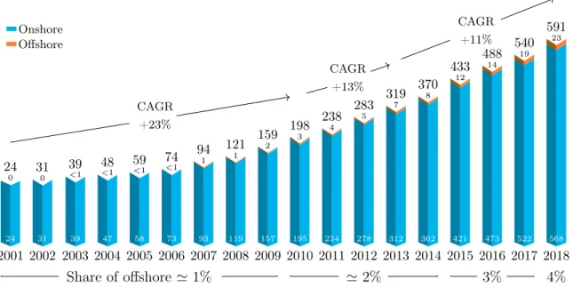
Worldwide Figure 1.5 shows that in 2018, 51.3 GW of wind electricity energy was installed. This is slightly lower than in 2017 from about 4%. Since 2014, new installations have reached 50 GW each year despite fluctuations in some markets [5]. Those new installations bring a cumulative total of installations to nearly 591 GW. For the onshore wind energy market, 46.8 GW was installed, down 4.3% compared to 2017. China and the United States remained the largest onshore markets. The global offshore market remained stable in 2018 with 4.5 GW of new installations, as in 2017. The total cumulative installations have now reached 23 GW, which represents 4% of the total cumulative installations.

For the past twenty years, there has been a slowdown in this increase, as shown in figure 1.5. Indeed, the Compound Annual Growth Rate (CAGR) (defined in equation (1.1)) goes from +23% for the period 2001-2010 to only +11% over the last six years.

(20)

1.1. GENERAL CONTEXT 19

CAGR = A2 A1

!1/N y

− 1 (1.1)

whereA2 is the final value,A1 is the initial one, andN y is the number of year in the period.

2001 24 0 24 2002 31 0 31 2003 39 <1 39 2004 47 <1 48 2005 58 <1 59 2006 73 <1 74 2007 93 1 94 2008 119 1 121 2009 157 2 159 2010 195 3 198 2011 234 4 238 2012 278 5 283 2013 312 7 319 2014 362 8 370 2015 421 12 433 2016 473 14 488 2017 522 19 540 2018 568 23 591 Share of offshore_{' 1%} _{' 2%} 3% 4% CAGR +23% CAGR +13% CAGR +11% Onshore Offshore

Detailed data sheet available in GWEC’s members only area

Figure 1.5 | Historic development of total installation in GW for the wind energy sector. Extracted from GWEC Report 2018, p27. [5]

Europe has been a leader in the development of wind energy. For instance, Denmark is produc-ing via wind power, the equivalent of 43.4% of its total electricity consumption in 2017. As shown in figure 1.6, this is the only country with the share of wind power in demand higher than 40 %. Moreover, Europe is also known for its dynamism in the development of this energy. This is the second largest region in the world in terms of growth, and there have been 11.7 GW of installations (10.1 GW in the EU) of gross electricity capacity in 2018. Figure 1.6 displays the share of wind power in demand for most European countries. It also shows the new installations (in GW) as well as cumulative installed capacity (in GW) for the five largest wind energy producing countries. We can see that Germany is the first country in terms of cumulative installed capacity with 59 GW installed and with more than 20% of wind power in demand. France is the fourth with 15 GW but with less than 10% of wind power in demand.

In any case, with a total net installed capacity of 189 GW, wind energy remains the second largest form of electricity generation capacity in Europe, even exceeding gas installations by 2019. 2018 was a record year for new wind capacity financed, and 16.7 GW of future projects are under development [5].

In France As shown in figure 1.4 wind power is the second largest renewable energy source in France (after hydroelectric). However, today, electricity production in France still relies heavily on nuclear energy. In 2018, this resource accounted for 71.7% of the electricity produced. As for

(21)

20 CHAPTER 1. INTRODUCTION 3.4 59 0.4 23 1.9 21 1.6 15 0.5 10 Share of wind power in demand 40-50% 30-40% 20-30% 10-20% 0-10% New installations in 2018 (GW) Cumulative installed capacity (GW)

Figure 1.6 | Share of wind power in total electricity demand in 2018 in Europe. The total installed capacity as well as the new installations for 2018 are shown, for the five countries with the largest installed capacity.

fossil fuels (coal, oil or gas), there has been a real drop in production. In 2018 they accounted for 7% of electricity production in France. Faced with this decline, renewable energies are devel-oping considerably, in particular hydroelectric, which produced 12.4% of electricity in 2018. This corresponds to an increase of 25% compared to the previous year, according to RTE (Réseau de Transport d’Électricité), the manager of the public electricity transmission network in France [4]. Wind and solar energies are not to be outdone. They now represent 5.1% and 1.9% of the mix with increases of 15.3% and 11.3%, respectively. Finally, bioenergy is gradually gaining ground. They accounted for 1.8% of production in 2018 [4].

The size and the geographical position of its territory give France the second largest wind energy potential in Europe after Great Britain. The Environment and Energy Control Agency (ADEME for Agence De l’Environnement et de la Maîtrise de l’Énergie) provides a map of the French wind farms: the regularly and strongly windy land areas are located on the western side of the country; it also gives an estimate of the French offshore wind potential: 30000 MWA [6].

Also, France has set ambitious renewable energy development targets in the Energy Transition Law for Green Growth, adopted in August 2015 with 15000 MW in 2018 (15117 MW recorded at the end of 2018) and between 21800 MW and 26000 MW in 2023. Moreover, this law sets France’s

(22)

1.2. STATE OF THE ART IN SHORT TERM FORECASTING 21

production of renewable energy at 40% by 2030. Thus wind energy will see its share in the French electricity mix increase each year.

To ensure that this development takes place in a favorable context, the French government introduced an incentive measure in 2000 and until 2015: the purchase obligation.

In the context of these contracts, EDF or local distribution companies purchase the wind electricity from operators who request it, at a feed-in tariff set by decree.

Under 2008 conditions, contracts for onshore wind power were signed for 15 years. The rate was set in 2008 at 8.2 cts_{¤/kWh for 10 years, then between 2.8 and 8.2 cts¤/kWh for 5 years} depending on the sites. This tariff is updated each year.

From January 1, 2016, the support for onshore wind power has evolved towards the new re-muneration system set up by the Law on Energy Transition for Green Growth. They state that the electricity produced should be sold directly by the producer on the electricity market. The difference between a reference tariff fixed by order and the average market price recorded each month is paid to the producer by EDF. The additional cost incurred by EDF is offset against a contribution called Contribution au Service Public de l’Électricité (CSPE).

In both cases, this period during which the wind producer can sell its electricity at a preferential price lasts only 15 years. At the end of this period, the producer has to sell its electricity on the competitive market. In several ways, this change can cause a significant loss of income.

On this market, electricity is sold the day before at midday for each time slot of the next day (requiring a forecast from +12 h to +35 h). A second market opens at 3 PM the day before. This market is a balancing market. Thus, having access to a more reliable forecast (because shorter term), the producer can correct his sale by buying or selling on this balancing market up to 30 minutes before the delivery date.

However, at any time, the amount of electricity fed into the grid must be equal to the quantity of electricity withdrawn. The balance between production and consumption is ensured in real time by RTE. Thus if the difference contributed to the French total deviation, it will result in a financial penalty for the producer. On the other hand, if the difference has decrease the total French deviation, the producer will receive financial compensation from RTE. However, this financial compensation is, on average, less than what the producer would have received if he could have sold this electricity on the balancing market.

Thus, having access to a reliable short term forecast to limit these gap compensations is essential for the producer. It allows to limit the loss of income due to the end of the feed-in tariffs.

1.2 State of the art in short term forecasting

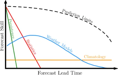
Many methods are available for wind energy forecasting. They can be classified according to time scales or methodology. The time scale classification of wind energy forecasting methods is quite arbitrary, and differs according to the different descriptions found in the literature. However, in general, four categories can be identified: the very short term, the short term, the medium term, and the long term. For the classification according to methodology, the different studies agree and each of this methodology is generally associated with a specific time scale. Figure 1.7 illustrates this classification.

It shows the performance of the different wind speed forecasting methods depending on the targeted lead time. We can see that persistence approach and statistical methods are preferred for the very short term and short term forecasting while weather models can be used for longer lead times. Finally, climatology remains the best approach for studies ranging from decades to

(23)

Figure 1.7 | Diagram of the performance of the different wind speed forecasting methods according to time.

centuries. Tables 1.1 sum up and describe these classifications with the approximate range and associated examples. Table 1.1a displays the time classification. For each category, it includes the associated range and the application of the corresponding forecasting methods. Table 1.1b displays the classification according to the methodology. Again, it shows few examples and the typical range for each category. Of course, each category remains indicative, and some models classified as short term, can be used for medium or long term forecasting.

Long term and medium term forecasts Most of the time, long term and medium term forecasts use the same techniques, which are physical models. Physical models are based on the mathematical equations that govern the physics law of the atmosphere. They are generally run on a global or regional space scale and provide, on a coarse grid, forecasts of several physical variables such as temperature, pressure, wind speed, or humidity for example. Usually, models are run once or twice a day due to the difficulty of obtaining information in a short period of time and the high cost involved. That is why they are preferred for long term or medium term forecast. For instance, in [7], Hong evaluates the NCAR (National Center for Atmospheric Research) Mesoscale Model (MM5) on a horizontal grid at a 5 km resolution. The model was run twice a day, and the study focuses on the Taïwan area within a period of two months. He focuses on surface variables and shows that the model tends to overestimate the surface wind speed. In [8], Taylor et al. use Weather Ensemble Prediction to predict the wind speed at five wind farms located across UK up to ten days ahead. Instead of producing a single forecast of the most likely weather, a whole set of forecasts is produced. This ensemble is then intended to provide an indication of the range of possible future states of the atmosphere. If statistical models are traditionally categorized for short term forecasts, they can be combined with physical methods. These hybrid methods are then used for all horizons. For instance, in [9], Salcedo-Sanz et al. hybridize the MM5 model mentioned above, with an Artificial Neural Network (ANN) to forecast the wind speed two days ahead at a wind farm located in the Southeast of Spain. The outputs of the NWP model are processed by the ANN.

(24)

1.2. STATE OF THE ART IN SHORT TERM FORECASTING 23

(a) Classification based on time scale

Category Range Example of applications

Very short term Few seconds to - Electricity market clearing few tens of minutes - Real time grid operations

Short term Few tens of minutes - Economic load dispatch planning to few hours

Medium term Several hours to - Generator online/offline decisions to few days - Unit commitment decisions Long term Few days to - Maintenance planning

one year (or more) - Feasibility study for design of the wind farm (b) Classification based on methodology

Methodology Examples Range

Persistence method / Very short and

short term Statistical approaches - Artificial Neural Network (ANN) Short term

- Time series based models

Physical approach - Numerical Weather Prediction (NWP) models Medium and long term

Hybrid methods

- NWP + ANN

All ranges - Spatial correlation + ANN

- NWP + time serie based model

Table 1.1 | Classification based on time scale (table 1.1a) and on methodology (table 1.1b) for the wind energy forecasting. In table (a), an approximate range and two examples of applications are shown for each category. In table (b), for each methodology, the associated typical range and few examples are shown.

Very short term forecasts Very short term forecasting is the least represented category in the literature. Typically these forecasts range from few seconds to several minutes and are almost exclusively provided by statistical methods such as time series based model or ANN. For such lead times, they are never combined with NWP models and only use historical in-situ data as input. In [10], Riahy et al. use a time series based method to predict the wind speed 1 sec to 5 sec ahead for control system of wind turbines such as changing the pitch angle of the blades. In [11], Potter et al. use a model based on neural networks to forecast wind vectors up to 2.5 min ahead in Tasmania, Australia.

Short term forecasts Short term forecasting is the main objective of this thesis. As shown in table 1.1a, short term forecasts usually range from tens of minutes to a few hours. Short term forecasts 1 h ahead are the most studied forecasts in the literature. In this thesis, we will focus on forecasts from 10 min to 3 h ahead.

As shown in table 1.1b, for these time scales statistical methods are the most used. They may or may not be combined with physical methods as in [9]. Statistical approaches aim at finding the relationship between past and future observations. Historical data are used as input, and in the case of hybrid methods, NWP model outputs are also added.

Statistical methods can be divided into two sub-categories: those based on linear time series that are easy to model and inexpensive to implement, and those based on artificial intelligence

(25)

methods. These can treat non-linearity but are more complicated to set up and are known to be black-box models. Most of the time, these models are tested against the persistence model, which is the benchmark approach for this time scale. Persistence assumes that wind speed or wind energy at timet = t0+ ∆t will be the same as at time t0.

In [12], Chang uses a back propagation neural network, which consists of feeding the network backward during the training period to tune the parameter more accurately. His goal is the wind power forecasting 10 min ahead. For the best NN, he finds a maximum absolute error of 2.0% and an average absolute error of 0.3%. In [13], Kariniotakis et al. develop a NN for wind power time series forecasting up to 2 h ahead. They compare 3 differents NN. Among the 3 models, the one that performs best for the first lead times is also the one that performs worst for the longer lead times and vice versa. For the third model, they find an improvement over persistence around 10%, for the whole period. In [14], Zhao et al. investigate a hybrid wind forecasting method. It consists of a NN fed with NWP model outputs. Their goal is the wind power forecasting 1 h ahead at a specific wind farm in China. They find that the Normalized Root Mean Square Error (NRMSE) has a monthly average value of 16.47% which they give as an acceptable value to guide the penetration of wind energy in China.

In [15], Palomares-Salas et al. develop a time series based model (ARIMA) used to predict the wind speed. The results are compared with the performance of a back propagation NN. They show that the ARIMA model overperforms the NN model for the short term lead times (10 min, 1 h, 2 h, and 4 h). In [16], Panteri et al. also compare NN and time series based model for wind power forecasting at three different wind farms for look-ahead times between 1 h and 12 h. They use a simple configuration for the time series based method (ARX), and they find that this model cannot overperform persistence for the whole period. However, NN is better than the persistence model. In [17], Firat et al. develop a model to forecast the hourly wind speed. Their starting point is the time series based model AR. Their implementation of this model leads to an improvement over persistence for the whole period. Moreover, the traditional AR is the model that shows the best improvement for the first lead time (1 h).

While neural network and time series based methods remain the most commonly used and the most studied models for wind speed and wind energy short term forecasting, many other methods have been investigated. For instance, in [18], Alexiadis et al. implements a NN based on spatial correlation to forecast the wind speed at six different sites, on islands of the South and Central Aegean Sea in Greece, distant from 52 km to 105 km. Their goal is the wind speed forecasting for the next 1 h, 2 h, and 3 h. The model is tested using data collected over seven years, and its performance are considered satisfactory. In [19], Pinto et al. propose a Support Vector Machines (SVM) model for short term wind speed forecasting. Its performance is evaluated and compared with ANN based approaches. SVM models are non-parametric models for classification and regression problems, such as pattern recognition or regression analysis. A case study for predicting wind speed at 5 min intervals is presented. Results show that the best parametrization for the proposed SVM achieves better forecasting results than the ANN based approaches. In [20], Lahouar et al. propose a random forest method to build a 1 h ahead wind power forecasting system. Like SVM, random forests are non-parametric models designed for classification and regression problems. The algorithm builds decision trees and performs learning on multiple trees trained on slightly different subsets of data. Results show an improvement of forecast accuracy using the proposed model, as well as an important reduction of the different error criteria compared to classical NN prediction. Finally, in [21], Castellanos et al. use a ANFIS model to forecast the hourly wind speed. The Adaptive Neuro-Fuzzy Inference Systems (ANFIS) is a hybrid model between ANN and Fuzzy Inference Systems (FIS). If the ANN part can search for patterns, which gives the

(26)

1.3. THESIS OBJECTIVES AND CONTEXT 25

advantage of learning about systems, the FIS part is based on fuzzy logic. It corresponds to a set of fuzzy IF–THEN rules that learns capability to approximate nonlinear functions. Generally, this type of model shows more promising results than a single ANN. In [21], they obtain errors between 25.5% and 32.5% depending on the configuration.

1.3 Thesis objectives and context

The general issue raised in this work is to know if an accurate short term forecasting model can ensure the penetration of wind energy in the electricity grid and if it can compensate for the decrease in income due to the end of the feed-in tariffs period. Only few studies have been done for 30-min ahead, which is the deadline for balancing on the electricity market. In addition, the model must be efficient for these short lead times but also for longer lead times since the balancing market opens several hours before the delivery date. In this context, several questions can be raised:

1. How can the state of the art on wind energy forecasting can be improved for time horizons from few tens of minutes to few hours?

2. What is gained by including available ancillary measurements as input, such as wind direction, wind variability, or temperature?

3. Can wind energy production data from multiple wind farms improve the forecast at a given wind farm?

4. What is the economic value of short term forecasts for a wind energy producer?

This study will be carried out based on the case of a French wind energy producer. Indeed, this work is supported by a private company called Zephyr ENR1_{. The company, created in 2002,}

is the result of a partnership between an agricultural advisory office in France and a wind power development office in Germany. More precisely, Zephyr ENR is a wind farm development and operation office whose objective is the emergence of participatory projects in which farmers, local residents, and rural people are partners in the development and ownership of wind turbines. Since 2002, six wind farms have been built in France, including 31 wind turbines representing 77 MW and 130000 MWh/year. These wind farms are distributed in the northwest quarter of France and grouped by two, as shown in figure 1.8. Parc de Bonneval (A), Parc de la Renardière (B), and Parc de Beaumont (C) are composed of six 2 MW turbines. Moulin de Pierre (E) is composed of six 3 MW turbines. Parc de la Haute Chèvre (D) is composed of three 2.3 MW turbines and Parc de la Vènerie is composed of four 2.3 MW turbines. For each wind turbine, a substantial amount of data is recorded and transmitted at a frequency of 10 min. We can mention the wind speed, the wind direction, the production, the temperature, and the pitch angle, for example. The first farm has been in service since 2006.

Consequently, in 2021, the feed-in tariffs period will end for this farm, and the company will have to sell its energy on the competitive market.

1.4 Thesis outline

First of all, in chapter 2, a short term wind speed forecasting model is proposed. This model is a hybrid model based on the statistical parametric downscaling of NWP model outputs and

1

(27)

Figure 1.8 | Location of the wind farms owned by Zephyr ENR. There are Parc de Bonneval (A), Parc de la Renardière (B), Parc de Beaumont (C), Parc de la Haute Chèvre (D), Moulin de Pierre (E), and Parc de la Vènerie (F) .

on time series based model. Its performance is compared with the benchmark model, such as the persistence approach, ARMA method, and NN. A non-parametric approach is also used for comparison with a random forest method. The proposed model is evaluated for hourly forecasts from 1 h to 11 h ahead and forecasts at 10 min frequency from 10 min to 3 h ahead.

Then, in chapter 3, the conversion from wind speed forecasts to wind power forecasts is op-timized. Using the data collected at the wind turbines, the influence of wind direction and air density on the power output is quantified. Methods to take into account these features are de-scribed and evaluated. A sensitivity study on the impact of atmospheric conditions such as wind shear, turbulence, or atmospheric stability is also conducted.

In chapter 4, the fact that the wind farms are grouped by two is tapped. Models based on spatial correlation are explored. The added value of small scale information is first evaluated using two adjacent farms. A few kilometers away, this configuration is adapted for the first lead times that we are interested in, typically from 10 min to 30 min. Then, the impact of large scale information is investigated using data from distant farms. This time, the configuration is more likely to perform well for the longest lead times (>1 h). In both cases, regimes based on the wind direction are distinguished.

Finally, the goal of chapter 5 is to quantify the economic value of a short term forecasting model for a producer. Simulations are performed using in-situ data and data from the actual electricity market. The case where no short term forecasts are available, and the case where a short term forecasting model is used are analyzed, and the different sources of variability are highlighted.

(28)

2 Sub-hourly forecasting

of wind speed

Contents 2.1 Introduction . . . 28 2.2 Methodology . . . 29 2.2.1 Parametric downscaling approaches . . . 29 2.2.2 Non parametric downscaling approaches . . . 31 2.2.3 Benchmark methods . . . 32 2.3 Application at two wind farms . . . 36 2.3.1 Performances for hourly forecasts . . . 37 2.3.2 Performances for sub-hourly forecasts . . . 41 2.4 Analysis of the best model . . . 45 2.5 Conclusion . . . 47

(29)

2.1 Introduction

The intermittency of wind is the main barrier to the development of wind energy. For this resource to establish itself as one of the primary renewable resources on a sustainable basis, it is necessary to allow its penetration on a large scale. However, many difficulties must be overcome to ensure the stability of the system, such as grid operation management, maintenance scheduling, electricity market clearing, for example. Improving wind forecasting is one way to achieve higher penetration of wind power in the electricity system. In the context of climate change and energy transition, this issue is becoming a priority, and over the past two decades, the global energy market is turning increasingly to green energies.

Fortunately, Numerical Weather Prediction (NWP) models have improved significantly over the last 30 years. The forecast skill of the 3-days forecasts for the northern hemisphere rose from 85% to 98.5% between 1981 and 2013 and from 70% to 98.5% for the southern hemisphere [22]. The poor performances in the southern hemisphere was due to a lack of measurement in the region. Even though NWP models perform well for predicting large scale meteorological variables at short term, like mid-tropospheric pressure, they do not perform the same for variables having high variability at small scales, like surface winds. Large scale variables are well understood physically and efficiently modeled numerically, but the variables tied to phenomena occurring on a smaller scale depend more on processes that are not resolved and so parametrized. This leads to significant model errors for variables like surface wind.

The model error has several components: part comes from the inadequate representation of physical processes, e.g., uncertainties in the parametrizations used for boundary layer turbulence. Improving parametrizations should reduce this error. Part of the error is numerical error, coming from the discrete representation of a continuous process. Also tied to the limited resolution is the representativity error, which occurs because of the difference of the value over a grid box and the value at a specific point. Downscaling methods such as Model Output Statistics (MOS) are usually used to reduce representativity error [23]. Those models have been developed in the weather forecast for several decades based on NWP model outputs. A statistical relationship is determined between observations and forecasts using past forecasts and corresponding observations and then serves to improve predictions at that observation site.

Downscaling models can be very interesting to get accurate forecasts at a specific location of a wind farm [24]. To do so, different downscaling models and different outputs of NWP models, climate data, or, if relevant, recent surface observations can be used as explanatory variables for the near surface wind speed [25]. Amongst them, markers of large-scale systems (geopotential, pressure fields) and boundary layer stability drivers (surface temperature, boundary layer height, wind, and temperature gradient) can be used [26]. In terms of methodology, several models have already been studied, including linear regression, Support Vector Machine (SVM), or random forests.

However, for hourly and sub-hourly forecasts, downscaling methods are not commonly used because NWP models are only run once or twice a day due to the difficulty of gaining information in a short time and the associated high costs. This usually limits its usefulness to forecasts with lead times longer than 6 hours, at least. Persistence is the reference method for short term and very short term forecasts. It supposes that the wind speed at a particular future time will be the same as it is when the forecast is made. It is extremely accurate for a very short lead time, but its performance degrades rapidly with time. Statistical approaches are also used as a benchmark for short and very short term generally. We can split this category into two sub-categories, which are artificial intelligence methods such as Artificial Neural Network (ANN) using past measure-ments as explanatory variables and time series models such as Auto-Regressive Moving Average

(30)

(ARMA) [27]. ANN models can represent a complex non-linear relationship and extract the depen-dences between variables through the training process. Statistical methods are based on training with measurements and use differences between the predicted and the actual wind speed to up-grade the model. Both approaches constitute the reference methods for short term forecasts [28]. Usually, ANN models outperform time series models [29] even if some very good time series models can supersede ANN methods [30, 31].

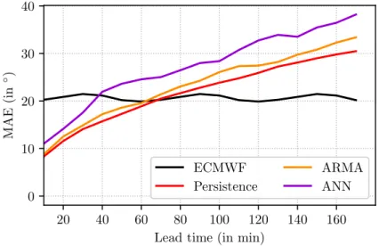
In this chapter, we compare two configurations of downscaling models tested on several wind farms. The first configuration uses explanatory variables available from NWP models, and the second one adds explanatory variables derived from observations. In both cases, we compare the results of linear regression and random forests with persistence methods and with the benchmark methods. The chapter is organized into five sections. The next section describes the data and the different models. In section 2.3, results are analyzed. As there is little literature on sub-hourly time scales, we first (2.3.1) test our methods on hourly time scales, from 1 h to 11 h, which are much more documented. Results of persistence, ARMA, and ANN methods are also shown for comparison with the classical results found in the literature. Then, all methods are applied for sub-hourly forecasts from 10 min to 170 min at a frequency of 10 min (2.3.2). In section 2.4, the best model is analyzed in more detail. In the last section, we discuss the results and conclude.

2.2 Methodology

2.2.1 Parametric downscaling approaches

Downscaling statistical methods have been widely investigated since several decades in order to forecast the wind speed, usually from few to several hours [32, 33, 34]. In this thesis we consider linear regression, a very easy to implement method and numerically low cost [35]. The parametric approach supposes a relation between the target at timet, ybt and the m explanatory variables at timet, X1,t, ..., Xm,t: b yt= ω0+ m X k=1 ωkXk,t+ ε (2.1)

whereωi,i∈ {0, ..., m}, are the model parameters to be estimated by a classical Ordinary Least

Squares (OLS) method andε is the residual following a centered normal distributionN (0, σ2_{). The}

explanatory variables are chosen among ECMWF (European Centre for Medium-Range Weather Forecasts) outputs. It provides global forecasts, climate reanalyses, and specific datasets.In our case, we retrieve the day-ahead hourly forecasts, starting from analysis twice a day, at 00:00 UTC and 12:00 UTC. UTC is the Universal Time Coordinate. However, we would like the downscaling models to be able to start at any time and not only twice a day. In these conditions, we need to dissociate the lead times from ECMWF and the lead times from the downscaling models. For instance, the first lead time t0+ 1 h for the dowscaling models may not be the first lead time for

ECMWF. If a forecast from the downscaling models is launched at 05:00 UTC, the first lead time is 06:00 UTC. However, this is the sixth lead time t0+ 6 h for ECMWF as the forecast started

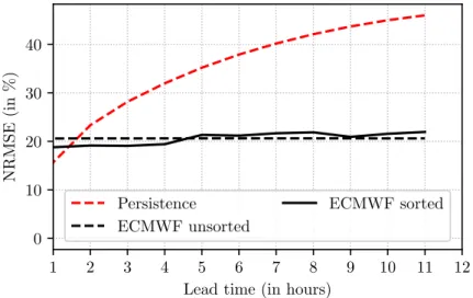
at 00:00 UTC. To be sure that this mixing of lead times does not introduce significant errors into the downscaling model, we investigate whether the ECMWF error over the first 12 hours increases significantly or not. Figure 2.1 displays the forecasted error of ECMWF in % (defined later in equation (2.8)) along with persistence (described in 2.2.3). It shows that for the first 12 hours, whether the forecasts start at 00:00 UTC or at 12:00 UTC (’ECMWF sorted’) or if the forecast

(31)

starts at any time (’ECMWF unsorted’) the errors are close. Then hereafter, t0 does not refer to

00:00 UTC or 12:00 UTC, but it refers to the time when the downscaling models are launched.

1 2 3 4 5 6 7 8 9 10 11 12

Lead time (in hours) 0 10 20 30 40 NRMSE (in %)

Sizing of a Short-Term Wind Energy Forecasting System – Manuscript – Chapter. 2

Persistence ECMWF unsorted

ECMWF sorted

Figure 2.1 | Comparison of ECMWF performances whent0refers to 00:00 UTC or 12:00 UTC

(’ECMWF sorted’) and when t0 refers to the starting time of the downscaling models

fore-casts (’ECMWF unsorted’). In the first case, there are two forefore-casts a day (00:00 UTC or 12:00 UTC), in the second cases these are hourly forecasts. The performance of persistence (described in 2.2.3) is added as reference.

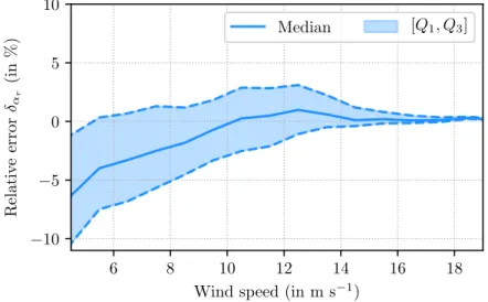
The downscaling model is trained using 47 variables aiming at describing the boundary layer, winds and temperature in the lower troposphere. Tables 2.1, 2.2 and 2.3 show the considered variables. The large scale circulation brings the flow to the given location. The wind speed in altitude, the geopotential height, the vorticity, the flow divergence, or the temperature can be markers of large systems like depressions, fronts, storms, or high pressure systems (table 2.2). At a finer scale, what is happening in the boundary layer is very important to explain the intra-day variations of the wind speed. The state and stability of the boundary layer can be derived from surface variables describing the exchanges inside the layer. Exchanges are driven mostly by temperature gradient and wind shear that develop turbulent flow (table 2.3). Thermodynamical variables like surface, skin, and dew point temperatures and surface heat fluxes can also inform on the stability of the boundary layer, as well as its height and dissipation on its state (table 2.1). The spatial resolution of ECMWF forecasts is of about 16 km (0.125◦ in latitude and longitude).

Among the explanatory variables,X1,t, ..., Xm,t, some provide more important information, and

some may be correlated. Thus, a stepwise regression (forward selection) is performed to only keep the most important uncorrelated variables [35]. This is an iterative regression, which consists of adding variables from the set of explanatory variables based on the Bayesian Inference Criterion (BIC) [36]. The BIC is based on the likelihood function, and it reduces overfitting by introducing a penalty term for the number of parameter in the model. The model with the lowest BIC is preferred. At each step, a model is built by adding one variable among the remaining ones. The added variable which minimizes the BIC of the model is chosen. The procedure is repeated as long as the BIC decreases.

The linear regression considering all the explanatory variables given in tables 2.1, 2.2 and 2.3 is denoted LR_A and the linear regression considering a sample of explanatory variables (selected

(32)

Altitude (m) Variable Unit Name

10 m / 100 m Zonal wind speed m s−1 u

Meridional wind speed m s−1 v

2 m Temperature K t

Dew point temperature K dp

Surface

Skin temperature K skt

Mean sea level pressure Pa msl

Surface pressure Pa sp

Surface latent heat flux J m−2 slhf Surface sensible heat flux J m−2 sshf - Boundary layer dissipation J m−2 bld

Boundary layer height m blh

Table 2.1 | Surface variables

Pressure level (hPa) Variable Unit Name

1000 hPa / 925 hPa / 850 hPa / 700 hPa /

500 hPa

Zonal wind speed m s−1 u Meridional wind speed m s−1 v Geopotential m2 s−2 z

Divergence s−1 d

Vorticity s−1 vo

Temperature K t

Table 2.2 | Altitude variables

Altitude Variable Unit Name

10 m / 100 m Norm of the wind speed m s−1 F

10 m to 925 hPa Wind shear m s−1 DF

2 m to 925 hPa Temperature gradient K DT

Table 2.3 | Computed variables

by the stepwise regression) is denoted LRSW.

2.2.2 Non parametric downscaling approaches

Non-parametric models do not suppose to advance a specific relation between the variables. In-stead, they try to learn this complex link directly from the data itself. As such, they are very flexible. The family of non parametric is quite large. Among others, one may cite the nearest neighbor’s rule, the neural network, support vector machines, regression trees, random forests, for example. Regression trees which have the advantage of being easily interpretable, show to be particularly effective when associated with a procedure allowing to reduce their variance as for Random Forest Algorithm. Regression trees are binary trees built by choosing at each step the cut minimizing the intra-node variance, over all explanatory variables X1,t, ..., Xm,t, and all possible

(33)

D(Xk, Sk) = X Xk<Sk (ys− ¯y−)2+ X Xk≥Sk (ys− ¯y+)2 (2.2)

where y¯− (respectively y¯+_{) denotes the averaged of the target in the area} _{X

k < Sk}

(re-spectively _{X_k _{≥ S}_k_{}). Then, the selected k}₀ variable and associated threshold is given by (Xk0, Sk0) = arg min

(k,Sk)

D(Xk, Sk). The prediction is provided by the value associated to the leaf in

which the observations falls.

To reduce variance and avoid over-fitting, it is interesting to generate several bootstrap samples, then fit a tree on every sample and average the predictions, which leads to the so-called Bagging procedure [37]. More precisely, forB bootstrap samples, the predicted value is given by:

ˆ y = 1 B B X b=1 ˆ yb (2.3)

whereyˆb_{is the value predicted by the regression tree associated with the}_b_{−th bootstrap sample.}

To produce more diversity in the trees to be averaged, an additional random step is introduced in the previous procedure leading to Random Forests. In this case, the best cut is chosen among a smaller subset (corresponding to 1

3m variables, where m is the total number of explanatory variable) of randomly chosen variables. The predicted value is the mean of the predictions of the trees, as in equation (2.3). Hereafter, this model is denoted RF. Again, the explanatory variables are retrieved from ECMWF forecasts and given in tables 2.1, 2.2 and 2.3.

Each model introduced above: LR_A, LR_SW, and RF has been tested using in-situ measurements collected at three wind farms called Parc de Bonneval, Moulin de Pierre and Parc de la Vènerie. For the three models, two configurations are tested. The first one consists of a classical downscaling using the explanatory variables available from ECMWF outputs only. The second one consists of adding the error between the observed wind speed at time t0, i.e., when the forecast is launched,

and the forecasted wind by ECMWF at time t as an explanatory variable. Hereafter, when the models are trained according to the first configuration, they are denoted LRno-obs_A , LRno-obs_SW , and

RFno-obs. When the models are trained according to the second configuration, they are denoted

LRobs

A , LRobsSW, and RFobs.

In the first case, only one model is fitted. In the second case, a model is fitted at each hour in order to precisely take into account the error between the forecasted wind at time t and the observations at timet0. For the second configuration, after the variable selection step, between 14

and 21 variables remain, depending on the horizon. In [35], Alonzo et al. compare this low cost assimilation to the downscaling without in-situ information. For a 3 h lead-time, they can improve the forecast up to 18% by considering the initial error.

2.2.3 Benchmark methods

For short term predictions, statistical methods are the most used and are always compared to persistence [27]. Persistence assumes that the wind speed at time t will be the same as it was at time t0. Although this model is very simple, it is, in fact, difficult to beat for look-ahead times

from 0 to 4-6 hours. This is due to the fact that changes in the atmosphere take place rather slowly [17]. The statistical approach aims at finding the relationship between past and future observations using measurements (and possibly exogenous variables). They can be split into two

(34)

sub-categories: time series based models which are easy to model and cheap to develop an artificial neural network which can deal with non-linearity but which is known as black box model.

Time series models are mainly based on Auto-Regressive Moving Averaged (ARMA) models [38]. An ARMA(p, q) model aims at predicting the wind speed at time t, using a linear combination of thep previous wind speed values, the q previous residuals and potentially m exogenous variables (in that case we define the model as ARMAX). The most sophisticated models are ARIMAX(p, d, q) for Auto-Regressive Integrated Moving Averaged EXogenous. They aim at removing the non-stationarity of the data by applying an initiald-order differencing step as follow:

b yt= p X i=1 Φi∆dyt−i+ q X j=1 θjεt−j + m X k=1 βkXk,t (2.4) ∆dyt= (yt− yt−1)− d−1 X i=1 (y_t−i_{− y}_t−(i+1)), d = 1, ..., n (2.5)

wherey_t−i is the observed wind speed at timet_{− i, Φ}i, θj, βk are the model parameters,∆d is

thed-order lag operator defined in equation (2.5), εt−j is the residual at timet− j, and Xk,t is the

kth _{explanatory variable at time}_{t, which can be an output from NWP.}

Artificial neural networks (ANN) are models inspired by biological neural networks. They are based on interconnected groups of nodes, divided into layers. Each connection can transmit a signal from one artificial neuron to another. An artificial neuron that receives a signal can process it and transmit it to another neuron. Usually, this signal is a set of real number, and the output of each artificial neuron is computed by some non-linear function, called activation function, of a weighted sum of its input. The weights and the activation function are updated through the training process [39, 40]. Those models are very useful in the modeling of complex non-linear relationships and extract dependences between variables.

Choice of the parameters

The choice of the benchmark model parameters is a crucial step. For both hourly and sub-hourly forecasts, we fit several models, and we choose the most efficient one. For the ARMA models, we use the BIC to select the models. For several values of the p and q parameters, we fit the corresponding models, and the model that minimizes the criterion is preferred. Figure 2.2 displays the results for hourly forecasts (a) and sub-hourly forecasts (b) at Parc de Bonneval. For the first one, an ARMA(6,3) appears to be the best model, and for sub-hourly forecasts, it is an ARMA(4,2). The same procedure is applied for Parc de la Vènerie and Moulin de Pierre. At Moulin de Pierre (resp. Parc de la Vènerie), an ARMA(5,3) (resp. ARMA(2,1)) gives the best results for the hourly forecasts. For the sub-hourly forecasts, the selected model is at Moulin de Pierre (resp. Parc de la Vènerie) is an ARMA (3,3) (resp. ARMA(5,4)).

For the ANN, we compute the RMSE, defined in equation (2.6), as a function of the number of layers and the number of neurons per hidden layer. Results are shown for the first lead time. We fix the seed in order to better compare the model’s performance and remove the noise due to the stochastic nature of ANN.

RMSE= v u u t 1 N N X i=1 (y_bi− yi)2 (2.6)

(35)

Figure 2.2 | Bayesian Inference Criterion (BIC) of different ARMA(p,q) models depending on the AR order p and the MA order q for the hourly forecasts (a) and the sub-hourly forecasts (b) at Parc de Bonneval.

In equation (2.6),_byi is thei-th wind forecast and yi is the corresponding observation. N refers

to the number of forecasts that have been done to compute the RMSE.

According to figure 2.3, at Parc de Bonneval, the best ANN for the hourly forecasts is a model with 2 layers (one hidden layer and one output layer) with 10 neurons in the hidden layer and the best model for sub-hourly forecasts is an ANN with 4 layers and 10 neurons in the hidden layers. Again, the same procedure is applied for Parc de la Vènerie and Moulin de Pierre. At Moulin de Pierre the same configuration than at Parc de Bonneval is used for the hourly forecasts, and at Parc de la Vènerie, an ANN with 2 layers and 40 neurons in the hidden layer is chosen. For sub-hourly forecasts an ANN with 4 layers and 30 neurons in the hidden layers is chosen at Moulin de Pierre and an ANN with 4 layers and 10 neurons in the hidden layers is chosen at Parc de la Vènerie.

10 20 30 40 50 Number of nodes per hidden layer

1 2 3 4 5 Num b er of la yers

(a) Hourly forecasts

0.98 0.99 1.00

RMSE

10 20 30 40 50 Number of nodes per hidden layer

1 2 3 4 5 Num b er of la yers (b) Sub-hourly forecasts 0.495 0.500 0.505 RMSE

Figure 2.3 | RMSE for the first lead time of different ANN model depending on the number of hidden layers and the number of neurons per hidden layer. The results for hourly forecasts (a) and sub-hourly forecasts (b) are shown.

(36)

Use of exogenous variables

Both ARMA and ANN can be used as pure time-series based models or with exogenous variables. Figure 2.4 displays the comparison of the error distributions at Parc de Bonneval for the forecasts at t0+ 1 h and t0 + 3 h between ARMA and ARMAX and between ANN and ANNX. We use

only the 100 m wind speed (F =√u2_{+ v}2_{) forecasted by ECMWF as exogenous variable. For a}

lead time of 1 h, the distributions between the pure time-series based models and the models with exogenous variable do not differ significantly. For both ARMA and ANN, the interquartile range (IQR) is slightly reduced by the use of exogenous variables. From 1.63 m s−1 to 1.42 m s−1 for ARMA and from 1.10 m s−1to 1.07 m s−1for ANN. However, it slightly degrades the bias as it goes from -0.02 for ARMA to -0.03 for ARMAX and from -0.16 for ANN to -0.22 for ANNX. For a lead time of 3 h, the results are the same with a more significant gain. The IQR is reduced from 2.25 for ARMA to 1.71 for ARMAX and from 2.09 for ANN to 1.43 for ANNX. The scope, defined as the difference between the highest and lowest value, is also significantly reduced compared to the lead time of 1 h. Att0+1 h, the differences start to be visible. However, our goal is sub-hourly forecasts

with lead times starting from 10 min. At those time scales, the hourly exogenous variables carry less information than in-situ measurements. Under these conditions, we keep a pure time-series based approach for ARMA and ANN.

Figure 2.4 | Comparison for Parc de Bonneval between the pure time-series based ARMA (resp. ANN) and a model with the 100 m wind speed forecasted by ECMWF as exogenous variable ARMAX (resp. ANNX). The distribution of the error between the forecasted wind speed (using ARMA, ARMAX, ANN and ANNX) and the measurements are shown att0+ 1 h

andt0+ 3 h.

Data standardization

For both ARMA and ANN, the dataset has to be standardized so as to tend a distribution, close to a Weibull distribution (see 2.5), towards a standardized Gaussian distribution. This transformation allows ARMA and ANN to give optimal results. The standardized dataset is easily obtained by centering and reducing the data, as shown in equation (2.7).