Computational and statistical challenges in high dimensional statistical models

(1)

Computational and statistical challenges

in high dimensional statistical models

by

Ilias Zadik

B.A., National Kapodistrean University of Athens (2013)

M.A.St., University of Cambridge (2014)

Submitted to the Sloan School of Management

in partial fulfillment of the requirements for the degree of

Doctor of Philosophy in Operations Research

at the

MASSACHUSETTS INSTITUTE OF TECHNOLOGY

September 2019

c

○ Massachusetts Institute of Technology 2019. All rights reserved.

Author . . . .

Sloan School of Management

July 6, 2019

Certified by . . . .

David Gamarnik

Professor of Operations Research

Thesis Supervisor

Accepted by . . . .

Patrick Jaillet

Dugald C. Jackson Professor

Co-Director, Operations Research Center

(2)

(3)

Computational and statistical challenges

in high dimensional statistical models

by

Ilias Zadik

Submitted to the Sloan School of Management on July 6, 2019, in partial fulfillment of the

requirements for the degree of

Doctor of Philosophy in Operations Research

Abstract

This thesis focuses on two long-studied high-dimensional statistical models, namely

(1) the high-dimensional linear regression (HDLR) model, where the goal is to recover a hidden vector of coefficients from noisy linear observations, and

(2) the planted clique (PC) model, where the goal is to recover a hidden community structure from a much larger observed network.

The following results are established.

First, under assumptions, we identify the exact statistical limit of the model, that is the minimum signal strength allowing a statistically accurate inference of the hidden vector. We couple this result with an all-or-nothing information theoretic (IT) phase transition. We prove that above the statistical limit, it is IT possible to almost-perfectly recover the hidden vector, while below the statistical limit, it is IT impossible to achieve non-trivial correlation with the hidden vector.

Second, we study the computational-statistical gap of the sparse HDLR model; The statisti-cal limit of the model is significantly smaller than its apparent computational limit, which is the minimum signal strength required by known computationally-efficient methods to perform sta-tistical inference. We propose an explanation of the gap by analyzing the Overlap Gap Property (OGP) for HDLR. The OGP is known to be linked with algorithmic hardness in the theory of average-case optimization. We prove that the OGP for HDLR appears, up-to-constants, simul-taneously with the computational-statistical gap, suggesting the OGP is a fundamental source of algorithmic hardness for HDLR.

Third, we focus on noiseless HDLR. Here we do not assume sparsity, but we make a certain rationality assumption on the coefficients. In this case, we propose a polynomial-time recovery method based on the Lenstra-Lenstra-Lóvasz lattice basis reduction algorithm. We prove that the method obtains notable guarantees, as it recovers the hidden vector with using only one observation.

Finally, we study the computational-statistical gap of the PC model. Similar to HDLR, we analyze the presence of OGP for the PC model. We provide strong (first-moment) evidence

(4)

that again the OGP coincides with the model’s computational-statistical gap. For this reason, we conjecture that the OGP provides a fundamental algorithmic barrier for PC as well, and potentially in a generic sense for high-dimensional statistical tasks.

Thesis Supervisor: David Gamarnik Title: Professor of Operations Research

(5)

(6)

Acknowledgments

First and foremost, I would like to thank my advisor David Gamarnik. I was very lucky to be advised by him during the years of my PhD. During my time at MIT, I learned plenty of things and by far the most I learned from David. Beyond introducing me to numerous fascinating research questions and results across probability theory, statistical inference, statistical physics and computer science, my collaboration with David has taught me the value of optimism, patience and devotion to research. I wish that in the future I will be as good and influential an advisor to my students, as David was to me.

I would also like to thank Jennifer Chayes and Christian Borgs, who mentored me during my internship at Microsoft Research New England in the summer of 2017. In my time there, Jennifer and Christian, together with Adam Smith from Boston University, introduced me to the notion of differential privacy and its connection with network and random graphs estimation. I would like to thank all three of them for tireless long and technical discussions on the theory of privacy and random graphs, which have significantly improved my understanding on these two fascinating research topics. Many techniques and ideas used in this thesis were influenced by these discussions.

Over my PhD, I had the pleasure to collaborate on research with more people. I would like to thank all of them, I have learned something from each one of you! Specifically, I would like to thank Galen Reeves and Jiaming Xu for many conversations on the limits of sparse regression which lead to the creation of the second chapter of the present thesis, Yury Polyanskiy and Christos Thrampoulidis for exploring with me various fundamental questions on information theory, Vasilis Syrgkanis and Lester Mackey for working together on a beautiful problem on the theory of orthogonal machine learning, Juan Pablo Vielma and Miles Lubin for numerous discussions on integer programming and convex geometry and Patricio Foncea and Andrew Zheng for running certain very useful simulations for the work presented in the fifth chapter of this thesis. A big thank you also to Guy Bresler and Yury Polyanskiy for multiple mathematical discussions over these years both during their reading groups at LIDS and IDSS and while I was their teaching assistant for the graduate class "Moden Discrete Probability"; I have learned a lot from both of you. I would like to further acknowledge Guy Bresler and Lester Mackey for serving as members of my PhD thesis committee, it has been a pleasure sharing with you the

(7)

material included in the present thesis.

Doing my PhD at the Operations Research Center (ORC) at MIT has been an extremely influential experience for me. The ORC offers a unique and excellent interdisciplinary academic environment, which has broadened my perspective on mathematics and their applicability across various disciplines of science. A special acknowledgment to Dimitris Bertsimas, both for intro-ducing me to the ORC more than six year ago, when I was still an undergraduate student at the Mathematics department of the University of Athens, and for being my mentor from that point forward. Finally, I would also like to thank all the people at the ORC who make it the unique place it is!

I would also like to express my gratitude to all the professors at the Mathematics Department of the University of Athens, for showing me the beauty of mathematics over the four years that I was an undergraduate student there!

On a more personal level, I would like to dedicate the present thesis to the memory of my beloved father, Pavlos Zadik. My father passed away very suddenly during the first month of my PhD studies at MIT. His strong values on the pursuit and importance of knowledge will always provide for me a strong guidance in life. I would also like to deeply thank my mother Nelli and my sister Mary who have always been next to me; without them none of this would have been possible. Finally, I would like to thank my cousin Joseph and his lovely family for always offering a warm place in Boston when it was needed.

Last but not least, I would like to thank all the friends I have made over these years, it has been a lot of fun! A special thanks goes to my dear friends and roomates Manolis, Konstantinos and Billy for building a warm family environment, wherever we lived together over the last five years. This has been truly an amazing experience!

(8)

(9)

List of Figures

2-1 The phase transition diagram in Gaussian sparse linear regression. The 𝑦-axis is the increment of mutual information with one additional measurement. The area of blue region equals the entropy 𝐻(𝛽*₎_{∼ 𝑘 log(𝑝/𝑘). Here by 𝑛}* _{we denote the}

𝑛info. . . 44

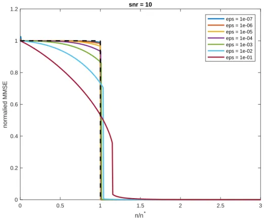
2-2 The limit of the replica-symmetric predicted MMSE _ℳ𝜀,𝛾(·) as 𝜖 → 0 for signal

to noise ratio (snr)𝛾 equal to 2. Here by 𝑛* _{we denote the} _𝑛

info. . . 47

2-3 The limit of the replica-symmetric predicted MMSE _ℳ_𝜀,𝛾(_{·) as 𝜖 → 0 for signal} to noise ratio (snr)𝛾 equal to 10. Here by 𝑛* we denote the𝑛info. . . 48

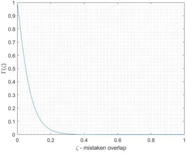
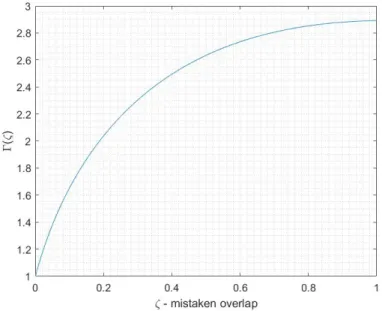
3-1 The first two different phases of the function Γ as 𝑛 grows, where 𝑛 < 𝑛info. We

consider the case when 𝑝 = 109_{, 𝑘 = 10 and 𝜎}2 _{= 1. In this case} _⌈𝜎2_{log 𝑝}_{⌉ =}

21,⌈𝑛info⌉ = 137 and ⌈(2𝑘 + 𝜎2) log 𝑝⌉ = 435. . . 109

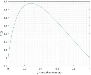
3-2 The middle two different phases of the function Γ as 𝑛 grows where 𝑛info ≤ 𝑛 <

𝑛alg. We consider the case when 𝑝 = 109, 𝑘 = 10 and 𝜎2 = 1. In this case

⌈𝜎2_{log 𝑝}_{⌉ = 21, ⌈𝑛}

info⌉ = 137 and ⌈(2𝑘 + 𝜎2) log 𝑝⌉ = 435. . . 110

3-3 The final phase of the functionΓ as 𝑛 grows where 𝑛alg ≤ 𝑛. We consider the case

when 𝑝 = 109_{, 𝑘 = 10 and 𝜎}2 _{= 1. In this case} _⌈𝜎2_{log 𝑝}_{⌉ = 21, ⌈𝑛}

info⌉ = 137 and

⌈(2𝑘 + 𝜎2_{) log 𝑝}_{⌉ = 435. . . 111}

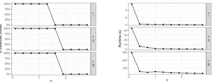
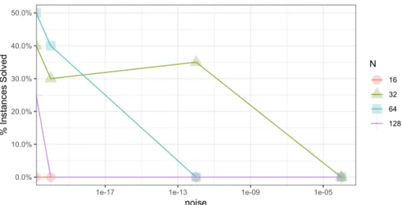
5-1 Average performance and runtime of ELO over 20 instances with 𝑝 = 30 features and 𝑛 = 1, 10, 30 samples. . . 195 5-2 Average performance of LBR algorithm for various noise and truncation levels. . 196

(14)

6-1 The behavior Γ¯_𝑘,𝑘 for 𝑛 = 107 nodes, planted clique of size 𝑘 = 700 ≪ ⌊√𝑛⌋ =

3162 and “high" and “low" values of ¯𝑘. We approximate Γ¯_𝑘,𝑘(𝑧) using the Taylor

ex-pansion ofℎ−1_{by ˜}_Γ_¯ 𝑘,𝑘(𝑧) = 1₂ (︀(︀_𝑘 2 )︀ +(︀𝑧₂)︀)︀+√1 2 √︁(︀(︀_𝑘 2 )︀ −(︀𝑧2 )︀)︀ log[︀(︀𝑘_𝑧)︀(︀𝑛−𝑘¯_𝑘−𝑧 )︀]︀ . To cap-ture the monotonicity behavior, we renormalize and plot (︀¯𝑘)︀−32 (︁_Γ˜

¯

𝑘,𝑘(𝑧)− 12

(︀¯_𝑘 2

)︀)︁ versus the overlap sizes 𝑧 _{∈ [⌊}¯𝑘𝑘_𝑛_{⌋, 𝑘]. . . 231} 6-2 The behavior Γ¯_𝑘,𝑘 for 𝑛 = 107 nodes, planted clique of size 𝑘 = 4000 ≫ ⌊√𝑛⌋ =

3162 and “high" and “low" values of ¯𝑘. The rest of the plotting details are identical with that of Figure 1. . . 233

(15)

List of Tables

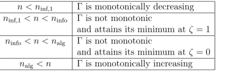
3.1 The phase transition property of the limiting curve Γ (𝜁) . . . 108 6.1 The monotonicity phase transitions of Γ_𝑘,𝑘¯ at 𝑘 =√𝑛 and varying ¯𝑘. . . 222

(16)

(17)

Chapter 1 Introduction

The problem of statistical inference is one of the most fundamental tasks in the field of statistics. The question it studies is the following: assuming one has access to a dataset consisting of samples drawn from an unknown data distribution, can they infer structural properties of the underlying distribution? One of the earliest recorded examples of statistical inference methods can be traced back at least to the early 1800’s. In 1801, Gauss introduced and used the least squares method, a now popular statistical method, to infer the orbits of celestial bodies [Mar77] (as a remark, the least squares method was introduced independently by Legendre in 1805 [Sti81]). In that way, Gauss had major impact in astronomy, as he guided the astronomers of the time to successfully infer the orbit of the newly-then discovered asteroid Ceres [Mar77].

During the 19th and 20th century, statistical inference established its existence as a mathe-matical field of study with the fundamental work of the statisticians Galton, Neyman, Pearson, Fisher and Yule among others (see e.g. some of their fundamental works [Gal85], [Yul97], [Fis22], [NP33]). Furthermore, the field shows an extensive study of classical statistical inference models such as regression, classification and (more recently) network models (see the associated chapters in the book [HTF09] and references therein). One common characteristic in most of this classic work, is that the statistical models considered are assumed to have a relatively small number of features and the focus is on creating statistical estimators which achieve asymptotically opti-mal performance as the sample size becomes arbitrarily large ("grows to infinity"). A common example of such an asymptotic property is statistical consistency, where an estimator is named consistent if it converges to some "fixed" true value, as the sample size grows [HTF09].

(18)

However, in recent years, mostly due to the emergence of the Big Data paradigm, there has been an explosion on the available data which are actively used for various statistical infer-ence tasks across disciplines of sciinfer-ence [BBHL09], [CCL+08], [LDSP08], [QMP+12], [PZHS16], [CWD16]. For example, this has proven a revolutionary fact for many scientific fields from biology [BBHL09], [CCL+08] to electrical engineering [QMP+12], [PZHS16] to social sciences [CWD16]. Naturally, though, the "explosion" of the available data leads to the "explosion" of the feature size which should be taken into account in the "high-dimensional" statistical inference models. This implies that the feature size should grow together with the sample size to infinity. On top of this, in many high dimensional statistical application, such as genomics [BBHL09], [CCL+08] and radar imaging [LDSP08], the feature size is not only comparable with the number of sam-ples, but significantly larger than it. This is exactly the opposite regime to the one which is classically analyzed in statistical inference. These reasons lead to the recent research field of high dimensional statistical inference.

The study of high-dimensional inference is inherently connected with computational ques-tions. The computational challenge is rather evident; the statistical algorithms are now defined on input domains of a very large size and therefore, to produce meaningful outputs in reason-able time, their termination time guarantees should be scalreason-able with respect to the (potentially massive) input’s size. Note that, with high dimensional input, this is a non-trivial consideration as many "textbook" statistically optimal algorithms usually take the form of an, in principle non-convex optimization problem. A standard example is the paradigm of maximum likelihood estimation.

High-dimensionality also leads to multiple statistical and modeling challenges. An important challenge is with respect to the techniques that can be used in that setting: both the classical version of the Central Limit Theorem [Nag76] and the Student-t test [FHY07] have been proven to fail in high dimensional cases. A case in point, which is highly relevant to the results in this thesis, is a modeling challenge in high dimensional linear regression. Specifically, consider the linear regression setting where the statistician observes 𝑛 noisy linear samples of a hidden vector 𝛽* ∈ R𝑝 _{of the form} _{𝑌 = 𝑋𝛽}* _{+ 𝑊 for 𝑋} _{∈ R}𝑛×𝑝 _and _𝑊 _{∈ R}𝑛_{. Note that here}

𝑝 corresponds to the number of features. The goal is to infer the hidden vector 𝛽* _{from the}

(19)

moment high-dimensionality is imposed, a non-identifiability issue arises: even in the extremely optimistic case for the statistician where 𝑊 = 0, 𝛽* _{is simply one out of the infinitely many}

solutions of the underdetermined linear system 𝑌 = 𝑋𝛽*_{. This, in principle, makes inference in}

high dimensional linear regression impossible. In particular, additional assumptions need to be added to the regression model. For example, one of the standard assumptions in the literature of high dimensional linear regression is that the vector 𝛽* _{is sparse, that is most of its entries are}

equal to zero. Under the sparsity assumption, accurate inference indeed becomes possible for 𝑛 much smaller than 𝑝 (see [HTW15] and references therein).

It becomes rather clear from the above discussion that the study of high dimensional statis-tical models require a novel study with respect to both its computational and statisstatis-tical limits. Towards this goal a large body of recent research has been devoted to identifying those limits for various high dimensional statistical models. For example, the following high dimensional mod-els have been analyzed in the literature: the sparse PCA problem, submatrix localization, RIP certification, rank-1 submatrix detection, biclustering, high dimensional linear regression, the tensor PCA problem, Gaussian mixture clustering and the stochastic block model (see [WX18], [BPW18] for two recent surveys and references therein for each model). We start by explicitly stating how the statistical and computational limits are defined for a high dimensional statistical inference problem.

For the statistical limit, the focus is on understanding the sampling complexity (or minimax rates) of the high dimensional statistical models. That is the focus is on the following question, The statistical question: What is the minimum necessary "signal strength" to perform an

accurate statistical inference?

We call the answer to the question above, the statistical limit of the model. Notice that to define statistical limit we assume unbounded computational power for the statistical estimators. For the computational limits, the focus is on computationally efficient estimators. For the results in this thesis we interpet computationally-efficient algorithms as algorithms with termination time being polynomial in the input dimensions. We focus on:

The computational question: What is the minimum necessary "signal strength" to perform an accurate and computationally efficient statistical inference?

(20)

We call the answer to the question above, the computational limit of the model. For many of the mentioned models, the accurate identification of the statistical and computational limits are far from being well-understood.

Despite being far from a complete theory, an interesting phenomenon has been repeatedly observed in the study of high-dimensional statistical models; the statistical limit of the problem appears usually significantly below the smallest known computational limit that is,

statistical limit≪ computational limit.

This phenomenon is called a computational-statistical gap [WX18], [BPW18]. Examples of models where computational-statistical gaps appears include, but are not limited to: the high-dimensional linear regression problem, the planted independent set problem and the planted dense subgraphs problems in sparse Erdős-Rényi graphs, the planted clique problem in dense Erdős-Rényi graphs, the Gaussian bi-clustering problem, the sparse rank-1 submatrix problem, the tensor decomposition problem, the sparse PCA problem, the tensor PCA problem and the stochastic block model (see [BBH18] and references therein).

Computational-statistical gaps provide a decomposition of the parameters space into three (possibly empty) regimes;

∙ (the information-theoretic impossible regime) The regime where the "signal strength" is less than the statistical limit, making inference impossible.

∙ (the algorithmically easy regime) The regime where the "signal strength" is larger than the computational limit so that the inference task is possible and is achieved by computationally efficient methods.

∙ (the apparent algorithmically hard regime) The regime where the "signal strength" is in between the statistical limit and the computational limit, and therefore the inference task is statistically possible but no computationally efficient method is known to succeed. Note that the existence (or non-triviality) of the hard regime is equivalent with the presence of a computational-statistical gap for the model.

(21)

Towards understanding computational-statistical gaps, and specifically identifying the funda-mentally hard region for various inference problems, a couple of approaches have been considered. One of the approaches seeks to identify the algorithmic limit "from above", in the sense of iden-tifying the fundamental limits in the statistical performance of various families of known com-putationally efficient algorithms. Some of the families that have been analyzed are (1) the Sum of Squares (SOS) hierarchy, which is a family of convex relaxation methods [Par00], [Las01] (2) the family of local algorithms inspired by the Belief Propagation with the celebrated example of Approximate Message Passing [DMM09], [DJM13]), (3) the family of statistical query algorithms [Kea98] and (4) several Markov Chain Monte Carlo algorithms such as Metropolis Hasting and Glauber Dynamics [LPW06]. Another approach offers an average-case complexity-theory point of view [BR13], [CLR17], [WBP16], [BBH18]. In this line of work, the hard regimes of the var-ious inference problems are linked by showing that solving certain high dimensional statistical problems in their hard regime reduces in a polynomial time to solving other high dimensional statistical problems in their own hard regime.

In this thesis, we build on a third approach to understand computational-statistical gaps. We study the geometry of the parameter space (we also call it solution space geometry for reasons that are to become apparent) and investigate whether a geometrical phase transition occurs between the easy and the hard regime.

The geometric point of view we follow is motivated from the study of average-case optimiza-tion problems, that is combinatorial optimizaoptimiza-tion problems under random input. These problems are known to exhibit computational-existential gaps; that is there exists a range of values of the objective function which on the one hand are achievable by some feasible solution but on the other hand no computationally efficient method is proven to succeed. The link with the geometry comes out of the observation that for several average-case optimization problems (and their close relatives, random constraint satisfaction problems) an inspiring connection have been drawn be-tween the geometry of the space of feasible solutions and their algorithmic difficulty in the regime where the computational-existential gap appears (the conjectured hard regime). Specifically it has been repeatedly observed that the conjectured algorithmically hard regime for the problem coincides with the appearance of a certain disconnectivity property in the solution space called the Overlap Gap Property (OGP), originated in spin glass theory. Furthermore, it has also been

(22)

seen that at the absence of this property very simple algorithms, such as greedy algorithms can exploit the smooth geometry and succeed. The definition of OGP is motivated by the concen-tration of the associated Gibbs measures [Tal10] for low enough temperature to the optimization problem, and concerns the geometry of the near (optimal) feasible solutions. We postpone the exact definition of OGP to later chapters of this thesis. The connection between the hard regime for the optimization problem and the presence of OGP in the feasible space was initially made in the study of the celebrated example of random𝑘-SAT (independently by [MMZ05], [ACORT11]) but then has been established for other models such as maximum independent set in random graphs [GSa], [RV14].

Note that contrary to statistical inference models, in average-case optimization problems there is no "planted" structured to be inferred and the goal is solely to maximize an objective value among a set of feasible solutions. For this reason, one cannot immediately transfer the literature on the Overlap Gap Property from computational-existential gaps to computational-statistical gaps. Nevertheless, one goal of this thesis is to make this possible by appropriately defining and using the Overlap Gap Property notion to study the computational-statistical gaps. In particular we are interested in the following question,

Can the Overlap Gap Property phase transition explain the appearance of computational-statistical gaps in statistical inference?

The goal of this thesis is to present results for the computational-statistical gaps of two well-studied and fundamental statistical inference problems: the high dimensional linear regression model and the planted clique model.

1.1 The Models: Definitions and Inference Tasks

In this subsection we describe the two high-dimensional statistical models this thesis is focusing on. Our goal to study their computational-statistical gaps.

1.1.1 The High Dimensional Linear Regression Model

As explained in the introduction, fitting linear regression models to perform statistical inference has been the focus of a lot of research work over the last two centuries. Recently the study

(23)

of linear regression has seen a revival of interest from scientists, because of the new challenge of high dimensionality, with applications ranging from compressed sensing [CT05], [Don06] to biomedical imaging [BLH+14], [LDSP08] to sensor networks [QMP+12], [PZHS16] (see also three recent books on the topic [Wai19], [HTW15], [FR13]).

Our first model of study is the high dimensional linear regression model which is a simpli-fied and long-studied mathematical version of high dimensional linear regression. Despite its simplicity, the analysis of the model has prompted various important algorithmic and statistical developments in the recent years, for example the development of the LASSO algorithm [HTW15] and multiple compressed sensing methods [FR13].

We study the high dimensional linear regression model in Chapters 2, 3, 4 and 5. Setting Let𝑛, 𝑝 _{∈ N. Let}

𝑌 = 𝑋𝛽*+ 𝑊 (1.1)

where 𝑋 is a data 𝑛× 𝑝 matrix, 𝑊 is a 𝑛 × 1 noise vector, and 𝛽* _{is the (unknown)} _𝑝_{× 1 vector}

of regression coefficients. We refer to 𝑛 as the number of samples of the model and 𝑝 as the number of features for the model.

Inference Task The inference task is to recover 𝛽* _{from having access only to the data matrix}

𝑋 and the noisy linear observations 𝑌 . The goal is to identify the following two fundamental limits of this problem

∙ the minimum 𝑛 so that statistically accurate inference of 𝛽* _{is possible by using any}

esti-mator (statistical limit) and

∙ the minimum 𝑛 so that statistically accurate inference of 𝛽* _{is possible by using a}

compu-tationally efficient estimator, that is an estimator with worst case termination time being polynomial in 𝑛, 𝑝 (computational limit).

Gaussian Assumptions on 𝑋, 𝑊 Unless otherwise mentioned, we study the problem in the average case where (𝑋, 𝑊 ) are generated randomly where 𝑋 has iid 𝒩 (0, 1) entries and 𝑊 has iid _{𝒩 (0, 𝜎}2). Here and everywhere below by _{𝒩 (𝜇, 𝜎}2_{) we denote the normal distribution on}

(24)

assumptions in the literature, see for example [EACP11], [JBC17], [Wai09b], [Wai09a], [WWR10] and the references in [HTW15, Chapter 11].

Parameters Assumptions The focus is on the high dimensional setting where 𝑛 < 𝑝 and both 𝑝_{→ +∞. The recovery should occur with probability tending to one, with respect to the} randomness of 𝑋, 𝑊 , as 𝑝 → +∞ (w.h.p.). For the whole thesis, we assume that 𝑝 → +∞ and the parameters 𝑛, 𝑘, 𝜎2 _{are sequences indexed by} _{𝑝, 𝑛}

𝑝, 𝑘𝑝, 𝜎2𝑝. The parameters 𝑛, 𝑘, 𝜎2 are

assumed to grow or not to infinity, depending on the specific context.

Structural Assumptions on 𝛽* _{As mentioned in the Introduction, the high-dimensional}

regime is an, in principle, impossible regime for (exact) inference of𝛽* _from_{(𝑌, 𝑋) ; the}

underly-ing linear system, even at the extreme case𝜎 = 0, is underdetermined. For this reason, following a large line of research, we study the model under the additional structural assumptions on the vector 𝛽*_.

Depending on the chapter we make different structural assumption on the vector of coefficients 𝛽*. We mention here the two most common assumptions throughout the different Chapters of this thesis. Unless otherwise specified, we study the high dimensional linear regression model under these assumptions.

First, we assume that the vector of coefficients 𝛽* is 𝑘-sparse, that is the support size of 𝛽* (i.e. the number of regression coefficients with non-zero value) equals to some positive integer parameter𝑘 which is usually taken much smaller than 𝑝. Sparsity is a well-established assumption in the statistics and compressed sensing literature (see for exaple, the books [HTW15, FR13]), with various applications for example in biomedical imaging [BLH+14], [LDSP08] and sensor networks [QMP+12], [PZHS16].

Second, we assume that the non-zero regression coefficients 𝛽_𝑖* are all equal with each other and (after rescaling) equal to one; that is we assume we assume a binary 𝛽* _{∈ {0, 1}}𝑝_{. From a}

theoretical point of view, we consider this more restrictive case to make possible a wider technical development and a more precise mathematical theory. From an applied point of view, the case of binary and more generally discrete-valued𝛽* has received a large interest in the study of wireless communications and information-theory literature [HB98], [HV02], [BB99], [GZ18], [TZP19], [ZTP19]. Finally, recovering a binary vector is equivalent with recovering the support of the

(25)

vector (indices of non-zero coordinates), which is a fundamental question in the literature of the model [TWY12], [OWJ11],[RG13],[Geo12], [Zha93], [MB06a] with various applications such as in gene selection in genomics [HC08], [HG10], [HY09] and radar signal processing [Dud17], [XZB01], [CL99].

Now, we would like to emphasize that in most cases we do not assume a prior distribution on 𝛽*_{; we simply assume that} _𝛽* _{is an arbitrary fixed, yet unknown, structured vector (e.g. a}

binary and 𝑘-sparse vector). This is the setting of interest in Chapters 3, 4 and 5 where the exact structural assumptions are explicitly described. The only time we assume a prior distribution is on Chapter 2 where we assume that 𝛽* _{is chosen according to a uniform prior over the space of}

binary 𝑘-sparse vectors.

1.1.2 The Planted Clique Model

Inferring a hidden community structure in large complex networks has been the focus on multiple recent statistical applications from cognitive science (brain modeling) to web security (worm prop-agation) to biology (protein interactions) and natural language processing [GAM+18, ZCZ+09, PDFV05]

A simplified, yet long-studied, mathematical model for community detection is the planted clique model, first introduced in [Jer92]. Despite its simplicity the model has motivated a large body of algorithmic work and is considered one of the first and most well-studied models for which a computational-statistical gaps appears [WX18, BPW18].

The planted clique model is studied in Chapter 6.

Setting Let 𝑛, 𝑘 ∈ N with 𝑘 ≤ 𝑛. The statistician observes an 𝑛-vertex undirected graph 𝐺 sampled in two stages. In the first stage, the graph is sampled according to an Erdős-Rényi graph 𝐺(︀𝑛,1₂)︀, that is there are 𝑛 vertices and each undirected edges is placed independently with probability 1₂. In the second stage, 𝑘 out of the 𝑛 vertices are chosen uniformly at random and all the edges between these 𝑘 vertices are deterministically added (if they did not already exist due to the first stage sampling). We call the second stage chosen 𝑘-vertex subgraph the planted clique _𝒫𝒞.

(26)

Inference Task The inference task of interest is to recover _{𝒫𝒞 from observing 𝐺. The} computational-statistical gap relies upon identifying the minimum 𝑘 = 𝑘𝑛 so that inference of

𝒫𝒞 is possible by using an arbitrary estimator (statistical limit) and the minimum 𝑘 = 𝑘𝑛so that

inference of _{𝒫𝒞 is possible by a computationally efficient estimator (computational limit). The} statistical limit of the inference task is well-known in the literature to equal 𝑘 = 𝑘𝑛 = 2 log2𝑛.

For this reason, in this thesis we focus on the computational limit of the model.

Parameters Assumptions The focus is on the asymptotic high-dimensional setting where both𝑘 = 𝑘𝑛, 𝑛→ +∞ and the recovery should hold with probability tending to one as 𝑛 → +∞

(w.h.p.).

1.2 Notation

For the rest of the Introduction we require the following mathematical notation. For 𝑝 _{∈ (0, ∞), 𝑑 ∈ N and a vector 𝑥 ∈ R}𝑑 _{we use its} _ℒ

𝑝-norm, ‖𝑥‖𝑝 := (∑︀𝑝_𝑖=1|𝑥𝑖|𝑝)

1 𝑝_{. For}

𝑝 = ∞ we use its infinity norm ‖𝑥‖∞ := max𝑖=1,...,𝑑|𝑥𝑖| and for 𝑝 = 0, its 0-norm ‖𝑥‖0 = |{𝑖 ∈

{1, 2, . . . , 𝑑}|𝑥𝑖 ̸= 0}|. We say that 𝑥 is 𝑘-sparse if ‖𝑥‖0 = 𝑘. We also define the support of 𝑥,

Support (𝑥) :={𝑖 ∈ {1, 2, . . . , 𝑑}|𝑥𝑖 ̸= 0}. For 𝑘 ∈ Z>0 we adopt the notation [𝑘] :={1, 2, . . . , 𝑘}.

Finally with the real function _{log : R}>0 → R we refer everywhere to the natural logarithm. For

𝜇∈ R, 𝜎2 _{> 0 we denote by} _{𝒩 (𝜇, 𝜎}2_{) the normal distribution on the real line with mean 𝜇 and}

variance 𝜎2_{. We use standard asymptotic notation, e.g. for any real-valued sequences} _{𝑎 𝑛}𝑛∈N

and _{𝑏𝑛}𝑛∈N, 𝑎𝑛 = Θ (𝑏𝑛) if there exists an absolute constant 𝑐 > 0 such that 1_𝑐 ≤ |𝑎_𝑏_𝑛𝑛| ≤ 𝑐;

𝑎𝑛 = Ω (𝑏𝑛) or 𝑏𝑛 = 𝑂 (𝑎𝑛) if there exists an absolute constant 𝑐 > 0 such that |𝑎_𝑏𝑛_𝑛| ≥ 𝑐;

𝑎𝑛= 𝜔 (𝑏𝑛) or 𝑏𝑛= 𝑜 (𝑎𝑛) if lim𝑛|𝑎_𝑏_𝑛𝑛| = 0.

1.3 Prior Work and Contribution per Chapter

First, we consider the high dimensional linear regression problem defined in Subsection 1.1.1. As explained in the Introduction, our main goal is to study the existence and properties of the computational-statistical gap of the problem. We study it under the distributional assumptions

(27)

that 𝑋 has iid _{𝒩 (0, 1) entries and 𝑊 has iid 𝒩 (0, 𝜎}2_{) for some parameter 𝜎}2_{. Furthermore we}

assume that 𝛽* _{is a binary}_{𝑘-sparse vector.}

The focus of most of this thesis is on sublinear sparsity levels, that is, using asymptotic notation, 𝑘 = 𝑜 (𝑝). Nevertheless, before diving into specific contributions it is worth pointing out that a great amount of literature has been devoted on the study of the computational-statistical gap in the linear regime where 𝑛, 𝑘, 𝜎 = Θ(𝑝). One line of work has provided upper and lower bounds on the minimum MSE (MMSE) E [‖𝛽*_{− E [𝛽}* _{| 𝑋, 𝑌 ] ‖}2

2] as a function of the

problem parameters, e.g. [ASZ10, RG12, RG13, SC17]. Here and everywhere below for a vector 𝑣 _{∈ R}𝑝 _{we denote by} _‖𝑣‖

2 , √︀∑︀𝑝𝑖=1𝑣𝑖2 it’s ℓ2 norm. Another line of work has derived explicit

formulas for the MMSE. These formulas were first obtained heuristically using the replica method from statistical physics [Tan02, GV05] and later proven rigorously in [RP16, BDMK16]. Finally, another line of work has provided nearly-optimal computationally efficient methods in this setting using Approximate Message Passing [DMM09, DJM13]. However, to our best of knowledge, most of the techniques used in the proportional regime cannot be used to establish similar results when 𝑘 = 𝑜(𝑝) (with notable exceptions such as [RGV17]). Although there has been significant work focusing also on the sublinear sparsity regime, the exact identification of both the computational and the statistical limits in the sublinear regime, remained an outstanding open problem prior to the results of this thesis. We provide below a brief and targeted literature review, postponing a detailed literature review at the beginning of each Chapter, and provide a high-level summary of our contributions.

The statistical limit of High-Dimensional Linear Regression

We start our study with the statistical limit of the problem. To identify the statistical limit we adopt a Bayesian perspective and assume 𝛽* is chosen from the uniform prior over the binary 𝑘-sparse vectors that is uniform on the set _{𝛽* _{∈ {0, 1}}𝑝 _:_‖𝛽*_‖

0 = 𝑘}.

To judge the recovery performance of𝛽* _{from observing}_{(𝑌, 𝑋) we focus on the mean squared}

error (MSE). That is, given an estimator ^𝛽 as a function of (𝑌, 𝑋), define mean squared error as MSE(︁𝛽^)︁, E[︁‖ ^𝛽_{− 𝛽}*_‖2₂]︁,

(28)

where _{‖𝑣‖ denotes the ℓ}2 norm of a vector 𝑣. In our setting, one can simply choose ^𝛽 =

E [𝛽*], which equals 𝑘𝑝(1, 1, . . . , 1)⊤, and obtain a trivial MSE0 = E [‖𝛽*− E [𝛽*]‖ 2

2], which equals

𝑘(︁1₋𝑘_𝑝)︁. We will adopt the following two natural notions of recovery, by comparing the MSE of an estimator ^𝛽 to MSE0.

Definition 1.3.1 (Strong and weak recovery). We say that ^𝛽 = ^𝛽(𝑌, 𝑋)_{∈ R}𝑝 _achieves

∙ strong recovery if lim sup𝑝→∞MSE

(︁ ^

𝛽)︁/MSE0 = 0;

∙ weak recovery if lim sup𝑝→∞MSE

(︁ ^

𝛽)︁/MSE0 < 1.

A series of results studies the statistical, or information-theoretic as it is also called, limit of both the strong and weak recovery problems have appeared in the literature. A crucial value for the sample size appearing in all such results when 𝑘 = 𝑜(𝑝) is

𝑛info =

2𝑘 log𝑝_𝑘 log(︀𝑘

𝜎2 + 1

)︀. (1.2)

For the impossibility direction, previous work [ASZ10, Theorem 5.2], [SC17, Corollary 2] has established that when 𝑛 _{≤ (1 − 𝑜 (1)) 𝑛}info, strong recovery, is information-theoretically

impos-sible and if 𝑛 = 𝑜(𝑛info), weak recovery is impossible. For the achievability direction, Rad in

[Rad11] has proven that for any 𝑘 = 𝑜 (𝑝) and 𝜎2 _{= Θ (1), there exist some large enough}

con-stant 𝐶 > 0 such that if 𝑛 > 𝐶𝑛info then strong recovery is possible with high probability. In a

similar spirit, [AT10, Theorem 1.5] shows that when 𝑘 = 𝑜(𝑝), 𝑘/𝜎2 _{= Θ(1), and 𝑛 > 𝐶}

𝑘/𝜎2𝑛_info

for some large enough 𝐶𝑘/𝜎2 > 0, it is information theoretically possible to weakly recover the

hidden vector.

The literature suggests that the statistical limit is of the order Θ (𝑛info), but (1) it is only

established in very restrictive regimes for the scaling of 𝑘, 𝜎2_{, (2) the distinction between weak}

and strong recovery is rather unclear and finally (3) the identification of the exact constant in front of 𝑛info seems not to be well understood. These considerations raises the main question of

study in Chapter 2;

Question 1: What is the exact statistical limit for strong/weak recovery of 𝛽*_?

(29)

in a very strong sense. We prove that assuming 𝑘 = 𝑜(︀√𝑝)︀, for any positive constant 𝜖 > 0 if the signal-to-noise ratio 𝑘/𝜎2 _{bigger than a sufficiently large constant then,}

∙ when 𝑛 < (1 − 𝜖) 𝑛info weak recovery is impossible, but

∙ when 𝑛 > (1 + 𝜖) 𝑛info strong recovery is possible.

This establishes an "all-or-nothing statistical phase transition". To the best of our knowledge this is the first time such a phase transition is established for a high dimensional inference model.

The computational limit of High-Dimensional Linear Regression

We now turn to the study of the computational-limit for the high-dimensional linear regression model. For these results no prior distribution is assumed on 𝛽* _and _𝛽* _{is assumed to be an}

arbitrary but fixed binary 𝑘-sparse vector. Note that this is a weaker assumption, in the sense that any with high probability property established under such an assumption, immediately transfers to any prior distribution for 𝛽*.

The optimal sample size appearing in the best known computationally efficient results is 𝑛alg =

(︀

2𝑘 + 𝜎2)︀log 𝑝. (1.3)

More specifically, a lot of the literature has analyzed the performance of LASSO, the ℓ1-

con-strained quadratic program:

min

𝛽∈R𝑝{‖𝑌 − 𝑋𝛽‖

2

2+ 𝜆𝑝‖𝛽‖1}, (1.4)

for a tuning parameter 𝜆𝑝 > 0 [Wai09b], [MB06b], [ZY06], [BRT09a]. It is established that

as long as 𝜎 = Θ (1) and 𝑘 grows with 𝑝, if 𝑛 > (1 + 𝜖) 𝑛alg for some fixed 𝜖 > 0, then for

appropriately tuned 𝜆𝑝 the optimal solution of LASSO strongly recovers 𝛽* [Wai09b].

Further-more, a greedy algorithm called Orthogonal Matching Pursuit has also proven to succeed with (1 + 𝜖) 𝑛alg samples [CW11]. To the best of our knowledge, besides decades of research efforts, no

tractable (polynomial-in-𝑛, 𝑝, 𝑘 termination time) algorithms is known outperform LASSO when 𝑘 = 𝑜 (𝑝), in the sense of achieving strong recovery of 𝛽* _with _𝑛 _{≤ 𝑛}

alg samples. This suggest

(30)

At this point, we would like to compare the thresholds 𝑛alg and the information-theoretic

limit 𝑛info given in (1.2). Assuming the signal to noise ratio 𝑘/𝜎2 is sufficiently large, which is

considered in almost all the above results, 𝑛info is significantly smaller than 𝑛alg. This reason

gives rise to the computational-statistical gap which motivates studying the following question in Chapters 3, 4:

Question 2: Is there a fundamental reason for the failure of computationally efficient methods when 𝑛 ∈ [𝑛info, 𝑛alg]?

We offer a geometrical explanation for the gap by identifying 𝑛alg as the, up-to-constants,

Overlap Gap Property phase transition point of the model. Specifically, we consider the least squares optimization problem defined by the Maximum Likelihood Estimation (MLE) problem;

(MLE) min 𝑛−1

2‖𝑌 − 𝑋𝛽‖₂

s.t. 𝛽 ∈ {0, 1}𝑝

‖𝛽‖0 = 𝑘.

As explained in the Introduction, geometry and the Overlap Gap Property has played crucial role towards understanding several computational-existential gaps for average-case optimization problems. Note that (MLE) is an average-case optimization problem with random input (𝑌, 𝑋). We study it first with respect to optimality; we prove that as long as 𝑛 _{≥ (1 + 𝜖) 𝑛}info, under

certain assumption on the parameters, the optimal solution of (MLE) equals 𝛽*_{, up to negligible}

Hamming distance error. Hence (MLE) is an average-case optimization problem with optimal solution almost equal to 𝛽*_{. Thus, in light of the discussion above, it is expected to be}

algorith-mically hard to solve to optimality when 𝑛 < 𝑛alg. For this reason we appropriately define and

study the presence of the Overlap Gap Property (OGP) in the solution space of (MLE) in the regime 𝑛 _{∈ [𝑛}info, 𝑛alg] and 𝑛 > 𝑛alg. We say that OGP holds in the solution space of (MLE)

if the nearly optimal solutions of (MLE) have only either high or low Hamming distance to 𝛽*_,

and therefore the possible Hamming distances ( "overlaps" ) to 𝛽* _{exhibit gaps. We direct the}

reader to Chapter 3 for the the exact definition of OGP and more references. We show that for some constants 𝑐, 𝐶 > 0,

(31)

∙ when 𝑛 > 𝐶𝑛alg OGP does not hold in the solution space of(MLE) (Chapter 4).

This provides evidence that the high dimensional linear regression recovery problem corresponds to an algorithmically hard problem in the regime 𝑛 < 𝑐𝑛alg. In Chapter 3 we support the

hardness conjecture by establishing that the LASSO not only provably fails to recover exactly the support in the regime 𝑛 < 𝑐𝑛alg, but in the same regime it fails to achieve a different notion

of recovery called ℓ2-stable recovery. In Chapter 4 besides establishing that OGP does not hold,

we also perform a direct local analysis of the optimization problem (MLE) proving that (1) when 𝑛 > 𝐶𝑛alg the optimization landscape is extremely "smooth" to the extent that the only local

minimum (under the Hamming distance metric between the binary𝛽’s) is the global minimum 𝛽*

and (2) the success of a greedy local search algorithm with arbitrary initialization for recovering 𝛽* _when _{𝑛 > 𝐶𝑛}

alg.

The Noiseless High-Dimensional Linear Regression

An admittedly extreme, yet broadly studied, case in the literature of high dimensional linear regression is when the noise level 𝜎 is extremely small, or even zero (also known as the noiseless regime). In this case, the statistical limit of the problem 𝑛info, defined in (1.2), trivializes to

zero. In particular, our results in Chapter 2 imply that one can strongly recover information-theoretically a sparse binary 𝑝-dimensional 𝛽* with 𝑛 = 1 sample, as 𝑝 → +∞. Notice that in this regime the statistical-computational gap becomes even more profound: 𝑛info = 1 and

when 𝜎 = 0 according to (1.3) 𝑛alg = 2𝑘 log 𝑝 remains of the order of 𝑘 log 𝑝. Moreover Donoho

in [Don06] establishes that Basis Pursuit, a well-studied Linear Program recovery mechanism, fails in the noiseless regime 𝜎 = 0 with 𝑛 ≤ (1 − 𝜖)𝑛alg samples for any fixed 𝜖 > 0. On

top of this, our Overlap Gap Property phase transition result described below in Question 2, suggests that the geometry of the sparse binary vectors is rather complex at 𝜎 = 0 for any 𝑛 with 𝑛info= 1 ≤ 𝑛 < 𝑛alg.

On the other hand, the absence of noise makes the model significantly simpler ; it simply is an underdetermined linear system. The linear structure allows the suggestion and rigorous analysis of various computationally efficient mechanisms, moving potentially beyond the standard algorithmic literature of the linear regression model which, as explained in the Introduction, usually is based on either local or convex relaxation methods. These considerations lead to the

(32)

following question which is investigated in Chapter 5:

Question 3: Is there a way to achieve computationally-efficient recovery with 𝑛 < 𝑛alg = 2𝑘 log 𝑝 samples, in the "extreme" noiseless regime 𝜎 = 0?

We answer this question affirmatively by showing that computational efficient estimation is possible even when 𝑛 = 1. We do this by proposing a novel computationally efficient method using the celebrated Lenstra-Lenstra-Lovasz (LLL) lattice basis reduction algorithm (LLL was introduced in [LLL82] for factoring polynomials with rational coefficients). We establish that our recovery method can provably recover the vector 𝛽* with access only to one sample, 𝑛 = 1, and 𝑝_{→ +∞. This profoundly breaks the algorithmic barrier 𝑛}alg of the local search and convex

relaxation method (e.g. LASSO) in the literature. Our proposed algorithm heavily relies on the integrality assumption on the regression coefficients, which trivially holds since 𝛽* _{is assumed to}

be binary-valued. In particular, as opposed to Chapters 2, 3, 4, we do not expect the results in Chapter 5 to generalize to the real-valued case. Interestingly, though, our algorithm does not depend at all to the sparsity assumption on 𝛽* to be successful; it works for any integer-valued 𝛽*_{. We consider the independence of our proposed algorithm to the sparsity assumption}

a fundamental reason for its success. In that way the algorithm does not need to "navigate" in the complex landscape of the binary sparse vectors where Overlap Gap Property holds, avoiding the conjectured algorithmic barrier in this case.

The computational-statistical gap of the Planted Clique Model

We now proceed with discussing our results for the planted clique problem defined in Subsection 1.1.2. As said in the definition of the model, our goal is to provide an explanation for the computational-statistical gap of this model as well.

The statistical limit of the model is exactly known in the literature to be 𝑘 = 𝑘𝑛 = 2 log2𝑛

(see e.g. [Bol85]): if𝑘 < (2− 𝜖) log2𝑛 then it is impossible to recover𝒫𝒞, but if 𝑘 ≥ (2 + 𝜖) log2𝑛

the recovery of _{𝒫𝒞 is possible by a brute-force algorithm. Here and everywhere below by log}₂ we refer to the logarithm function with base 2. It is further known that if 𝑘 ≥ (2 + 𝜖) log2𝑛,

a relatively simple quasipolynomial-time algorithm, that is an algorithm with termination time 𝑛𝑂(log 𝑛)_{, also recovers} _{𝒫𝒞 correctly (see the discussion in [FGR}+_{17] and references therein). On}

(33)

the other hand, recovering _{𝒫𝒞 with a computationally-efficient (polynomial-in-𝑛 time) method} appears much more challenging. A fundamental work [AKS98] proved that a polynomial-time algorithm based on spectral methods recovers _{𝒫𝒞 when 𝑘 ≥ 𝑐}√𝑛 for any fixed 𝑐 > 0 (see also [FR10], [DM], [DGGP14] and references therein.) Furthermore, in the regime𝑘/√𝑛_{→ 0, various} computational barriers have been established for the success of certain classes of polynomial-time algorithms [BHK+16], [Jer92], [FGR+17]. Nevertheless, no general algorithmic barrier such as worst-case complexity-theoretic barriers has been proven for recovering _{𝒫𝒞 when 𝑘/}√𝑛 _{→ 0.} The absence of polynomial-time algorithms together with the absence of a complexity-theory explanation in the regime where 𝑘 _{≥ (2 + 𝜖) log}₂𝑛 and 𝑘/√𝑛 _{→ 0 gives rise to arguably one of} the most celebrated and well-studied computational-statistical gaps in the literature, known as the planted clique problem.

As described below Question 2, in Chapters 3, 4 we carefully define and establish an Overlap Gap Property phase transition result for the high dimensional linear regression problem. In that way we provide a possible explanation for the conjectured algorithmic hardness. This suggests the following question which we study in Chapter 6.

Question 4: Is there an Overlap Gap Property phase transition explaining the conjectured algorithmic hardness of recovering _{𝒫𝒞 when 𝑘/}√𝑛→ 0?

We provide strong evidence that the answer to the above question is affirmative. We consider the landscape of the dense subgraphs of the observed graph, that is subgraphs with nearly maximal number of edges. We study their possible intersection sizes ( "overlaps" ) with the planted clique. Using the first moment method, as an non-rigorous approximation technique, we provide evidence of a phase transition for the presence of Overlap Gap Property (OGP) exactly at the algorithmic threshold 𝑘 = Θ (√𝑛). More specifically, we say that OGP happens in the landscape of dense subgraphs of the observed graph if any sufficiently dense subgraph has either high or low overlap with the planted clique. We direct the reader to the Introduction of Chapter 6 for the the exact definition of OGP. We provide evidence that

∙ when 𝑘 = 𝑜 (√𝑛) OGP holds in the landscape of dense subgraphs, and ∙ when 𝑘 = 𝜔 (√𝑛) OGP does not hold in the landscape of dense subgraphs.

(34)

We prove parts of the conjecture such as the presence of OGP when 𝑘 is a small positive power of 𝑛 by using a conditional second moment method. We expect the complete proof of the conjectured OGP phase transition to be a challenging but important part towards understanding the algorithmic difficulty of the planted clique problem.

1.4 Technical Contributions

Various technical results are established towards proving the results presented in Section 1.3. In this Section, we describe two of the key technical results obtained towards establishing two of the most important results presented in this thesis: the presence of the Overlap Gap Property for the high dimensional linear regression mode (Chapter 3) and for the planted clique model (Chapter 6). The results are of fundamental nature and can be phrased independently from the Overlap Gap Property or any statistical context, and are of potential independent mathematical interest.

The Gaussian Closest Vector Problem

In Chapter 3 and the study of the Overlap Gap Property for the high dimensional linear regression model the following random geometry question naturally arises.

Let 𝑛, 𝑝_{∈ N and ℬ := {𝛽 ∈ {0, 1}}𝑝 _: _‖𝛽‖

0 = 𝑘} the set of all binary 𝑘-sparse vectors in R𝑝.

Suppose𝑋 ∈ R𝑛×𝑝 _{has i.i.d.} _{𝒩 (0, 1) entries and 𝑌 ∈ R}𝑛×𝑝 _{has i.i.d.} _{𝒩 (0, 𝜎}2_{) entries. We would}

like to understand the asymptotic behavior of the following minimization problem, min

𝛽∈ℬ𝑛

−1/2_{‖𝑌 − 𝑋𝛽‖}

2 (1.5)

subject to specific scaling of𝜎2_{, 𝑘, 𝑛, 𝑝 as they grow together to infinity. In words, (1.5) estimates}

how well some vector of the form 𝑋𝛽, 𝛽 _{∈ ℬ approximate in (rescaled) ℓ}2 error a target vector

𝑌 .

The focus is on 𝜎2 _{= Θ (𝑘), which makes the per-coordinate variance of 𝑌 , which equals to}

𝜎2_{, comparable with the per-coordinate variance of} _{𝑋𝛽, which equals 𝑘. Studying the extrema}

(35)

develop-ment of fundadevelop-mental tools such as Slepian’s, Sudakov-Fernique and Gordon’s inequalities [Ver18, Section 7.2], with multiple applications in spin glass theory [Tal10], compressed sensing [OTH13] and in information theory [ZTP19, TZP19]. The problem can also be motivated in statistics as an "overfitting test"; it corresponds to the fundamental limits of fitting a sparse binary linear model to an independent random vector of observations.

Now if 𝑛 = Ω(︀𝑘 log𝑝_𝑘)︀ then a well-studied random matrix property, called the Restricted Isometry Property (RIP) is known to hold for the random matrix𝑋. The RIP states that for any 𝑘-sparse vector 𝑣, it holds 𝑛−1/2_{‖𝑋𝑣‖}

2 ≈ ‖𝑣‖2 with probability tending to one as 𝑛, 𝑝, 𝑘 → +∞

(see e.g. [FR13, Chapter 6]). Here and everywhere in this Section, the approximation sign should be understood as equality up to a multiplicative constant. Now, if 𝑛 = Ω(︀𝑘 log𝑝_𝑘)︀, using the RIP and 𝜎2 _{= Θ (𝑘) it is a relatively straightforward exercise that}

min 𝛽∈ℬ 𝑛 −1/2_{‖𝑌 − 𝑋𝛽‖} 2 ≈ √ 𝑘 + 𝜎2_, _(1.6)

as 𝑛, 𝑝, 𝑘_{→ +∞. Here}√𝑘 + 𝜎2 _{simply corresponds to the variance per coordinate of any vector}

of the form 𝑌 _{− 𝑋𝛽 for 𝛽 ∈ ℬ.}

On the other hand, when𝑛 = 𝑜(︀𝑘 log𝑝_𝑘)︀𝑋 is known not to satisfy RIP and to the best of our knowledge no other tool provides tight results for the value of the optimization problem (1.5). In Chapter 3 we study the following question:

Question: Which value does (1.5) concentrate on when 𝑛 = 𝑜(︀𝑘 log𝑝_𝑘)︀?

We answer this question under the assumption that 𝑛 satisfies 𝑛 _{≤ 𝑐𝑘 log} 𝑝_𝑘 for some small constant 𝑐 > 0 but also 𝑘 log 𝑘 ≤ 𝑛. Notice that naturally restricts 𝑘 to be at most 𝑝1+𝑐𝑐 _{for the}

small constant 𝑐 > 0. We show under these assumptions that min 𝛽∈ℬ𝑛 −1/2_{‖𝑌 − 𝑋𝛽‖} 2 ≈ √ 𝑘 + 𝜎2_exp (︂ −𝑘 log 𝑝 𝑘 𝑛 )︂ ,

as 𝑛, 𝑝, 𝑘 → +∞. Comparing with (1.6) we see that the behavior of (1.5) in the regime 𝑛 = 𝑜(︀𝑘 log_𝑘𝑝)︀differs from the regime 𝑛 = Ω(︀𝑘 log𝑝_𝑘)︀ by an exponential factor in ₋𝑘 log

𝑝 𝑘

𝑛 . The exact

(36)

The Densest Subgraph Problem in Erdős-Rényi random graphs

In Chapter 6 and the study of the Overlap Gap Property for the planted clique model the following random graph theory question naturally arises. Consider an𝑛-vertex undirected graph 𝐺 sampled from the Erdős-Rényi model 𝐺(︀𝑛,1

2

)︀

, that is each edge appears independently with probability

1

2. We would like to understand the concentration properties of the𝐾-Densest subgraph problem,

𝑑ER,𝐾(𝐺) = max

𝐶⊆𝑉 (𝐺),|𝐶|=𝐾|𝐸[𝐶]|, (1.7)

where 𝑉 (𝐺) denotes the set of vertices of 𝐺 and for any 𝐶 _{⊆ 𝑉 (𝐺), 𝐸[𝐶] denotes the set of} induced edges in 𝐺 between the vertices of 𝐶. In words, (1.7) is the maximum number of edges of a 𝐾-vertex subgraph of 𝐺.

The study of𝑑ER,𝐾(𝐺) is an admittedly natural question in random graph theory which, to the

best of our knowledge, remains not well-understood even for moderately large values of 𝐾 = 𝐾𝑛.

It should be noted that this is in sharp contrast with other combinatorial optimization questions in Erdős-Rényi graphs, such as the size of the maximum clique or the chromatic number, where tight results are known [Bol85, Chapter 11].

We describe briefly the literature of the problem. For small enough values of 𝐾, specifically 𝐾 < 2 log₂𝑛, it is well-known that a clique of size 𝐾 exists and therefore 𝑑ER,𝐾(𝐺) =

(︀_𝐾

2

)︀

w.h.p. as 𝑛→ +∞ [GM75]. On the other hand when 𝐾 = 𝑛, trivially 𝑑ER,𝐾(𝐺) follows Binom

(︀(︀𝐾 2

)︀ ,1₂)︀ and hence for any 𝛼𝐾 → +∞, 𝑑ER,𝐾(𝐺) = 1₂

(︀_𝐾

2

)︀

+ 𝑂 (𝐾𝛼𝐾) w.h.p. as 𝑛 → +∞. In Chapter 6

we study the following question:

Question: How does 𝑑ER,𝐾(𝐺) behave asymptotically when 2 log2𝑛 ≤ 𝐾 = 𝑜 (𝑛)?

A recent result in the literature studies the case 𝐾 = 𝐶 log 𝑛 for 𝐶 > 2 [BBSV18] and establishes (it is an easy corollary of the main result of [BBSV18]),

𝑑ER,𝐾(𝐺) = ℎ−1 (︂ log 2− 2 (1 + 𝑜 (1)) 𝐶 )︂ (︂ 𝑘 2 )︂ , (1.8)

w.h.p. as 𝑛 _{→ +∞. Here log is natural logarithm and ℎ}−1 _{is the inverse of the (rescaled)}

binary entropy ℎ : [1₂, 0] → [0, 1] is defined by ℎ(𝑥) = −𝑥 log 𝑥 − (1 − 𝑥) log 𝑥. Notice that lim𝐶→+∞ℎ−1

(︁

log 2₋ 2(1+𝑜(1))_𝐶 )︁= 1

(37)

first order behavior of 𝑑ER,𝐾(𝐺) at " very large" 𝐾 such as 𝐾 = 𝑛.

In Chapter 6 we obtain results on the behavior of𝑑ER,𝐾(𝐺) for any 𝐾 = 𝑛𝐶, for 𝐶∈ (0, 1/2).

Specifically in Theorem 6.2.10 we show that for any 𝐾 = 𝑛𝐶 _for _𝐶 _{∈ (0, 1/2) there exists some}

positive constant 𝛽 = 𝛽(𝐶)∈ (0,3 2) such that 𝑑ER,𝐾(𝐺) = ℎ−1 (︃ log 2− log (︀𝑛 𝐾 )︀ (︀_𝐾 2 )︀ )︃ (︂ 𝐾 2 )︂ − 𝑂(︁𝐾𝛽√︀log 𝑛)︁ (1.9) w.h.p. as 𝑛_{→ +∞.}

First notice that as our result are established when𝐾 is a power 𝑛 it does not apply in the logarithmic regime. Nevertheless, it is in agreement with the result of of [BBSV18] since for 𝐾 = 𝐶 log 𝑛, log(︀_𝐾𝑛)︀ (︀𝐾 2 )︀ = (1 + 𝑜 (1))𝐾 log (︀_𝑛 𝐾 )︀ 𝐾2 2 = (1 + 𝑜 (1))2 𝐶,

that is the argument in ℎ−1 _{of (1.9) converges to the argument in} _ℎ−1 _{of (1.8) at this scaling.}

Finally, by Taylor expanding ℎ−1 _around _{log 2 and using (1.9) we can identify the second}

order behavior of 𝑑ER,𝐾(𝐺) for 𝐾 = 𝑛𝐶, for 𝐶∈ (0, 1/2) to be,

𝑑ER,𝐾(𝐺) = 1 2 (︂ 𝐾 2 )︂ +𝐾 3 2 √︁ log(︀𝑛 𝐾 )︀ 2 + 𝑜 (︁ 𝐾32 )︁ , w.h.p. as 𝑛_{→ +∞.}

The exact statements and proofs of the above results can be found in Chapter 6.

1.5 Organization and Bibliographic Information

Most results described in this thesis have already appeared in existing publications, which we briefly mention below.

Chapter 2 presents new results on the statistical limit of the high dimensional linear regres-sion model. It presents an exact calculation of the statistical limit of the model, and reveals a strong "all-to-nothing" information-theoretic phase transition of the model. The results of this Chapter are included in the paper with title "The All-or-Nothing Phenomenon in Sparse Linear Regression" which is joint work with Galen Reeves and Jiaming Xu and appeared in the

(38)

Proceedings of the Conference on Learning Theory (COLT) 2019 [RXZ19].

Chapter 3 establishes the presence of the Overlap Gap Property in the conjectured hard regime for high dimensional linear regression. This is based on the paper "High dimensional linear regression with binary coefficients: Mean squared error and a phase transition" which is joint work with David Gamarnik and appeared in the Proceedings of the Conference on Learning Theory (COLT) 2017 [GZ17a].

Chapter 4 proves the absence of the Overlap Gap Property in the algorithmically easy regime for high dimensional linear regression. Moreover, it shows the success of a greedy Local Search method also in the easy regime. This is based on the paper "Sparse High Dimensional Linear Regression: Algorithmic Barrier and a Local Search Algorithm" which is joint work with David Gamarnik and is currently available as a preprint [GZ17b].

Chapter 5 offers a new computationally-efficient recovery method for noiseless high dimen-sional linear regression using lattice basis reduction. The algorithm provably infers the hidden vector even with access to only one sample. This is based on the paper "High dimensional linear regression using Lattice Basis Reduction" which is joint work with David Gamarnik and appeared in the Advances of Neural Information Processing Systems (NeurIPS) 2018 [GZ18].

Chapter 6 presents strong evidence that Overlap Gap Property for the planted clique model appears exactly at the conjectured algorithmic hard regime for the model. It also offers a proof of the presence of the Overlap Gap Property in a part of the hard regime. This is based on the paper "The Landscape of the Planted Clique Problem: Dense Subgraphs and the Overlap Gap Property" which is joint work with David Gamarnik and is currently available as a preprint [GZ19].

Other papers by the author over the course of his PhD that are not included in this thesis are [ZTP19, TZP19, LVZ17, MSZ18, LVZ18, BCSZ18].

(39)

Chapter 2 The Statistical Limit of High Dimensional

Linear Regression. An All-or-Nothing

Phase Transition.

2.1 Introduction

In this Chapter, we study the statistical, or information-theoretic, limits of the high-dimensional linear regression problem (defined in Subsection 1.1.1) under the following assumptions. For 𝑛, 𝑝, 𝑘 _{∈ N with 𝑘 ≤ 𝑝 and 𝜎}2 _{> 0 we consider two independent matrices 𝑋} _{∈ R}𝑛×𝑝 _and

𝑊 ∈ R𝑛×1 _with _𝑋 𝑖𝑗 i.i.d. ∼ 𝒩 (0, 1) and 𝑊𝑖 i.i.d. ∼ 𝒩 (0, 𝜎2_{), and observe} 𝑌 = 𝑋𝛽*+ 𝑊, (2.1)

where 𝛽* _{is assumed to be uniformly chosen at random from the set} _{{𝑣 ∈ {0, 1}}𝑝 _: _‖𝑣‖

0 = 𝑘}

and independent of (𝑋, 𝑊 ). The problem of interest is to recover 𝛽* _{given the knowledge of} _𝑋

and 𝑌 . Our focus will be on identifying the minimal sample size 𝑛 for which the recovery is information-theoretic possible.

The problem of recovering the support of a hidden sparse vector 𝛽* ∈ R𝑝 _{given noisy}

lin-ear observations has been extensively analyzed in the literature, as it naturally arises in many contexts including subset regression, e.g. [CH90], signal denoising, e.g. [CDS01], compressive

Computational and statistical challenges in high dimensional statistical models

Computational and statistical challenges

in high dimensional statistical models

by

Ilias Zadik

B.A., National Kapodistrean University of Athens (2013)

M.A.St., University of Cambridge (2014)

Submitted to the Sloan School of Management

in partial fulfillment of the requirements for the degree of

Doctor of Philosophy in Operations Research

at the

MASSACHUSETTS INSTITUTE OF TECHNOLOGY

September 2019

c

○ Massachusetts Institute of Technology 2019. All rights reserved.

Author . . . .

Sloan School of Management

July 6, 2019

Certified by . . . .

David Gamarnik

Professor of Operations Research

Thesis Supervisor

Accepted by . . . .

Patrick Jaillet

Dugald C. Jackson Professor

Co-Director, Operations Research Center

Computational and statistical challenges

in high dimensional statistical models

by

Ilias Zadik

Abstract

Acknowledgments

Contents

List of Figures

List of Tables

Chapter 1

Introduction

1.1

The Models: Definitions and Inference Tasks

1.1.1

The High Dimensional Linear Regression Model

1.1.2

The Planted Clique Model

1.2

Notation

1.3

Prior Work and Contribution per Chapter

The statistical limit of High-Dimensional Linear Regression

The computational limit of High-Dimensional Linear Regression

The Noiseless High-Dimensional Linear Regression

The computational-statistical gap of the Planted Clique Model

1.4

Technical Contributions

The Gaussian Closest Vector Problem

The Densest Subgraph Problem in Erdős-Rényi random graphs

1.5

Organization and Bibliographic Information

Chapter 2

The Statistical Limit of High Dimensional

Linear Regression. An All-or-Nothing

Phase Transition.

2.1

Introduction