HAL Id: hal-00881773
https://hal.archives-ouvertes.fr/hal-00881773
Submitted on 8 Nov 2013
HAL is a multi-disciplinary open access
archive for the deposit and dissemination of
sci-entific research documents, whether they are
pub-lished or not. The documents may come from
teaching and research institutions in France or
abroad, or from public or private research centers.
L’archive ouverte pluridisciplinaire HAL, est
destinée au dépôt et à la diffusion de documents
scientifiques de niveau recherche, publiés ou non,
émanant des établissements d’enseignement et de
recherche français ou étrangers, des laboratoires
publics ou privés.
New Iterative Ray-Traced Collision Detection Algorithm
for GPU Architectures
François Lehericey, Valérie Gouranton, Bruno Arnaldi
To cite this version:
François Lehericey, Valérie Gouranton, Bruno Arnaldi. New Iterative Ray-Traced Collision Detection
Algorithm for GPU Architectures. VRST, 2013, Singapore. pp.215-218. �hal-00881773�
New Iterative Ray-Traced Collision Detection Algorithm for GPU Architectures
Franc¸ois Lehericey∗ Val´erie Gouranton† Bruno Arnaldi‡INSA de Rennes, IRISA, Inria
Campus de Beaulieu, 35042 Rennes cedex, France
Abstract
We present IRTCD, a novel Iterative Ray-Traced Collision Detec-tion algorithm that exploits spatial and temporal coherency. Our approach uses any existing standard ray-tracing algorithm and we propose an iterative algorithm that updates the previous time step results at a lower cost with some approximations. Applied for rigid bodies, our iterative algorithm accelerate the collision detection by a speedup up to 33 times compared to non-iterative algorithms on GPU.
CR Categories: I.3.1 [Computer Graphics]: Hardware Architecture—Parallel processing I.3.5 [Computer Graphics]: Computational Geometry and Object Modeling—Physically based modeling
Keywords: Real-Time Physics-based Modeling, Collision Detec-tion, Narrow Phase, Ray-tracing
1
Introduction
In Virtual Reality and others applications of 3D environments, col-lision detection is an essential task and is often considered as a bot-tleneck. Given a set of objects, those which might collide have to be known. This task is complex because of the real-time constraint imposed by the direct interaction of the user and the natural com-plexity (O(n2)) of the naive algorithms. In the recent years, new
approaches using GPGPU (General-Purpose computing on Graphic Processing Unit) have emerged taking advantage of the GPU com-putational performances [Avril et al. 2011]. Our contribution is IRTCD, a new Iterative Ray-Traced Collision Detection algorithm that exploits spatial and temporal coherency.
The paper is organized as follows: Section 2 presents related work. Section 3 details our iterative ray-tracing algorithm. Section 4 describes performance improvements in our experimental scenes. Section 5 concludes this paper and gives future work.
2
Related Work
In this section we present the most relevant literature to our work. For a deeper introduction we suggest the reader to refer to surveys on the topic [Teschner et al. 2005; Kockara et al. 2007]. In 1993, Hubbard [Hubbard 1993] proposed to decompose collision detec-tion in two phases, the broad-phase and the narrow-phase.
∗[email protected] †[email protected] ‡[email protected]
The broad phase takes a set of objects as inputs and outputs a set of potentially colliding pairs. Nowadays this phase is less critical than the narrow phase for performance. Aside brute force, broad phase algorithms can be classified in three categories: spatial partitioning, kinematic and topology.
The narrow phase takes the pairs produced by the broad phase and performs an accurate collision test. It outputs a set of colliding objects and information about the contacts between objects for the physical response. Narrow phase algorithms can be classified in four categories: feature-based, simplex-based, bounding volume hi-erarchy and image based.
This paper focuses on image-based collision detection in the narrow phase, in particular ray-tracing techniques.
Hermann et al. [Hermann et al. 2008] proposed to detect collision by casting rays from the vertices of the objects. Rays are cast from each vertex of each object in the opposite direction of their normal. If a ray hits the inside of the other object before leaving the source object then a collision is detected (see Figure 1).
Figure 1: Hermann et al. algorithm in 2D
The advantage of this algorithm is the information given for phys-ical response. Hermann et al. algorithm gives for each penetrating vertex a direction and a distance to separate the two objects (as can be seen in Figure 1). These distances can be use to compute the physical response without the need of post-processing.
3
Iterative Ray-Traced Collision Detection
Collision detection has to be performed at each simulation step. With ray-traced techniques, rays are cast from scratch at each simulation step for each pair of objects. Instead we propose to use an iterative ray-tracing technique that takes advantage of the temporal coherency between the objects in each pair. Based on Hermann et al. algorithm, our algorithm is used when the relative displacement between objects is under a threshold, the displacementT hreshold (cf. Section 3.3).
In this section we present our iterative ray-traced technique. This technique can be used to speed up collision detection that is valid for both convex and concave objects. Section 3.1 presents the over-all principle of the technique for triangle meshes. Section 3.2 fo-cuses on the ray/triangle intersection. Section 3.3 explains the cri-terion to jump between iterative to non-iterative technique. Section 3.4 justifies why our iterative ray-tracing technique can be used with concave objects and why we can tolerate missed rays. Section 3.5 explains how we use GPU to increase performance.
3.1 Iterative Ray/Triangle-Mesh Intersection
The main idea of iterative ray/triangle-mesh intersection is to use the standard algorithm to get the first intersection and to use an iterative algorithm on the next steps to update the previous result. The standard algorithm can be any algorithm, the only important modification is to record for each ray the reference of the impacted triangle.
Our algorithm relies on an adjacency list between each triangle through the edges. For each ray, the iterative algorithm starts from the previous impacted triangle and tries to follow the path of the ray on the triangle mesh (cf Algorithm 1). We cast the ray into the previously impacted triangle, we then have two cases:
• The ray hits the triangle. The algorithm stops and the inter-section is found.
• The ray misses the triangle. We select the edge that is the clos-est to the ray (explained in section 3.2), get the corresponding triangle through the adjacency list and reiterate the algorithm.
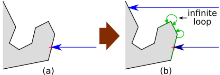
When the ray does not hit the previous triangle, the algorithm iter-ates through the neighboring triangle to locate the intersecting one. Figure 2 shows an example, in (a) the intersection between the ray and the mesh is found with a standard algorithm, in (b) we start from the previous intersection and follow the green path to locate the new intersection. The algorithm may enter in an endless loop if the ray does not hit the mesh anymore or if the path of the ray goes through a concave zone . A case of a trapped ray is exposed in Figure 3. In (a), the intersection is found with a standard algorithm. In (b), we start from the previous intersection but due to a cavity in the geometry the algorithm falls in an infinite loop.
Algorithm 1 Iterative ray/triangle-mesh intersection
functionITRAYTRIINTERSECTION(Ray ray, Triangle tri) for i= 1 → maxIt do ⊲ limit the number of indirection
intersection← cast ray on tri if ray hits tri then
return intersection else
edge← closestEdge(tri, ray) tri← adjacentT riangle(tri, edge) end if
end for
return intertsectionN otF ound end function
(a) (b)
Figure 2: Iterative ray-tracing on a mesh.
The solution to avoid an endless loop is to check if the current tri-angle has already been visited. This solution detects as quickly as possible a loop but is very expensive. A lighter solution is to set a maximum number of iterations with a constant maxIt. Equation 1 gives the value of maxIt that depends on the average size of the triangles in the scene, the displacement threshold that bounds the
(a) (b)
infinite loop
Figure 3: Iterative ray trapped in a concave area.
usage of our iterative algorithm and a confidence level of at least 1.
maxIt= conf idence ×displacementT hreshold averageT rianglesSize (1)
3.2 Ray/Triangle Intersection
We want to compute the intersection point between a ray and a tri-angle. When the ray misses the triangle we want to know which edge is the closest. This problem can be simplified by projecting the ray on the plane that holds the triangle, we then have two cases: • The ray is parallel to the plane, this is a degenerate case and
the ray is discarded.
• The ray is not parallel to the plane, the projection of the ray on the plane gives one intersection point.
Then we check if the intersection point is inside the triangle and otherwise which edge of the triangle is the closest. The distance between a point and an edge is considered as the distance between the point and the closest point of the edge.
Figure 4a shows the different regions on the triangle plane. In the A-region the point is inside the triangle, collision is detected. In the B-regions, the point is outside the triangle and the intersection point is closer to one edge than others (for instance all the points in the B3-region are closer to the edge 3 than to the edge 1 and 2). In the C-regions the point is outside the triangle and the intersection point is equally distant from two edges, in this case we can select any of the two edges (for instance in the C2-region all the points are at the same distance from the edge 1 and 2).
1 2 3 1 2 3
(a)
(b)
B1
B2
B3
C1
A
C2
C3
A
Figure 4: Triangle plane with numerated edges.
Moller et al. [M¨oller and Trumbore 1997] proposed to compute the intersection point of a ray and a triangle in the object space. The result is a vector(t, u, v)⊤
where t is the length of the ray and (u, v)⊤
is the coordinate of the intersection point on the triangle. This vector must satisfy four conditions: u >= 0, v >= 0, u + v <= 1 and t >= 0.
We propose to generalize this algorithm to get the closest edge by following the Algorithm 2. This algorithm leads to the region
sented in Figure 4b. These regions are compatible with those pre-sented in Figure 4a, with an arbitrary choice taken in the C regions.
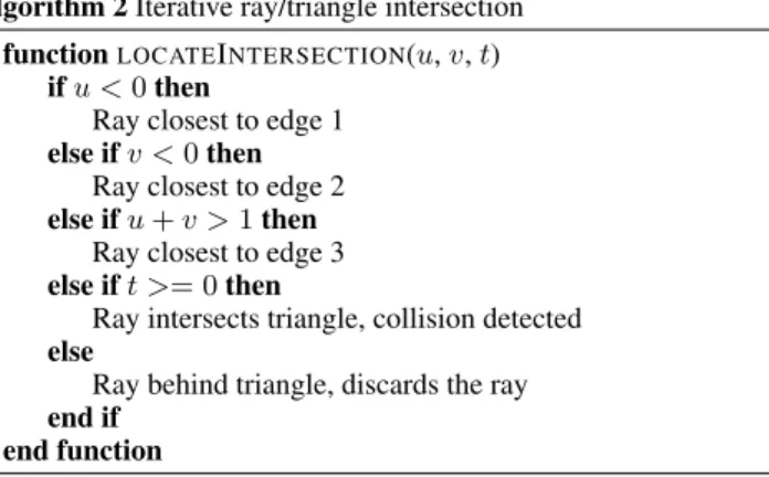
Algorithm 2 Iterative ray/triangle intersection functionLOCATEINTERSECTION(u, v, t)
if u <0 then
Ray closest to edge 1 else if v <0 then
Ray closest to edge 2 else if u+ v > 1 then
Ray closest to edge 3 else if t >= 0 then
Ray intersects triangle, collision detected else
Ray behind triangle, discards the ray end if
end function
3.3 Iterative Ray-Tracing Criterion
We need a criterion to know when we can use the iterative algorithm and when we need to use the non-iterative algorithm. The iterative algorithm can only be used on a pair when the relative displacement of the two objects since the last non-iterative iteration is small. This is because iterative ray/triangle-mesh intersection is only valid for small displacements. So, we need a relative displacement measure-ment and a threshold that indicates when the non-iterative algorithm must be used.
maxDis= ktni− tk + angle(qni, q) × maxRadius (2)
Equation 2 gives an upper bound to the maximum displacement, maxDis, between two points of the two objects where:
• (t, q) is the transformation from the reference frame of the first object of the pair to the second object. t is the vector that holds the translation and q is the quaternion that holds the rotation
• (tni, qni) is the transform between the two objects at the
mo-ment of the last non-iterative step
• angle(q1, q2) is the angle between the quaternions q1and q2.
• maxRadius is the largest radius of the two objects (ie: the radius of an object is the distance of the most off-centered vertex of the object).
ktni− tk denotes the displacement due to the pure translation.
angle(qni, q) × maxRadius is an upper bound of the
displace-ment due to the rotation. When maxDis exceeds a threshold displacementT hreshold we use the non-iterative algorithm, oth-erwise we use the iterative algorithm.
3.4 Concave and Missing Rays
In our iterative ray-tracing algorithm, when a ray goes through a concave area between two time steps it is trapped and lost (as shown on Figure 3). Accordingly, in theory we cannot use our algorithm on concave objects. Nevertheless, in our case we do not cast the ray on the entire objects but only in the interpenetrating surfaces. In the context of physics simulation, we try to minimize the interpenetra-tion throughout the simulainterpenetra-tion. This mean that the interpenetrating surfaces are small and the rays are short.
Even if the whole objects are concave, these small surfaces can be convex (see Figure 5), in such cases our algorithm is valid. In other cases we may lost some rays in the cavities but only if the displacement is too big. In our algorithm, the displacement is bound to a maximum which makes such cases not so frequent.
(a) (b)
Figure 5: Intersection volumes in a concave mesh can be convex. Two concave meshes are in collision (a), the intersecting surfaces are convex (b).
We can also lose some rays when vertices enter in collision between two standard steps. In such cases, the vertices will only be taken into account in the next standard step because, in the iterative steps, we only update previously colliding vertices.
In all cases where we can lose some rays, we can accept it as long as there is still enough rays to detect the collision and compute the physical response. Then, lost rays will be recovered in the next standard step.
3.5 Work Distribution for GPU
We propose to execute the iterative and standard ray tracing algo-rithms on GPU to improve performance. GPU works with highly parallelized execution, we have to send to the GPU the work as an array of threads of several indices. We propose to work with two indices. The first index iterates through the pairs of objects from the broad phase and each pair appears two times in opposite order. The second index iterates through the vertices of the first object of the pair, in each thread we cast the ray from the current vertex of the first object of the pair on the second object. This division on the work allows to parallelize the ray-tracing by executing one ray cast per thread.
4
Performance Comparison
This section presents our experimental scenes and the result of our tests.
Section 4.1 presents our experimental scenes. Section 4.2 presents the two standard ray-tracing algorithms we used with our iterative ray-tracing. Section 4.3 focuses on the performance of the GPU with or without our iterative ray-tracing algorithm.
4.1 Experimental Setup
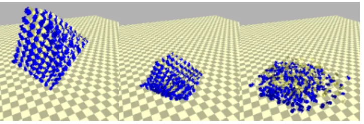
We have tested our IRTCD algorithm with two different scenes. The first experimental scene is an avalanche of 512 concave meshes on a planar ground (see Figure 6), each mesh is composed of 453 vertices and 902 triangles. When the objects hit the ground, ap-proximately 7300 pairs of objects are sent to the narrow-phase. In the second experimental scene, objects are continually added in the scene at 10 Hz from a moving source that follows a circle. Four dif-ferent concave meshes respectively composed of 902, 2130, 3456 and 3458 triangles are used. At the end 500 objects are present in the scene making a total count of approximately 1.2 million trian-gles in the scene and around 10,000 pairs of objects are sent to the narrow phase in the last steps. Both scenes work at 60 Hz.
Figure 6: Our first experimental scene.
4.2 Standard Ray-Tracing algorithms used
Our iterative tracing algorithm can work with any standard ray-tracing algorithms. We have tested two different standard ray-tracing algorithms. The objective is to compare the behavior of two algorithms with different properties with our iterative ray-tracing algorithm. This is motivated by the fact that naive algorithms that underperform on CPUs may outperform on GPUs due to their na-ture. The considered algorithms are:
Basic traversal: This algorithm does not use any acceleration structure, for each ray we iterate through each triangle. This method have a high complexity but is simple.
Stackless BVH traversal: This algorithm uses a bounding vol-ume hierarchy (BVH) as an accelerative ray-tracing structure [Wald et al. 2007] with a stackless traversal adapted for GPUs [Popov et al. 2007]. This algorithm is more computationally efficient but has in-creased memory usage due to auxiliary data structures.
4.3 Iterative Ray-Tracing Performances
We run our two experimental scenes with the two standard ray-tracing algorithms with and without our iterative ray-ray-tracing tech-nique on a Nvidia GTX 660 and focus on the GPU performance. In the first scene we can see three different phases in the simulation. Figure 7 shows the time spent on ray-tracing on the GPU at each simulation step.
Phase A: The objects are in free-fall and there is no collisions but the objects are close enough to be detected by the broad phase. Speedup when using our iterative algorithm is 3.7 for the basic algo-rithm and no speedup is observed for the stackless BVH traversal. Phase B: The objects hit the ground, it is a stressful situation as a lot of objects enter in collision simultaneously, it generates a peak in the computation time. Speedup when using our iterative algo-rithm is 1.3 for the basic algoalgo-rithm and 2.1 for the stackless BVH traversal.
Phase C: All the objects have fallen on the ground, the objects have smaller velocities. Speedup when using our iterative algorithm is 19.3 for the basic algorithm and 6.9 for the stackless BVH traversal. In the second scene, the computation time grows as the number of objects in the scene increases. At the end of the simulation, the iter-ative basic traversal algorithm have a29.1 average speedup against the non-iterative basic traversal algorithm, the iterative stackless BVH traversal algorithm have a18.8 average speedup against the non-iterative stackless BVH traversal algorithm.
The percentage of incorrectly detected collision pairs over the whole pairs tested in the narrow phase is in the worst case 1.7% in the first scene and 2.9% in the second scene. These errors are mainly false negative on pairs of object that are in collision with few vertices. These erroneous pairs are correctly detected after they moved of a distance of displacementT hreshold.
0 10 20 30 40 50 60 70 80 90 0 1 2 3 4 5 6 7 8 9 10 Co mp u ta ti o n ti me (ms ) Time in simulation (s) A B C
Hermann et al. with basic traversal Iterative with basic traversal Hermann et al. with stackless BVH traversal Iterative with stackless BVH traversal
Figure 7: Time spent executing ray-tracing in the first scene.
5
Conclusion and Future Work
In the context of collision detection, we presented IRTCD, a new It-erative Ray-Traced Collision Detection algorithm that exploits spa-tial and temporal coherency. Our algorithm uses an iterative ray-tracing algorithm that speedup any existing ray ray-tracing algorithm, experiments showed a speedup up to 19 times with a BVH traversal and 33 times with a basic ray traversal.
For future work, it would be interesting to extend our algorithm to deformable bodies. Indeed, we believe that IRTCD is also suitable for deformable bodies.
References
AVRIL, Q., GOURANTON, V., ANDARNALDI, B. 2011. Dy-namic adaptation of broad phase collision detection algorithms. In VR Innovation (ISVRI), 2011 IEEE International Symposium on, IEEE, 41–47.
HERMANN, E., FAURE, F., RAFFIN, B., ET AL. 2008. Ray-traced collision detection for deformable bodies. In 3rd Inter-national Conference on Computer Graphics Theory and Appli-cations, GRAPP 2008.
HUBBARD, P. 1993. Interactive collision detection. In Virtual Reality, 1993. Proceedings., IEEE 1993 Symposium on Research Frontiers in, IEEE, 24–31.
KOCKARA, S., HALIC, T., IQBAL, K., BAYRAK, C.,ANDROWE, R. 2007. Collision detection: A survey. In Systems, Man and Cy-bernetics, 2007. ISIC. IEEE International Conference on, IEEE, 4046–4051.
M ¨OLLER, T.,ANDTRUMBORE, B. 1997. Fast, minimum storage ray-triangle intersection. Journal of graphics tools 2, 1, 21–28. POPOV, S., G ¨UNTHER, J., SEIDEL, H.-P.,ANDSLUSALLEK, P.
2007. Stackless kd-tree traversal for high performance gpu ray tracing. In Computer Graphics Forum, vol. 26, Wiley Online Library, 415–424.
TESCHNER, M., KIMMERLE, S., HEIDELBERGER, B., ZACH -MANN, G., RAGHUPATHI, L., FUHRMANN, A., CANI, M., FAURE, F., MAGNENAT-THALMANN, N., STRASSER, W., ET AL. 2005. Collision detection for deformable objects. In Computer Graphics Forum, vol. 24, Wiley Online Library, 61– 81.
WALD, I., BOULOS, S., ANDSHIRLEY, P. 2007. Ray tracing deformable scenes using dynamic bounding volume hierarchies. ACM Transactions on Graphics (TOG) 26, 1, 6.