Bio-inspired swimming and flying – Vortex dynamics and fluid/structure interaction

HAL Id: tel-01098010

https://hal.archives-ouvertes.fr/tel-01098010

Submitted on 7 Jan 2015

HAL is a multi-disciplinary open access

archive for the deposit and dissemination of sci-entific research documents, whether they are pub-lished or not. The documents may come from teaching and research institutions in France or abroad, or from public or private research centers.

L’archive ouverte pluridisciplinaire HAL, est destinée au dépôt et à la diffusion de documents scientifiques de niveau recherche, publiés ou non, émanant des établissements d’enseignement et de recherche français ou étrangers, des laboratoires publics ou privés.

and fluid/structure interaction

Ramiro Godoy-Diana

To cite this version:

Ramiro Godoy-Diana. Bio-inspired swimming and flying – Vortex dynamics and fluid/structure in-teraction. Fluid mechanics [physics.class-ph]. Université Pierre et Marie Curie, 2014. �tel-01098010�

!"#$%&%'()&*+#,,#("#(,-./01!(023&*4#56(7(8 !"#"$%&"'()*+,%)-+./ !"#$%&'()%*+'(&,(*'-)%.-,/0&0+1(2'(3,&%*0-'*(&'(*,.4()*'-+05 40'67(2%.+('&&'(81*0+'('+(96"'&&'(21-0*'()1*'..0-'*:( 9-:5;,#(2(<=>(2$*(#%(2(3'5#??#$%(53''(*;$(*#3)&5#(1;??+$&52@ %&;$(A("')#,;BB#?#$%(&$%#3$2%&;$2,C(9-./01!(023&*4#56(?23D+#( 2&$*&(*2();,;$%'("#(";$$#3(+$#($;+)#,,#("E$2?&D+#(F,#(G*2+%( D+2$%&D+#HI(J(*;$(32E;$$#?#$%($2%&;$2,(#%(&$%#3$2%&;$2,C( 4;+K;+3*(&?B,2$%'#(2+(5L+3("#(023&*M(,-./01!(023&*4#56(B;+3*+&%( @ %&%+%("#*(/5&#$5#*(#%(4#56$;,;N&#*("#(023&*C !,(.%63'&&'(02'.+0+1(30-6'&&'(-",))60'(-6*(&'-(3,&'6*-(;%.2,5 <'.+,&'-(2'(&"#$%&'( 9#(*#3)&5#(1;??+$&52%&;$(A("')#,;BB#?#$%(&$%#3$2%&;$2,(2( @ %&;$2,#*M("-2553;O%3#(*2()&*&P&,&%'C( %32$*"&*5&B,&$2&3#*(B6E*&D+#Q56&?&#QP&;,;N&#I(#%("#(*#*()2,#+3*( F&$"'B#$"2$5#M(?;"#3$&%'M(*;P3&'%'M(&$$;)2%&;$M(B3'5&*&;$M( #R&N#$5#("#(D+2,&%'IC =*'<0'*(&,.4,4'(,3'$(&"'7+1*0'6*>(&"0<,4'(96'(&"#$%&'( 20;;6-'(+*,260+(&,(96,&0+1(26(20,&%46'(96"'&&'()*%)%-'(?(-'-( 20;;1*'.+-(),*+'.,0*'-:(( 9-./01!(023&*4#56(*#32("-2+%2$%(B,+*(5;$$+#(#%(3#5;$$+#("2$*( )&*+#,,#(3'+**&#(#*%(+$#(&$5&%2%&;$(J("'5;+)3&3(,-&$*%&%+%&;$M(+$( 255;?B2N$#?#$%()#3*(,2(5;$$2&**2$5#("#*(25%&)&%'*("#(,-:5;,#C( S(%32)#3*(#,,#M(,#*(25%#+3*("#(5#%%#(&$*%&%+%&;$(FB3;T#**#+3*M(56#3@ 56#+3*M(',U)#*M(2N#$%*I(";&)#$%(*#(*#$%&3(3#B3'*#$%'*(J(,#+3(K+*%#( )2,#+3(#%(*;+%#$+*("2$*(,#+3*(#TT;3%*(5;??+$*("#(T;3?2%&;$M( "-&$$;)2%&;$(#%("#(B3;K#5%&;$C(.,,#(";&%(,#*(T'"'3#3(#%(V%3#(*;+35#( 9-&$"&*B#$*2P,#(2"'D+2%&;$(#$%3#(,2(T;3?#(#%(,#(T;$"(#*%( ,-2P;+%&**#?#$%(5;6'3#$%("#*()2,#+3*(*+P%&,#*(D+#(B;3%#(,-./01!( 023&*4#56C(( !'-(<%+-5$&1-(2'(&,(.%63'&&'(02'.+0+1(30-6'&&' &$*%&%+%&;$ #R5#B%&;$ *;P3&'%' ','N2$5# B'3#$$&%' 5;6'3#$5# ?;"#3$&%' %32$*"&*5&B,&$23&%' B3'5&*&;$ *;+B,#**# "E$2?&*?# ;+)#3%+3# 2+(5;#+3("-+$(3'*#2+

Bio-inspired swimming and flying

Vortex dynamics and fluid/structure interaction

Ramiro Godoy-Diana

Chargé de recherches au CNRS

Document presented to obtain the Habilitation à Diriger des Recherches Université Pierre et Marie Curie

Jury presiding the HDR defense on December 16, 2014: Frédéric Boyer (École de Mines de Nantes, Rapporteur) Jérôme Casas (Université de Tours)

Matthias Heil (University of Manchester)

Maurice Rossi (Université Pierre et Marie Curie, Président du Jury) Lionel Schouveiler (Université Aix-Marseille, Rapporteur)

The present document, prepared in view of obtaining the Habilitation à diriger des recherches, reviews my main research subject at PMMH since 2006, which concerns the study of swimming and flying inspired by nature. Canonical examples of flapping flight and undulatory swim-ming are explored using simplified experimental models as a starting point. This allows for the discussion of some fundamental questions related to the physics of bio-inspired locomotion at “intermediate” Reynolds numbers. In particular, we address the strong fluid-structure interac-tions that arise in these problems, where we have focused on: simplified models of flapping foils in hydrodynamic tunnel experiments, especially in the dynamics of vorticity in the wake of an oscillating foil ; mechanical models of flapping flyers with flexible wings in a self-propelled configuration (in the spirit of the pioneer experiments of Etienne-Jules Marey), as well as novel experimental models of undulatory swimming.

Ramiro Godoy-Diana Paris, 2014

Physique et Mécanique des Milieux Hétérogènes (PMMH) UMR 7636 CNRS, ESPCI ParisTech, UPMC (Paris 6), UPD (Paris 7) 10 rue Vauquelin, 75005 Paris, France

"I’m as much in the dark as ever, though I’ve grown used in a sense to my obtuseness." Henry James The figure in the carpet

Avant-propos

Je présente ici une synthèse des travaux que j’ai développés au PMMH depuis 2006 sur la thématique de la propulsion “bioinspirée”. J’ai divisé ce mémoire en 4 chapitres principaux plus une introduction et un point de perspectives à la fin. Le tout sauf cet avant-propos est écrit en anglais, histoire de pouvoir partager ceci avec plus de monde... Les travaux décrits dans ces pages sont pour la plupart le fruit d’un travail en équipe. Je tente ici une brève histoire, mentionnant les collaborateurs principaux de ces dernières années. Par ordre plus ou moins chronologique et avec un grand merci à tout le monde.

Depuis mon recrutement au PMMH en 2006, mon objectif a été de développer une activité autour des problèmes de mécanique des fluides liés à la propulsion animale à “grand” nombre de Reynolds (les guillemets pour dire que grand peut être de l’ordre de 100 dans certains cas, ce qui ferait rire à un aérodynamicien). À l’époque la thématique était nouvelle pour moi et j’ai pu compter sur l’enthousiasme et bon conseil de José Eduardo Wesfreid, qui m’a encouragé à proposer ce sujet pour mon projet au CNRS (¡Gracias Jefe!). Je me suis donc naturellement intégré à l’équipe Instabilités, Contrôle et Turbulence, où j’ai pu aussi collaborer avec d’autres gens, en particulier avec Jean-Luc Aider qui venait d’arriver au laboratoire avec plusieurs projets autour du contrôle. Le début de la période qui concerne ce rapport corresponde aussi à l’arrivée de Catherine Marais [1], d’abord en stage de M2 et après doctorante, co-encadrée par J. E. Wesfreid et moi-même.

En 2008, après une recherche de collaborateurs potentiels dans le paysage français et eu-ropéen, nous avons mis en place un partenariat avec Jérôme Casas de l’Institut de recherches sur la biologie de l’insecte (IRBI) à l’Université de Tours et Laurent Jacquin du Département d’Aérodynamique Fondamentale de l’ONERA pour écrire un projet dédié à la “Physique des ailes battantes inspirées de l’insecte". Le projet, que j’ai coordonné, à reçu un financement de l’ANR dans le cadre du programme Blanc et nous a donné les moyens de faire mûrir petit à petit cette thématique. Le projet a été mené à terme avec succès, en changeant en cours de route plusieurs des objectifs initiaux, surtout pour suivre des nouvelles idées chez tous les partenaires. En ce qui concerne le travail au PMMH le point crucial a été de diriger notre attention aux problèmes d’interaction fluide-structure liés non seulement à la propulsion par ailes battantes mais aussi ouvrant la porte à l’étude d’autres systèmes de propulsion bio-inspirés comme par exemple la nage ondulatoire. Cette redéfinition des priorités a été le fruit d’une collaboration fondamentale de ces dernières années, celle avec Benjamin Thiria, Maître de conférences à l’Université Paris Diderot, qui est arrivé au PMMH en 2009 et avec qui nous avons peu à peu établi une petite équipe “Nage et Vol bio-inspirés” en dirigeant ensemble les projets de plusieurs étudiants. Nous avons encadrés notamment Sophie Ramananarivo (doctorante 2010-2014) [2] et Verónica Raspa (post-doc 2010-2013), dont les travaux constituent une partie importante des résultats commentés dans ce mémoire. Les thématiques se diversifient en ce moment, d’une part en ce qui concerne la locomotion bio-inspirée, en considérant des problèmes de dynamique collective (thèse de Intesaaf Ashraf, 2014-2017), de miniaturisation des nageurs (thématique menée par Miguel Piñeirua, post-doctorant 2014-2015 dans le groupe) ou des régimes transi-toires (thèse de Marion Segall sur la manoeuvre d’attaque des serpents en collaboration avec

J’en parlerai un peu dans la partie perspectives.

J’ai décidé de ne recueillir dans ce mémoire d’HDR que les travaux concernant la propulsion, en excluant ainsi une partie de mon activité de recherche de ces dernières années, qui concerne surtout ma collaboration avec José Eduardo Wesfreid sur les instabilités de sillage. Notamment, pour une partie de la thèse de Catherine Marais nous avons collaboré avec Dwight Barkley sur la réponse impulsionnelle du sillage d’un cylindre en régime sous-critique [3]. Puis, dans le cadre du Laboratoire Internationale Associé "Physique et Mécanique des Fluides" (France-Argentine), nous collaborons avec Juan D’Adamo sur les instabilités des sillages forcés [4; 5]. J’ai aussi gardé un oeil ouvert sur mes travaux précédant mon arrivée en France sur l’énergie de la houle [6], thématique qui restera d’actualité avec la perspective de nouveaux projets autour des énergies renouvelables.

Parmi d’autres collaborateurs que je n’ai pas cité ci-dessus, je voudrais notamment men-tionner D. Pradal (Mécanicien au PMMH qui a conçu et fabriqué plusieurs des montages ex-périmentaux dont on parlera dans la suite) ainsi que toute l’équipe de l’atelier du PMMH qui a un moment ou un autre ont participé au montage des manips. Aussi un grand merci à G. Bimbard (doctorante à l’IRBI), D. Kolomenskiy (Postdoctorant a l’U. de McGill), O. Marquet (Chercheur à l’ONERA-DAFE), R. Fernández-Prats et F. Huera-Huarte (Universitat Rovira i Virgili), G. Spedding (USC) et R. Zenit (UNAM) qui ont été des interlocuteurs importants à différents moments de ces dernières années.

Un mot sur les finances : en complément des ressources fournis par les organismes de tutelle du laboratoire PMMH (ESPCI, CNRS, UPMC et U Paris Diderot), les travaux décrits dans ce document ont été financés par l’Agence Nationale de la recherche (Project ANR-08-BLAN-0099, The physics of insect-inspired flapping wings, 2008-2012, PI : R. Godoy-Diana) et la Fondation EADS (Projet Fluids and elasticity for biomimetic propulsion, 2012-2014, PI : R. Godoy-Diana & B. Thiria). Pour avoir fait tourner toute cette machinerie, un chaleureux remer-ciement à l’équipe administratif du PMMH, Fred et Claudette aujourd’hui, Amina, Claudine,... hier. Ainsi qu’aux directeurs Philippe et Eduardo.

Et il ne me reste qu’un petit bout de page pour dire merci à nouveau ! Merci aux membres du jury qui vont lire les pages qui suivent, double merci aux rapporteurs qui devront écrire en retour. Merci à tous mes profs, étudiants, collègues et amis qui, au PMMH et ailleurs, ont partagé coeur et cerveau en sachant (ou peut être pas) que le retour sur investissement serait maigre. Un abrazo fuerte también a la familia, en especial a Sebas y Malena que me toleran en casa al grito de "¡Papá, ya no trabajes el fin de semana!"...

Contents

2 The flapping foil experiments 19 2.1 Transitions in the wake of a flapping foil . . . 19

2.1.1 Symmetry breaking of the reverse BvK wake . . . 22

2.1.2 Effect of the Reynolds number . . . 22

2.1.3 Foil flexibility . . . 23

2.2 Two parallel foils . . . 25

3 Le petit manège: a flapping flyer on a merry-go-round 29 3.1 A flexible-wing flyer in a self-propelled geometry . . . 29

3.2 Wing compliance . . . 31

3.3 Four-winged flyer . . . 36

4 Playing with Pieris rapae 39 4.1 Take-off force balance . . . 40

5 Undulatory swimming 43 5.1 Lighthill’s elongated body theory . . . 44

5.2 Elastic filament swimmer on a free surface . . . 45

5.3 Self-propelled swimming foils . . . 49

6 Perspectives 53 6.1 Insect flight . . . 53

6.2 Smaller swimmers and micro-swimmers . . . 54

6.3 Undulatory swimming . . . 56

6.4 Transient regimes . . . 58

6.5 Energy transfers in fluid-elasticity problems . . . 59

References lxi

Short bio lxix

1. Introduction

The following pages deal with various problems related to swimming and flying in na-ture. Aside from their evident biological relevance, the locomotion strategies found in nature in the flight of birds, bats and insects and the swimming of fish and marine mammals have long since served as inspiration for the development of artificial systems. The result of this pluri-disciplinary appeal is that literature abounds over an ample spectrum of approaches bounded by biology, physics and engineering. Not pretending to give an exhaustive review of these vast domains, we will start by pointing out here a few key issues, as well as some of the works that have been important in guiding our attempt to develop simplified models of flapping flyers and undulatory swimmers. Along the way we will hint on the questions that we have asked and, additionally, recall some of the customary analytical tools that have been proven useful in the quest for reasonable answers.

1.1 Flying

We will focus here in problems related to powered flapping flight, excluding thus some fas-cinating problems of aerial locomotion found in nature such as gliding or parachuting. From the biological point of view, the latter have not only been probable precursors of powered flight, but besides they constitute an ecologically advantageous strategy on their own. And it is needless to say that they have also inspired human-made devices —quoting Buzz Lightyear: “This is not fly-ing, this is falling with style!”. From the engineering perspective, gliding can be described using fixed-wing aerodynamics, something that does not work for flapping wings. In a conventional aerodynamic picture, the basic model considers an airfoil immersed in an externally imposed flow, which results in the production of lift and drag forces. Lift opposes the weight of the flying thing, while drag opposes thrust (see Fig. 1.1). The latter is thus provided independently of the wing, using a propeller, and determines the fundamental difference with flapping-powered flight,

Figure 1.2: Left: Wing of Reptile, Mammal, and Bird (From G. J. Romanes, 1892 [11]). Right: Dragonfly wings (Photo credit: P. Kratochvil).

where both lift and thrust are produced by the moving wing. This results in the appearance of a collection of unsteady mechanisms that are crucial components of the aerodynamic force bal-ance [see e.g. 7; 8]. As we will comment in more detail below, the dynamics of vortices around the wings plays a fundamental role concerning the mechanisms of unsteady force production.

Coming back to the realm of the living, four animal groups have evolved powered flight independently [9]. In addition to fuelling our intimate awe toward nature, this observation points our reflection to the concept defined by biologists as evolutionary convergence [10]: The fact that evolution has independently given rise in different non-related species to analogous structures that share form and function, as a result of their adaptation to similar environments. The reason for convergent evolution is the simple fact that a given trait gives a strong advantage to a species once it has appeared. And flight is definitely a particularly successful strategy for many reasons that range from local flight, such as escaping predators, catching prey or finding resources, to migration, where a whole population can move from one place to another, for instance following more favourable weather [9].

The wings of birds, bats and the now extinct pterosaur are all versions of a modified forelimb (see Fig. 1.2). In the case of insects on the contrary, wings come from a different body part altogether, as an independent structure attached to the upper part of the thorax, while the legs are attached to the bottom. Insects were also the first group to evolve powered flight, and they are the only winged invertebrates.

Insects cannot control the shape and motion of the wings within the wing itself as vertebrates do, since they do not have joints or muscles out in the wing. They have however a branching arrangement of veins that carry blood and air passages that can be used to control the stiffness of the wing [12]. These veins in certain insects work as springs and hinges permitting the wing

Bio-inspired swimming and flying structure to fold. Insect wings are thus compliant structures [13] and their elastic properties are certainly a fundamental issue of the mechanics of their flapping-based aerodynamic force production [14]. Part of the works reviewed here have been devoted to the study of such a fluid-elasticity problem, where the observation of insect wings in motion have served as inspiration for the development of laboratory models.

1.2 Swimming

We will not converse a lot here about the diverse diving and splashing feats achieved by humans, but a little about more professional swimmers such as fish. Using body undulations to produce a propulsive force is a widespread technique embraced by many different organ-isms over a wide range of scales [15]. Physically, as we will discuss further below, the size of the organism determines the type of forces at play in the dynamical balance of the locomotion problem: microscopic swimmers such as sperm or flagellated bacteria evolve in a dynamical en-vironment entirely governed by viscous friction [see e.g. 16], whereas in macroscopic organisms like aquatic vertebrates, friction forces are confined to a thin region surrounding the body —the boundary layer— and the production of a propulsive force relies also upon inertial momentum transfer to the fluid [see e.g. 17]. However, some features appear as crucial for every swimmer regardless of its size, such as the establishment of a propagative kinematics for the undulating wave that describes the body deformations. This question is at the core of the fluid-structure interaction problem of the artificial swimmers that appear in the following pages.

In what follows we will focus mostly on these inertial fish-like swimmers. The locomotion of fish or, more generally, of aquatic vertebrates has been extensively studied, in the first place from the biological perspective [18; 19], but also as a source of inspiration for engineering ap-plications [20; 21]. Different strategies to produce locomotive forces for swimming are found in nature (see Figure 1.3), which can be broadly separated in median and paired fin propul-sion (MPF) and body and caudal fin propulpropul-sion (BCF) [19; 22; 23]. On the latter category one can further distinguish the periodic steady regime observed during cruising, from transient ma-noeuvres such as sharp turns and fast starts. It has been shown that the main locomotor strategy observed in a given species is linked to the feeding problem: for instance, BCF steady swimmers feed from a widely dispersed source whereas species constantly performing transient fast-start and turn maneuvers rely on locally-abundant prey such as fish schools [22].

Aquatic vertebrates rely on muscular action distributed all along the body to prescribe the kinematics of any given swimming gait. And it has been shown that the wave of muscle ac-tivation travels down the fish much more rapidly than the wave of bending [24]. Speaking of bio-inspiration or biomimetism, the design elements of an artificial swimmer or flyer that one would like to copy from an animal can be envisaged at different levels. One approach is to reproduce a solution found in a real animal, say, an anguilliform swimmer, using sophisticated actuation and control to fine-tune a given body kinematics that has been "tested and approved" by nature to perform efficiently for a given task1_{. Impressive examples of this can be found in}

the literature, such as the robotic eel of EPFL’s Biorobotics Lab [25] or MIT’s robotuna [26]. 1. I had written here "...to be optimal for a given task" but I am evading the debate on optimality in the

Median and paired fin propulsion

Body and caudal fin propulsion Other

Figure 1.3: Swimming modes (modified from Webb, 1994 [23]).

In our work on bio-inspired swimmers a different approach has been pursued, one where the kinematics is not actively enforced, but is the passive outcome of the body elasticity of model swimmers where the actuation is localised: a strong fluid-structure interaction problem that has received considerable attention recently [see e.g. 27–29].

1.3 Fluid-structure interaction

In these problems of bio-inspired propulsion, it is thus the active motion of a structure (e.g. a wing or a fin) that produces a propulsive force by its interaction with the surrounding fluid (e.g. air or water). From the fluid dynamics point of view, where the moving structure determines the boundary conditions for the fluid motion, the problem will be strongly dependent on the types of forces driving the dynamical balance in the Navier-Stokes equations

∂u ∂t + (u · —)u = 1 r—p + n—2u + 1 r F, (1.1) — ·u = 0, (1.2)

Bio-inspired swimming and flying fluid of constant density r and constant kinematic viscosity n, described by its velocity and pressure fields,u and p, respectively, and subject to an external force F (the derivation of these equations from basic principles can be found in any hydrodynamics textbook, e.g. [30]). Writing U and L for the characteristic velocity and length scales of the problem in question one can rewrite these equations as

∂u

∂t + (u · —)u = —p + 1

Re—2u + F, (1.3)

— ·u = 0, (1.4)

where all variables are now dimensionless and Re = LU/n is the Reynolds number, which rules the aforementioned dynamical balance by settling the relative importance of inertial vs. viscous forces. The two limit cases in terms of Re have been widely studied: when Re 1 the vis-cous term is negligible and in practice the Euler equations for an ideal fluid are recovered, the pressure gradient being balanced by fluid inertia. In these high-Reynolds number flows, such as the flow around an airfoil, the effects of viscosity are confined to a thin boundary layer that matches over a small length scale the "outer" inviscid flow and the actual solid boundary, where the no-slip condition applies and the velocity of fluid particles must match the velocity of the boundary. In the other limit, for Re ⌧ 1, it is the viscous term that governs the dynamics. This limit, known as Stokes flow, describes for instance the propulsion of microscopic organisms using cilia or flagella. The Reynolds numbers relevant to animal swimming and flying cover a broad range (see Table 1.1), a lot of cases being “intermediate” with respect to the two lim-its mentioned above, those that conventional analytical methods are capable of handling [31]. Physical insight relevant to this intermediate range usually requires the correct modelling of the vortex dynamics detaching from the swimmer or flyer and considerable efforts in this sense have been widely documented in the literature [see e.g. 32–34, and references therein]. Control of vortices produced by flapping wings or fins to generate propulsive forces is the everyday task of birds, insects and swimming animals. And many studies of actual flapping extremities have been indeed driven by the need for a better understanding of this form of propulsion with the ultimate goal of enhancing man-made propulsive devices [see extensive reviews in 21; 35–38].

Table 1.1: Cruising Reynolds numbers

Bacterium ⇠ 10 5

Marine invertebrate larvae ⇠ 0.1 10

Drosophila ⇠ 102

Small fish (e.g. guppy) ⇠ 103

Dragonfly ⇠ 104

Tuna ⇠ 105

Fluid& Solid& Interface& Displacement,and, deforma1on,of,the,solid, Navier5Stokes, equa1ons, Kinema1c,condi1on, (Boundary,condi1ons,for,the,, fluid,problem), Fluid,forces,on,the,structure,

Reynolds Mass Elastoinertial Cauchy Elastoviscous

number ratio number number number

Re ⇠ f luid viscosityf luid inertia M⇠ solid massf luid mass Nei⇠solid elasticitysolid inertia Cy ⇠solid elasticityf luid inertia Sp ⇠solid elasticityf luid viscosity

Figure 1.4: Schematic diagram of the fluid and solid dynamics two-way coupling in a fluid-structure interaction problem (inspired from Doaré, 2010 [39]) and some usual dimensionless numbers.

Now consider the motion of the structure, i.e. the swimmer or flyer. While it constitutes the boundary condition for the fluid problem, its own dynamics is of course coupled to that of the surrounding fluid, establishing the two-way coupling described schematically in Fig. 1.4. The dominant features of the different branches in this full fluid-structure interaction problem picture are ruled by various non-dimensional parameters that weigh the relative importance of the different physical mechanisms at play. Some of these numbers are built solely from the comparison of different dynamical properties of either the fluid (e.g. the Reynolds number) or the solid physics, but others are intrinsically built from the comparison between the dynamics of the fluid and the structure. The table in Fig. 1.4 summarises some of the dimensionless numbers that can be built considering a model system where a slender flexible structure of characteristic length scale L, thickness h and bending rigidity B ⇠ Eh3_{(e.g. a beam or a plate) propels itself}

through a fluid of density r and viscosity µ at an average cruising speed U as the result of a harmonic oscillation of angular frequency w = 2p f and amplitude Aw imposed at one of its

ends. Such a simple model allows for the introduction of the key parameters that can be used to describe the locomotion problem of a flexible body in a fluid. We have already noted the dynamical regimes defined by the Reynolds number. Additionally, the mass ratio quantifies the effect of the surrounding fluid on the inertia term in the equation of motion of the structure, whereas Nei, Cy and Sp ponder, respectively, the solid inertia, the fluid loading (the dynamic

pressure) and the viscous forces with respect to the elasticity of the structure.

In the following chapters we will develop further these ideas for two particular cases, a flapping wing in air and a slender undulatory swimmer in water. The fluid-structure coupling arises in different manners in these two cases, although the basic solid model can be described

Bio-inspired swimming and flying

U

A

ω

φ

8;'O*'%$&:;,*O,D1;,FL(%%;'F,

f (Hz)

A

(cm

)

f (Hz)

v

(cm

.s

)

f (Hz)

U

(cm

.s

)

A

B

C

D

Forcing Fluid Swimmer

Amplitude of B Viscosity Flexibility Length

3Vpp (squares)

Water (filled markers)

mou (shades of blue) 4cm

mou 6cm dur (brown) 4cm • 9Vpp (circles) mou 3cm • mou 4cm • mou 5cm • mou 6cm • dur 4cm Water-Glycerol

(open markers) mou 4cm

tail to account for spatial damping, and the speed of the

traveling wave defined as v = f is computed using the

and the frequency

A

ω

a"

b"

Figure 1.5: Beam model for a flapping wing (a) or an undulatory swimmer (b). The characteristic velocity of the imposed actuation Aw and the resulting cruising velocity U are represented schemat-ically in both cases. Additionally indicated: for the flapping wing, the anglef that characterises the ratio of these two velocities; and for the undulatory swimmer, the phase velocity of the bending wave vj.

by the same Euler-Bernoulli beam (see Fig. 1.5), described in the small amplitude regime by [see e.g 40]:

µhtt+Bhxxxx+FNL= Ff /s+W (t) . (1.5)

Here h(x,t) is the lateral displacement of the beam (i.e. along a direction y perpendicular to the mean locomotion direction x), Ff /sis the effect of the fluid appearing as a force on the equation

for the dynamics of the structure, and W (t) is the imposed actuation, which for a flapping wing or fin can be usually modelled as above by a harmonic oscillation ⇠ Awsinwt.

But before considering the full fluid-structure interaction problem (that where the wing or fin is deformed under the action of the surrounding fluid), even the one-way problem where an effectively rigid but moving structure serves as boundary condition to the fluid problem can be non-trivial at these intermediate Reynolds numbers, in part because of the unsteadiness related to the dynamics of vorticity. We discuss in the following chapter some of the characteristic traits of the unsteady flows produced by a rigid structure oscillating in a fluid, focusing on a quasi-two-dimensional view of the vorticity dynamics in the wake of a very idealised flapping wing or fin.

1.4 Plan

This review is organised as follows: Chapter 2 is dedicated to our work using flapping foils in a hydrodynamic tunnel as a basic model to study vorticity dynamics in a simple propulsive wake. The chapter ends with a modified experimental setup with a self-propelled geometry where we explored the role of wake symmetry properties in the swimming performance. It is followed in Chapter 3 by the discussion of our flapping flyer models with flexible wings using a merry-go-round setup. Chapter 4 summarises our work with a real biological model, a Pierid butterfly, where we focused on a transient regime: the take-off maneuver. Our undulatory swimming studies are the subject of chapter 5 and, finally, the manuscript is closed in chapter 6 by a brief

account of current projects and perspectives. Chapters 2 to 5 open with a brief summary and a list of the corresponding references that are included in the selected publications appendix.

2. The flapping foil experiments

Figure 2.1: Fluorescein-dye visualisation of the vortex streets in the wake of a pitch-ing foil. Flow is from left to right. On top the reverse Bénard-von Kármán wake, on bottom an asymmetric wake. (Figure from [41])

Summary

This chapter reviews our work on propulsive wakes using experiments with flapping foils. The goal of these studies was to explore simple models that con-tain key dynamical elements, such as the creation and organisation of vorticity, that are crucial in every sys-tem involving flapping wings or fins as a means of producing propulsive forces. The first part is devoted to the study of the wake of a rigid flapping foil, in particular to the establishment of an ubiquitous fea-ture related to propulsive flapping motion, which is a vortex street with the sign of vorticity of each vortex reversed with respect to the typical Bénard-von Kár-mán (BvK) wake. We study the relationship between the evolution of the wake structure as a function of the flapping parameters and the drag-thrust transition [42], the symmetry breaking of the reverse BvK wake [41] and the effect of using a flexible foil instead of a rigid one [43]. We close this chapter opening a broader perspective on the problem of wake topology considering a two-foiled self-propelled swimmer [44].

Collaborators : C. Marais, V. Raspa, B. Thiria, J. L. Aider, J. E. Wesfreid References :

Godoy-Diana, Aider, Wesfreid Phys. Rev. E77, 016308 (2008). [42]

Godoy-Diana, Marais, Aider, Wesfreid J. Fluid Mech.622, 23-32 (2009). [41] Marais, Thiria, Wesfreid, Godoy-Diana J. Fluid Mech.710, 659-669 (2012). [43] Raspa, Godoy-Diana, Thiria J. Fluid Mech.729, 377-387 (2013). [44]

2.1 Transitions in the wake of a flapping foil

The primary goal of our work on this subject was to use one of the simplest flapping models, a pitching foil, with careful measurements on a hydrodynamic tunnel setup to explore the basic features of one of the landmarks of these bio-inspired propulsive wakes: the reverse Bénard-von Kármán (BvK) vortex street (see Figures 2.1 and 2.2).

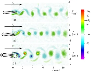
-1 0 1 2 y (cm ) -1 0 1 2 y (cm ) -2 -1 0 1 2 y (cm ) (a) (b) (c) d A U -40 -20 0 20 40 (s-1) wz 10 8 6 4 2 0 x (cm ) U U

Figure 2.2: Transition from the Bénard-von Kármán wake (top frame) to a reverse wake (bottom frame) seen in the vorticity field behind a flapping foil obtained from PIV measurements in a hydro-dynamic tunnel. The section of the foil is represented schematically. The Reynolds number based on the maximum width of the foil d was set to 255 (which corresponds to a chord-based Reynolds number of ⇠ 1200).

The indicator feature of this type of wake is a vortex street with the sign of vorticity of each vortex reversed with respect to the typical Bénard-von Kármán (BvK) vortex street behind a cylinder. Such reverse BvK vortex streets have not only been observed in the wakes of swimming fish [see e.g. 45; 46] but also studied in detail through laboratory experiments with flapping foils [47–54] and numerical simulations [50; 55–59]. In general, flapping-based propulsive systems, either natural or man-made, are often discussed in terms of the swept-amplitude-based Strouhal number [49; 60]:

StA=f A/U0, (2.1)

defined as the product of the flapping frequency f and amplitude A (the latter being a length scale similar to the width of the wake), divided by the cruising speed U0. Physically, the Strouhal

number represents the ratio of the flapping characteristic speed f A to the cruising velocity U and is thus related to the mechanical efficiency of the system. Biological swimmers and flyers are found to lie mostly in the range 0.2. StA. 0.4 [60; 61]. Another crucial parameter in these

problems is the aspect ratio of the flapping body, because it determines to what extent a quasi-two-dimensional (Q2D) view can capture the main elements needed for an adequate description of the real three-dimensional (3D) flow. In particular, in the case of a flapping body propelling itself in forward motion, at least two qualitatively different situations have been evidenced from flapping foil experiments and numerical simulations: high span-to-chord ratio foils produce the aforementioned reverse BvK vortex street [see e.g. 47; 49], where the most intense vortices are aligned with the foil span. A Q2D analysis accounts for the key dynamical features in this case where the mean flow has the form of a jet and results in a net propulsive force. As the

span-Bio-inspired swimming and flying St A D 0 0.1 0.2 0.3 0.4 0.5 0 0.5 1 1.5 2 St AD 0 0.1 0.2 0.3 0.4 0.5 0 0.5 1 1.5 2 0.6 0.6 0.3 0.3 0.3 0.3 0.3 0.6 0.6 _0.6

Figure 2.3: Left: Transitions in the wake of a flapping foil in the ADvs. St map for Re = 255 [from

41]. Experimental points are labeled as⇤: BvK wake; ⌅: aligned vortices; +: reverse BvK wake; M: deflected reverse BvK street resulting in an asymmetric wake. Solid line: transition between BvK and reverse BvK. Dashed line: transition between reverse BvK and the asymmetric regime. Typical vorticity fields are shown as inserts on each region. Right: Contours of a mean drag coefficient CD/CD0surface estimated using a momentum-balance approach (here CD0is the drag coefficient

for the non-flapping foil at zero angle of attack) [42]. The black line corresponds to CD=0 where

the estimated drag-thrust transition occurs. The shaded area represents the estimated error for the CD=0 curve due to sensitivity on the choice of the control volume. The blue line is the transition

from BvK to reverse BvK reproduced from the left panel. The dashed line corresponds to StA=0.3.

to-chord ratio decreases towards unity, 3D effects come into play and modify dramatically the structure of the wake. In this case a series of vortex loops (or horse-shoe vortices) are engendered from the vorticity shed from all sides of the flapping foil [see e.g. 54; 62; 63].

The experiments summarized here were performed with a 4:1 aspect ratio foil, which is high enough to produce Q2D regimes in the near wake. The foil section was chosen with a semi-circular leading edge that defines the maximum width of the foil, narrowing symmetrically to join the trailing edge along straight lines. The geometric simplicity and symmetry of this profile has motivated its use in further studies on the subject of flapping-based propulsion found in the literature [64–66]. Our experimental approach was inspired by the works on vorticity control in the cylinder wake forced by rotary oscillations conducted in previous studies at PMMH [67]. We showed that a two-parameter description that permits to vary independently the frequency and amplitude of the oscillatory motion is the optimum framework to fully characterize the quasi-two-dimensional regimes observed in the wake of a pitching foil. The transition from a BvK vortex street to the reverse BvK street characteristic of propulsive regimes (see Figure 2.2), as well as the symmetry breaking of the reverse BvK street reported in [41; 42] are summarized in the (St,AD)phase space shown in Figure 2.3 (left). The Strouhal number St = f D/U0and a

dimensionless amplitude AD=A/D have been defined using a fixed length scale (the foil width

D). Note that the product of these two parameters gives the flapping amplitude based Strouhal number from Eq. 2.1 that is often used. One of the main results of obtained form these

ex-periments is that the drag-thrust transition, which we estimated from mean flow measurements, does not coincide exactly with the inversion of the vortex street (see Figure 2.2, right), a fact that is usually assumed in the literature where "thrust-producing wake" is used interchangeably with "reverse Karman wake". In fact, a region in the (St,AD)plane exists where a reversed BvK

pattern can be observed in the wake of the flapping foil, but the relative thrust engendered by the flapping motion is not yet enough to overcome the total mean drag.

2.1.1 Symmetry breaking of the reverse BvK wake

The lateral deflection of the reverse BvK vortex street observed above a certain threshold in the forcing parameter space (above the green dashed line in Figure 2.3, left) was thoroughly scrutinised in these experiments, leading to the establishment of a symmetry breaking criterion [see 41, for details]. The latter is based on the qualitative observation that the deflection of the vortex street results from the formation of a dipolar structure from each couple of counter-rotating vortices shed on each flapping period. Above a certain threshold, the self-advection of the dipolar structure formed over one flapping period is strong enough to decouple from the subsequent vortex in the street and generate a deflection of the mean flow. This mechanism and symmetry breaking criterion have been subsequently verified by other studies [68–71]. The asymmetric wakes occurring in a region of the parameter space that overlaps the high-efficiency Strouhal number range used by flapping animals makes the precise definition of the symmetry-breaking threshold potentially important for the design of artificial flapping-based propulsors and their control.

2.1.2 Effect of the Reynolds number

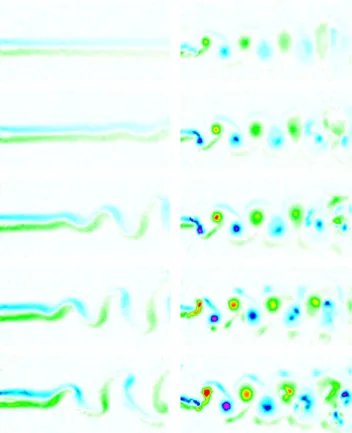
The Reynolds number dependance of the previous results was only barely mentioned in our initial work. An interesting point is that, although natural vortex shedding exists for the steady flap at these Reynolds numbers (the critical Reynolds number for the flap is approximately 140) even at zero-angle of incidence, no mode competition is observed in the strongly forced flapping regimes studied here. The flapping frequency used to define St is thus equivalent to the main vortex shedding frequency. However, even if for a fixed flapping configuration, i.e. fixed St and AD, one finds as expected a well defined wake structure, changing the Reynolds number does

change the intensity of the vortices, since these are built from the boundary layer vorticity on either side of the foil, which is evidently dependent on the Reynolds number. This is shown in Figure 2.4, where the vorticity field in the wake of the flap for a non-flapping case is compared to a case flapping at St = 0.25 and AD=1.42, a point in the parameter space where a clear reverse

BvK street is produced, for various Reynolds numbers. We remark for the non-flapping case (left column in figure 2.4) that small oscillations appear downstream of the flap at Re = 150 and a natural BvK vortex street is clearly established from the Re = 200 case. In the flapping case, increasing the Reynolds number for fixed St and ADproduces more intense vortices in the wake.

We note not only the increasing vorticity of the structures nearest to the symmetry plane, but also that of the filaments connecting opposite signed structures. Particularly in the cases of Re = 255 and 305, the filaments can be seen to concentrate producing two outer fringes of vortices with

Bio-inspired swimming and flying -40 -30 -20 -10 0 10 20 30 40 position mm 100 80 60 40 20 0 position mm -50 -40 -30 -20 -10 0 10 20 30 40 50 ROT-Z 1/s -40 -30 -20 -10 0 10 20 30 40 position mm 100 80 60 40 20 0 position mm -50 -40 -30 -20 -10 0 10 20 30 40 50 ROT-Z 1/s -40 -30 -20 -10 0 10 20 30 40 position mm 100 80 60 40 20 0 position mm -50 -40 -30 -20 -10 0 10 20 30 40 50 ROT-Z 1/s -40 -30 -20 -10 0 10 20 30 40 position mm 100 80 60 40 20 0 position mm -50 -40 -30 -20 -10 0 10 20 30 40 50 ROT-Z 1/s -40 -30 -20 -10 0 10 20 30 40 position mm 100 80 60 40 20 0 position mm -50 -40 -30 -20 -10 0 10 20 30 40 50 ROT-Z 1/s -40 -30 -20 -10 0 10 20 30 40 position mm 100 80 60 40 20 0 position mm -50 -40 -30 -20 -10 0 10 20 30 40 50 ROT-Z 1/s -40 -30 -20 -10 0 10 20 30 40 position mm 100 80 60 40 20 0 position mm -50 -40 -30 -20 -10 0 10 20 30 40 50 ROT-Z 1/s -40 -30 -20 -10 0 10 20 30 40 position mm 100 80 60 40 20 0 position mm -50 -40 -30 -20 -10 0 10 20 30 40 50 ROT-Z 1/s -40 -30 -20 -10 0 10 20 30 40 position mm 100 80 60 40 20 0 position mm -50 -40 -30 -20 -10 0 10 20 30 40 50 ROT-Z 1/s -40 -30 -20 -10 0 10 20 30 40 position mm 100 80 60 40 20 0 position mm -50 -40 -30 -20 -10 0 10 20 30 40 50 ROT-Z 1/s 1

Figure 2.4: Effect of the Reynolds number on the vorticity field in the wake of the foil. Left column: no flapping. Right column: flapping at St = 0.25 and A/D = 1.42. Values for Re are 100, 150, 200, 255, 305 from top to bottom. [Previously unpublished data]

local maxima weighing up to 30% in absolute value the vorticity of the inner array of vortices at the same horizontal position.

2.1.3 Foil flexibility

As mentioned in the introduction, a major part of our recent work has been devoted to ex-amining model flapping-based propulsion problems in cases where the elastic properties of the propulsive appendage come into play. In the following chapters we will review the problems that we have addressed in a full fluid-structure interaction framework. Before that, the case of the flapping foil in a hydrodynamic tunnel that we have been discussing in the previous sections permitted us to show how adding flexibility plays a strong dynamical role on the wake. We performed a detailed comparison of the vortex dynamics in the near wake of the flapping foil for two cases: the rigid foil (our benchmark case which is the foil of our previous studies), and a flexible foil with the same shape but made of a compliant material (Figure 2.5).

On the one hand, the effective amplitude obtained passively due to the deformation of the flexible foil while flapping (Fig. 2.5, right) leads to an increase in the propulsive force with respect to the case of the rigid foil [43]. On the other hand, the interaction of the shed vortices

Figure 2.5: Left: Photo of the flexible foil and schematic diagram. Right: Effective flapping ampli-tude Ae f f as a function of the Strouhal number StD= f D/U forq =5 (+), 7.5 (⇥), 10 (⇤) and

15 (?) (which means AD=0.7 (+), 1.1 (⇥), 1.4 (⇤) and 2.1 (?) for the rigid foil).

Figure 2.6: Top row: Isocontours of a mean drag coefficient CD/CD0 surface estimated using a

momentum-balance approach. The black contour corresponds to CD=0 where the estimated

drag-thrust transition occurs [see 42]. Bottom row: Cross-stream (y) profiles of the mean horizontal velocity on the downstream boundary of the control volume used for the thrust force estimation (solid lines) and corresponding rms (dashed lines) for a typical case (marked with a square symbol in the top plots) where the symmetry breaking is inhibited by the effect of foil flexibility. Insets: Snapshots of the mean < Ux>field showing the jet flow in the wake of the flapping foil.

Bio-inspired swimming and flying with the flexible structure inhibits the trigger of the symmetry breaking of the reverse Bénard-von Kármán wake, neutralising thus the deflection of the propulsive jet that has been widely reported in the literature (see Fig. 2.6 and [43]). The latter result evidences that wing compliance needs to be considered as a key parameter in the design of future flapping-propelled vehicles: since not only it is determinant for thrust and efficiency, but also as we show here because of its role in dictating the vortex dynamics that governs the stability properties of the wake.

2.2 Two parallel foils

We close this chapter discussing an experiment based on the same type of flapping foils actuated by a pitching oscillation that we have described above, but in a radically different

(c)! y x !u ! !ux !u y x (a)! 0 2 4 6 8 10 12 14 16 18 20 0 2 4 6 8 10 12 t / x/ c A mode! S mode! (b)! 0 0.5 1 1.5 2 2.5 3 3.5 −60 −40 −20 0 20 40 60 80 Foil 2 Foil 1 Δϕ/τ=0.5! 0 0.5 1 1.5 2 2.5 3 3.5 −60 −40 −20 0 20 40 60 80 Foil 1 Foil 1 Δϕ/τ=0! 0 0.5 1 1.5 2 2.5 3 3.5 −60 −40 −20 0 20 40 60 80 Foil 2 Foil 1 1

Figure 2.7: (a) Simplified schemes illustrating the topology and velocity fluctuations (˜u) of the considered wakes. Left: symmetric (S mode, jellyfish-like wake) where counter-rotating pairs of vortices are simultaneously shed into the wake. Right: asymmetric (A mode, fish-like wake) where counter-rotating vortices are alternatively shed into the wake by the flapping motion. (b) Swimmer’s reduced displacement (Dx/c) for the same distance between foils and forcing frequency in both flap-ping configurations. Substantially different displacements are achieved from the same momentum input. The driving curves are also shown, the phase lag (Df) being the only difference between both cases. [Figure from 44]

x/ c S mod e −4 −2 0 2 4 A mod e hux i [m / s] −0.2 −0.1 0 0.1 0.2 0.3 y / c x/ c −5 0 5 −4 −2 0 2 4 y / c −5 0 5 hp i po [P a ] −80 −60 −40 −20 0 x/ c −4 −2 0 2 4 h ˜uy i [m / s] 0 0.05 0.1 0.15 0.2 (a)! (b)! (c)! (d)! (e)! (f)!

1

Figure 2.8: (a, b) mean velocity measurements, (c, d) lateral fluctuations of the mean velocity and (e, f) pressure fields calculated from Eq.2.2 for a typical case of the two flapping configurations: Symmetric mode (Left column) and Asymmetric mode (right column).

setup. The idea came from the observation that, depending on the species, propulsive wakes found in nature can differ according to the spatial ordering of the main vortex structures. We used two foils placed in a side-by-side layout to analyse the role of the topology of the wake in the generation of propulsion by comparing two prototypical cases in a quasi-two-dimensional view. One configuration is jellyfish-like, with symmetric shedding of vortex pairs, and the other one is fish-like, with alternating shedding of counter-rotating vortices (see Figure 2.7). The setup was mounted in a water tank with a free surface in order to support the swimmer by means of an air-bearing rail outside of the water and achieve a self-propelled configuration [see 44, for details]. The crucial point to compare the role of vortex topology in the wake was to provide the same momentum input to produce the two different cases tested. This was carried out by tuning the imposed kinematics as shown in Figure 2.7, where it is also clear that the symmetric mode gives better swimming performance. PIV measurements showing the average velocity

Bio-inspired swimming and flying field in the direction of the propulsive jet huxi and the lateral fluctuations h ˜uyi are displayed in

Figure 2.8, together with a calculation of the average pressure field hpi derived from the lateral component of the mean Navier-Stokes equation in the turbulent approximation for developing jets (i.e. when the average lateral velocity huxi and the stream wise gradient of the Reynolds

stress are negligible), which reads [72]:

hpi po= r⌦˜u2y↵, (2.2)

pobeing the pressure away from the wake (y ! •), where⌦˜u2y↵is zero. These fields allowed

for the calculation of the average propulsive force per unit spanFp, which can be expressed as a

simple contribution from the momentumr hui and the pressure hpi [73; 74]: Fp= Z Ser hui hui·ndS Z SehpindS. (2.3) This very simple experiment allowed us also to identify the physical mechanism behind the better performance of the symmetric mode: a pressure effect related to the intensity of the velocity fluctuations in the near wake [44].

3. Le petit manège: a flapping flyer on a

merry-go-round

Figure 3.1: Top: Etienne-Jules Marey’s petit manège (from [75]). Bottom: PMMH’s petit manège

Summary

The work described in this chapter stems from two ideas that developed during our previous work with flapping foils in the hydrodynamic tunnel. We wanted: (1) a system in a self-propelled configu-ration, and (2) a simpler model to study the effect of wing flexibility on the performance of insect-like flapping wings. The result was the petit manège (Fig. 3.1, bottom) inspired by the classic setup conceived by Etienne-Jules Marey to record the kinematics of insect wings (Fig. 3.1, top). We have used this merry-go-round of a flapping device as an experi-mental platform for a thorough study of the effect of chord-wise flexibility on the performance of flapping wings [76; 77]. Additionally, a modified setup has also served to study the effect of forewing-hindwing interactions in a four-winged flyer.

Collaborators : S. Ramananarivo, M. Centeno, P. Jain, A. Weinreb, B. Thiria

Thiria, Godoy-Diana. Phys. Rev. E82, 015303R (2010). [76]

Ramananarivo, Godoy-Diana, Thiria. Proc. Natl. Acad. Sci. USA108 (15), 5964-5969 (2011). [77] Godoy-Diana, Jain, Centeno, Weinreb, Thiria. In Selected topics of computational and experimental fluid mechanics (Editors: Klapp et al.) Springer (2015). [78]

3.1 A flexible-wing flyer in a self-propelled geometry

A self-propelled geometry may sound like the evident choice to study a flapping-powered model, but experimentally it brings a certain amount of complications with respect to the usual

Figure 3.2: Schematic diagram of the flapping flyer in the merry-go-round setup during (a) cruising speed measurement and (b) thrust force measurement [From 76]. (c) Photo of the mechanical "in-sect" and (d) three instants of the flapping cycle superposed showing the bending wing from a frontal view (in white the leading edge, its tracking in blue; in green the tracking of the trailing edge). testing facilities (e.g. a wind tunnel or the hydrodynamic tunnel of the previous chapter) where an oncoming uniform flow is driven independently of the flapping motion.1 _{In particular, the}

actuation mechanism has to be mounted on the system that will move relative to the laboratory frame, and power needs to be supplied. The petit manège was designed with these requirements in mind, providing a setup (Figure 3.2) enabling measurements of the cruising speed, the thrust force, as well as the consumed power as functions of the imposed wing motion (flapping fre-quency and amplitude) and wing design. The design of the flyer itself also brought a set of constrains (additional to the choice of materials and actuation), since we wanted a system that performed reasonably well in terms of cruising speed but that remained simple enough to be tractable using basic models for the flexible wing deformation. We found inspiration for the final design of the wings from the literature on insect flight, in particular from Combes & Daniel [13], who showed for a wide variety of insect wings that span-wise flexural stiffness is 1–2 orders of magnitude larger than chord-wise flexural stiffness. We thus opted for wings with a rigid leading edge to focus on chord-wise deformation, and a semi-circular planform was used in order to minimise span-wise bending modes.

1. However, if one thinks of cruising flapping flight, the very fact of decoupling the flapping dynamics and the forward speed makes it difficult also to extrapolate any conclusions about flight performance to the case of a free-flying animal or machine.

Bio-inspired swimming and flying

3.2 Wing compliance

When considering a flexible wing in the dynamic regime, the forces acting to induce de-formation can come from both the fluid dynamic pressure acting on the surface of the wing and the inertial force due to the oscillating acceleration of the wing itself. A measure of the importance of these two bending forces can be given using a simplified model for the flapping wing as a plate of length L, mass surface density µs, and bending rigidity B (for a plate of

thickness h and Young?s modulus E, B ⇠ Eh3_{) whose leading edge is heaving sinusoidally with}

frequency w and amplitude A. The moment of the mean fluid pressure force scales then as Mf ⇠ rfu2fL3=rfw2A2L3, whererf is the fluid density and uf =Aw is the maximum flapping

velocity, whereas the moment of the inertia force scales as Mi ⇠ µsL3Aw2. The ratio of these

two moments Mi

M f is actually a mass ratio rµfsA, which is greater than 10 for all the wings tested in our experiments [76]. The main bending factor in this case is thus the inertia force, which will be counterbalanced by the elastic restoring force produced by the bent wing. This is consistent with the analysis by [79] who concluded for most wings moving in air that the feedback between fluid pressure stresses and the instantaneous shape of the wing is negligible with respect to the inertial-elastic mechanisms. Comparing the moment of the inertial force Mito that of the elastic

restoring force that scales as Me⇠ B, we defined the elasto-inertial number [76]

Nei= µsAw 2_L3 B = ✓ L Lb ◆3 , (3.1)

the latter form being expressed in terms of the bending length Lb= (B/µsAw2)1/3. Neimeasures

thus to what extent the inertial force due to the oscillating acceleration will be balanced by the elastic resistance to bending (analog definitions of this bending length arise in problems where other forces drive the bending, see [80; 81] for capillary and hydrodynamical forces, respectively). This definition determines for instance that for Nei⌧ 1 the wing is too rigid for

the inertia of the oscillating wing to have an observable effect, or in terms of the bending length, Lb L so that no deformation can be observed over the length scale L of the wing chord.

Physically, the form of the bending wing can be seen as a “shape factor” that redistributes the contribution of the aerodynamic forces in both directions –of the flapping motion normal to the wings FD1 and of the forward displacement– as sketched in Fig. 3.3. During the flapping

motion, the wings experience strong drag as they push fluid up and down during a stroke cycle. Because of the flexibility of the wing, the experienced drag scales on a length depending on Lb

[81–83], instead of L as it would for the rigid case. On the other hand, the change in shape induces a contribution of the aerodynamic pressure load in the forward direction that is also dependent on the wing bending.

Interestingly, the elasto-inertial number can also be expressed as a function of the ratio be-tween the forcing and relaxation frequencies times the non-dimensional forcing amplitude of the driving motion, which allows to express directly the bending rate as function of a non-1. FD is the drag force that opposes the flapping motion so that in the standard reference frame, where

the thrust force is in the direction of the cruising velocity, it is actually a fluctuating lift force, not to be confused with the drag that limits the cruising velocity.

Figure 3.3: Schematic diagram of the redistribution of aerodynamic forces by a bending plate model (top) with respect to a rigid plate (bottom). FTris the thrust force and FDrthe drag forces for a rigid

wing, respectively. [Figure from 76] dimensional oscillator forcing term:

Nei=Aw L ✓wf w0 ◆2 (3.2) an expression therefore useful to explore the nearness of the resonance which we have used to analyze the experimental data obtained with our flapping flyer [77].

The first two plots in figure 3.4 show the raw data for cruising speed and thrust force as a function of the flapping frequency for a series of wings of different thicknesses (and hence bending rigidities). The effect of wing flexibility is readily seen, the most flexible wings per-forming better, up to a certain frequency where the thrust force and thus also the cruising speed drop. All data can be analysed together using a non-dimensional representation for the thrust power given by the product of the dimensionless thrust force fT =FTL/B and cruising velocity

u = U/Aww. The bottom row plots in figure 3.4 show the dimensionless thrust and consumed

powers, pT =UFTL/BAww and pi=PiL/Bw, respectively, as a function of the reduced

fre-quency ¯wf = (wf/w0) = (NeiL/Aw)1/2. A clear maximum appears in the dimensionless aero-dynamic power. Notably, this maximum is located significantly below the structural resonant frequencywf =w0. We remark also that there is no sign of a resonant behaviour in the

con-sumed power curve (Fig. 3.4 (d)).

Observations of the wing deformation using high-speed video showed that it is reasonable to consider that the wings bend mostly over the first deformation mode, allowing for a forced-oscillator description where the oscillation of the leading edge is the forcing and that of the trailing edge is the response. Video tracking of the wing deformation was used as shown in Fig. 3.2(d) for the full parameter space, producing data for the non-dimensional amplitude a and phaseg of the response, i.e. of the trailing edge motion in the reference frame moving with the leading edge. Results are displayed in Fig. 3.5 where, in addition to all the experiments in a standard atmosphere, the experiments for the two most flexible wings were also performed

Bio-inspired swimming and flying 10 20 30 0 0.01 0.02 0.03 0.04 f (Hz) FT (N ) 10 15 20 25 30 35 0 1 2 3 f (Hz) U (m .s 1 ) 0 0.5 1 0 0.5 1 1.5 2 ¯f pt 0 0.5 1 0 200 400 600 800 ¯f pi (b) (c) (d) n e ar r i gi d c as e (a) wing thickness, h (mm) 0.050 0.078 0.130 0.175 0.250 0.360

mass per unit areaµs(kg.m 2) 4.50 10 2 10.63 10 2 17.67 10 2 24.12 10 2 34.92 10 2 47.95 10 2

rigidity B (N.m) 3.34.10 5 _1.83.10 4 _1.02.10 3 _2.26.10 3 _7.31.10 3 _14.00.10 3

relaxation frequency f0(Hz) 25.4 34.2 62.2 89.5 117.1 160.8

color label in figures blue red green yellow purple black

Figure 3.4: (a) Cruising speed, (b) thrust force and nondimensional (c) thrust (pT) and (d) input (pi)

powers as a function of ¯wf. The gray area represents the optimum region, the dashed line indicates

the location of the reduced natural frequency of the wing (linear resonance) [Figure from 77].

0 0.5 1 1.5 0 0.2 0.4 0.6 0.8 1 a ¯f 0.5 1 1.5 0.2 0.4 0.6 0.8 0 0.5 1 1.5 −pi/2 −pi/4 0 (ra d ) ¯f (a) (b)

Figure 3.5: Evolution of the non-dimensional amplitude a) and phase b) of the trailing edge wing response as a function of the reduced driving frequency for both flapping amplitudes Aw=0.8L and

Aw =0.5L (filled symbols correspond to measurements in air, open symbols in vacuum). Those

results are compared to nonlinear predictions from the model in Eq. 3.3 with (gray line) and without (black line) nonlinear air drag [Figure from 77].

in a vacuum chamber at 10 % of the ambient pressure. The latter permitted to test the role of the damping due to aerodynamic drag in the dynamics of the flexible wing. In order to analyse the previous results from a fluid-structure interaction point of view we used a non-linear beam model, i.e. Eq. 1.5 where FNLconsists of non-linear terms due to inertia and curvature and Ff /s

is a quadratic damping term to account for aerodynamic drag. Introducing a new dimensionless variable w(x,t) = (h(x,t) W (t))/L to describe the system in the reference frame of the leading edge the beam equation reads:

Linear beam z }| { w0000_{+ ¨w =} Curvature non-linearity z }| { (w0_w002_+w000_w02₎0 Inertial non-linearity z }| { 1 2 " w0Z x 1 ∂2 ∂t2 "_Z x 0 w 02_dx # dx #₀ Linear damping z }| { x ˙w Quadratic damping z }| { xnl| ˙w| ˙w Inertial forcing z }| { Aw L W¨ (3.3)

Keeping only the first mode of an expansion of the displacement as w(x,t) =•1Xp(t)Fp(x)

(whereFpare the non-dimensional linear modes for clamped-free beams) and using a classical

multiple scales method [see details in 77], the amplitude a and phaseg of the oscillation of the trailing edge can be obtained (lines in Fig. 3.5).

The main observations from Fig. 3.5 are the following: (1) the amplitude of the response increases rapidly with frequency, which is readily explained by the inertial forcing to the system (last term in Eq. 3.3), until it saturates because of the geometric limitation imposed by the finite chord length of the wing. Measurements in air and vacuum are approximately the same, in accordance with the hypothesis stated above that solid inertia is the main bending factor. (2) No clear resonance is observed around ¯wf =1 at these large-amplitude oscillations —only a barely

visible peak is observable when testing a lower flapping amplitude as shown in the insert in Fig. 3.5(a). A slight but rather broad peak can nonetheless be observed in the nearness ofw0/3

in the amplitude curve, which can be explained as a super-harmonic resonance consequence of the cubic nonlinearities in Eq. 3.3 [see 77]. (3) Concerning the phaseg, the present results recover the trend of what has been reported previously in the literature [84–87]: |g| increases monotonically with ¯wf. A remarkable point is that, contrary to what we have noted for the

amplitude a, there is a large difference in the evolution of the phaseg between the case in vacuum and that in air at atmospheric pressure: It is clearly observed thatg decreases more slowly in the low density environment within the whole range of flapping frequencies studied. From the beam model point of view, this shows that the quadratic damping term due to aerodynamic drag is responsible for the rapid phase lag observed when increasing the flapping frequency. Now, considering together the performance increase in the first part of the aerodynamic power curve pt( ¯wf)(Fig. 3.4(c)), and the corresponding increasing phase lag, supports the idea of a more

favourable repartition of the aerodynamic forces by the bent wing sketched in Fig. 3.3. Indeed, asg increases the wing experiences a larger bending at the maximal flapping velocity where the beneficial effect of bending the wing is most useful. Connecting the phase dynamics to the propulsive performance has been done in other configurations [85; 86] and it would mean that

Bio-inspired swimming and flying 0.4 0.6 0.8 1 1.2 0 0.5 1 1.5 ¯f / (I I ) (I )

Figure 3.6: Evolution of the two characteristic angles of the wing motion q and f as a function of the reduced driving frequency ¯wf. Two regimes can be distinguished: (I):f < q corresponding to the

performances increasing stage due to a useful phase lag. (II):f > q corresponding to the transition to under-performances due to a loss of the effective wing area. The optimum occurs therefore when f and q point at the same direction (best phase lag). [Figure from 77]

the thrust power should increase with the phase lag until the point where the wing experiences its largest bending at g = p/2, a point from which further increasing the phase lag would be counter-productive. However, while the previous argument can explain the initial trend of the performance curve in Fig. 3.4(c), it is clear that the maximum performance does not actually occurs at the expectedg = p/2, but relatively far below at around g ⇠ p/4.

Examining the wing deformation kinematics we showed that the optimum is actually ruled by an aerodynamic constrain: the previous argument for the theoretical optimal valueg = p/2 is only valid if the surrounding flow is totally attached to the wing (i.e. if separation occurs only at the trailing-edge). A measure of the susceptibility to separation from the kinematics is given by the ratio of the effective angle of attack at the leading edgef (equivalent to the advance ratio in propeller theory, see also [88, part III] and [89]) to the angle of the tangent to the wing at the trailing edgeq. A situation where q > f is strongly subjected to flow separation before the wing trailing edge. In this case the effective surface relative to the aerodynamic load can be expected to be drastically reduced leading to a loss of aerodynamic performance (see Figure 3.6).

Summarizing, the instantaneous wing shape is given by the two following ingredients: Iner-tia provokes the bending (gives the amplitude) and damping, by controlling the phase lag, allows this bending to be usefully exploited. From there, the aerodynamic mechanism described in Fig. 3.6 determines the limit of the beneficial effect of bending.

3.3 Four-winged flyer

From a biological point of view, the case of four-winged flyers capable of out-of-phase mo-tion between forewings and hindwings such as dragonflies is particularly interesting. In the words of [90]: “Dragonflies can hover, fly at high speed and maneuver skillfully in the air in order to defend their territory, feed on live prey and mate in tandem formation”. Forewing-hindwing phase-lag has been shown in hovering configurations to be determinant for flight per-formance [91]: optimal efficiencies have been found for out-of-phase beating whereas in-phase motion of forewings and hindwings has been shown to produce stronger force [92; 93]. The physical mechanisms behind these differences in performance have nonetheless not yet been completely elucidated, and open questions remain in particular when considering the role of wing elasticity. Wing deformation is important because it can passively modify the effective angle of attack of a flapping wing, determining thus its force production dynamics. We have used a modified version of our mechanical insect with two pairs of wings (Figure 3.7) to address these questions experimentally.

The two wings are driven by a single direct-current motor with a set of gears that allows to fix the phase difference between the forewings and the hindwings. All wings beat thus at the same frequency which was varied between 15 and 30 Hz. We have reduced the parameter space in the experiments reported here by fixing the physical characteristics of the flyer. Namely, the distance between the wings d, the stroke amplitudeq0 and the chord-wise flexural rigidity of the wings.

It should of course be noted that these parameters in the present tandem wing configuration, in particular the wing spacing d, should in general be analysed simultaneously with the forewing-hindwing phase lag [91; 94]. The motion of the wings is described using the angles of the forewing and hindwing leading edges in the flapping plane,qf wandqhw, respectively, as

qf w=q0sin(2p ft) and qhw=q0sin(2p ft j) , (3.4)

where f is the flapping frequency and the phase lagj is varied between 0 and 2p. For 0 < j < p the forewing is leading whereas forp < j < 2p it is the hindwing that leads. The Reynolds number Re = Uc/n based on the cruising speed and the chord length was in the range of 1000 to 4000.

The performance results are summarised in Fig. 3.8. In the first frame U is plotted in

Bio-inspired swimming and flying ϕ f (Hz ) U ( m s−1₎ 0 /4 /2 3 /4 10 15 20 25 30 35 ϕ f (Hz ) Pi( W ) 0 /4 /2 3 /4 10 15 20 25 30 35 η ϕ f (Hz ) 0 /4 /2 3 /4 10 15 20 25 30 35 0.5 1 1.5 2 1 2 3 4 5 6 7 8 9 0.01 0.02 0.03 0.04 0.05 0.06

Figure 3.8: Cruising speed, consumed power and efficiency (see text) as a function of the forewing-hindwing phase lag and the flapping frequency. Only the first half o the phase-lagj range where the forewing is leading was examined here.

coloured contours in a (j, f )-space for j 2 [0,p] and scanning the full range of flapping fre-quencies available experimentally. For all phase lags, a clear maximum of the attained cruising speed occurs always around 24Hz (the optimal frequency can be expected to be dictated by the elastic properties of the wings). The second plot in Fig. 3.8 shows the consumed power Pi in

the same parameter space. Here the main observation is that, while not surprisingly consumed power increases monotonically with increasing flapping frequency, phase lag plays an impor-tant role for energy expenditure, regardless of the flapping frequency. We use the two previous measurements to define the following expression of efficiency, considering that the aerodynamic thrust power is proportional to U3_{(velocity times thrust force, the latter being ⇠ U}2_):

h = 12rSU3

Pi (3.5)

where S is the effective wing surface. Other definitions of efficiency using purely dynamical parameters [e.g. 95] should give equivalent results to the expression 3.5 chosen here in terms of the measured consumed power Pi. It can be seen that the optimum in terms of efficiency

is shifted toward larger phase lags (around j ⇡ p/2) than the optimum in terms of maximum cruising speed [More details in 78].

4. Playing with Pieris rapae

Figure 4.1: Successive stages of the but-terfly take-off over half wingbeat period [From 96].

Summary

The present chapter reviews a project that emerged from the collaboration with Jérôme Casas’ group at IRBI in Tours. We used the small white cabbage but-terfly Pieris Rapae to study the take-off maneuver, which remains an elusive phase of insect flight rela-tively poorly explored compared to other maneuvers. Focusing on the first downstroke, we have addressed the different mechanisms involved in the force pro-duction during take-off from a force balance perspec-tive, in butterflies taking-off from the ground. In or-der to determine if the sole aerodynamic wing force could explain the observed motion of the insect, we have firstly compared a simple analytical model of the wings force to the acceleration of the insect’s cen-ter of mass estimated from video tracking of the wing and body motions. Secondly, the wing kinematics has also been used for numerical simulations of the aerodynamic flow field. Similar wing aerodynamic forces were obtained by the two methods. Both are however not sufficient, nor is the inclusion of the ground effect, to predict faithfully the body acceleration. We have to resort to the legs forces to obtain a fitting model. We show that the median and hind legs dis-play an active extension responsible for the initiation of the upward motion of the insect’s body, occurring before the onset of the wing downstroke. We estimate that legs generate, at various times, an upward force which can be much larger than all other forces applied to the insect’s body. The relative timing of leg and wing forces explain the large variability of trajectories observed during the maneuvers.

Collaborators : G. Bimbard1_{, D. Kolomenskiy, J. Casas}

Reference :

Bimbard, Kolomenskiy, Bouteleux, Casas, Godoy-Diana J. Exp. Biol.216, 3551-3563 (2013) [96].