HAL Id: hal-00477163
https://hal.archives-ouvertes.fr/hal-00477163
Submitted on 28 Apr 2010HAL is a multi-disciplinary open access
archive for the deposit and dissemination of sci-entific research documents, whether they are pub-lished or not. The documents may come from teaching and research institutions in France or abroad, or from public or private research centers.
L’archive ouverte pluridisciplinaire HAL, est destinée au dépôt et à la diffusion de documents scientifiques de niveau recherche, publiés ou non, émanant des établissements d’enseignement et de recherche français ou étrangers, des laboratoires publics ou privés.
Creation of a Transport Barrier for the E x B drift in
magnetized plasmas
Michel Vittot, Natalia Tronko
To cite this version:
Michel Vittot, Natalia Tronko. Creation of a Transport Barrier for the E x B drift in magnetized plasmas. Annals of the University of Craiova Physics AUC , Department of Physics, University of Craiova, 2009, 19, pp.59-72. �hal-00477163�
Creation of a Transport Barrier for the E × B drift
in magnetized plasmas
Natalia Tronko, Michel Vittot
Centre de Physique Théorique (CPT) - CNRS, Luminy - Case 907, 13288 Marseille cedex 09, France.
Unité Mixte de Recherche (UMR 6207) du CNRS, et des universités Aix-Marseille I, Aix-Marseille II et du Sud Toulon-Var.
Laboratoire affilié à la FRUMAM (FR 2291).
Laboratoire de Recherche Conventionné du CEA (DSM-06-35). E-mail: [email protected], [email protected]
Abstract
We modelize the chaotic dynamics of charged test-particles in a turbulent electric field, across the confining magnetic field in controlled thermonuclear fusion devices by a 112 degrees of freedom Hamiltonian dynamical system. The external electric field E = − ∇V is given by a some potential V and the magnetic field B is considered uniform. We prove that, by introducing a small additive control term to the external electric field, it is possible to create a transport barrier. The robustness of this control method is also numerically investigated.
1
Introduction
The confinement properties of high performance plasmas with magnetic confinement are governed by electromagnetic turbulence that develops in microscales [1]. In that frame-work various scenarios are explored to lower the turbulent transport and therefore improve the overall performance of a given device. The aim of such a research activity is two-fold. In this paper, we propose an alternative approach to transport barriers based on a macroscopic control of the E × B turbulence. Our theoretical study is based on a localized hamiltonian control method that is well suited for E ×B transport. In a previous approach [3], a more global scheme was proposed with a reduction of turbulent transport at each point of the phase space. In the present work, we derive an exact expression to govern a local control at a chosen position in phase space. In principle, such an approach allows one to generate the required transport barriers in the regions of interest without enforcing large modification of the confinement properties to achieve an ITB formation [2]. Although the application of such a precise control scheme remains to be assessed, our approach shows that local control transport barriers can be generated without requiring macroscopic changes of the plasma properties to trigger such barriers. The scope of the present work is the theoretical demonstration of the control scheme and consequently the possibility of generating transport barriers based on more specific control schemes than envisaged in present advanced scenarios.
Physics AUC, vol. 19, 59-72 (2009) PHYSICS AUC
In Section 2, we give the general description of our model and the physical motivations for our investigation. In Section 4, we explain the general method of localized control for Hamiltonian systems and we estimate the size of the control term. Section 5 is devoted to the numerical investigations of the control term, and we discuss its robustness and its energy cost. The last section 6 is devoted to conclusions and discussion.
2
Physical motivations and the
E
× B model
2.1
Physical motivations
Fusion plasma are sophisticated systems that combine the intrinsic complexity of neu-tral fluid turbulence and the self-consistent response of charged species, both electrons and ions, to magnetic fields. Regarding magnetic confinement in a tokamak, a large ex-ternal magnetic field and a first order induced magnetic field are organised to generate the so-called magnetic equilibrium of nested toroidal magnetic surfaces [4]. Experimen-tal strategies in advanced scenarios comprising Internal Transport Barriers are based on means to enforce these two control schemes. In both cases they aim at modifying macro-scopically the discharge conditions to fulfill locally the Chirikov criterion. It thus appears interesting to devise a control scheme based on a less intrusive action that would allow one to modify the chaotic transport locally by the choice of an appropriate electrostatic perturbation hence leading to a local transport barrier.
3
The
E
× B model
For fusion plasmas, the magnetic field B is slowly variable with respect to the inverse of the Larmor radius ρLi.e: ρL|∇ ln B| ¿ 1. This fact allows the separation of the motion of
a charged test particle into a slow motion (parallel to the lines of the magnetic field) and a fast motion (Larmor rotation). This fast motion is named gyromotion, around some gyrocenter. In first approximation the averaging of the gyromotion over the gyroangle gives the approximate trajectory of the charged particle. This averaging is the guiding-center approximation.
In this approximation, the equations of motion of a charged test particle in the presence of a strong uniform magnetic field B = Bˆz, (where ˆz is the unit vector in the z direction) and of an external time-dependent electric field E = − ∇V1 are:
d dT ⎛ ⎝ X Y ⎞ ⎠ = cE× B B2 = c B E(X, Y, T )× ˆz = c B ⎛ ⎝ −∂YV1(X, Y, T ) ∂XV1(X, Y, T ) ⎞ ⎠ (1)
where V1 is the electric potential. The spatial coordinates X and Y play the role of
canonically-conjugate variables and the electric potential V1(X, Y, T ) is the Hamiltonian
for the problem. Now the problem is placed into a parallelepipedic box with dimensions L× × (2π/ω), where L and are some characteristic lengths and ω is a characteristic frequency of our problem, X is locally a radial coordinate and Y is a poloidal coordinate.
A phenomenological model [5] is chosen for the potential: V1(X, Y, T ) = N X n,m=1 V0 cos χn,m (n2+ m2)3/2 (2)
where V0 is some amplitude of the potential,
χn,m≡ 2π L nX +
2π
mY + φn,m− ωT
ω is constant, for simplifying the numerical simulations and φn,mare some random phases (uniformly distributed).
We introduce the dimensionless variables
(x, y, t)≡ (2πX/L, 2πY/ , ωT ) (3) So the equations of motion (1) in these variables are:
d dt µ x y ¶ = µ −∂yV (x, y, t) ∂xV (x, y, t) ¶ (4)
where V = ε(V1/V0) is a dimensionless electric potential given by
V (x, y, t) = ε N X n,m=1 cos¡nx + my + φn,m− t ¢ (n2+ m2)3/2 (5) Here ε = 4π2(cV0/B)/(L ω) (6)
is the small dimensionless parameter of our problem. We perturb the model potential (5) in order to build a transport barrier. The system modeled by Eqs.(4) is a 11
2 degrees
of freedom system with a chaotic dynamics [5, 3]. The poloidal section of our modeled tokamak is a Poincaré section for this problem and the stroboscopic period will be chosen to be 2π, in term of the dimensionless variable t.
The particular choice (2) or (5) is not crucial and can be generalized. Generally, ω can be chosen depending on n, m. This would make the numerical computations more involved. In the following section, V is chosen completely arbitrary.
4
Localized control theory of hamiltonian systems
4.1
The control term
In this section we show how to construct a transport barrier for any electric potential V . The electric potential V (x, y, t) yields a non-autonomous Hamiltonian. We expand the two-dimensional phase space by including the canonically-conjugate variables (E,τ ),
H = H(E, x, y, τ ) = E + V (x, y, τ ) (7) The Hamiltonian of our system thus becomes autonomous. Here τ is a new variable whose dynamics is trivial: ˙τ = 1 i.e. τ = τ0+ t and E is the variable canonically conjugate to τ .
The Poisson bracket in the expanded phase space for any W = W (E, x, y, τ ) is given by the expression:
{W } ≡ (∂xW )∂y − (∂yW )∂x+ (∂EW )∂τ − (∂τW )∂E. (8)
Hence {W } is a linear (differential) operator acting on functions of (E, x, y, τ ). We call H0 = Ethe unperturbed Hamiltonian and V (x, y, τ ) its perturbation. We now implement
a perturbation theory for H0. The bracket (8) for the Hamiltonian H is
{H} = (∂xV )∂y− (∂yV )∂x+ ∂τ− (∂τV )∂E (9)
So the equations of motion in the expanded phase space are:
˙y ={H}y = ∂xV (x, y, τ ) (10)
˙x ={H}x = − ∂yV (x, y, τ ) (11)
˙
E ={H}E = − ∂τV (x, y, τ ) (12)
˙τ ={H}τ = 1 (13)
We want to construct a small modification F of the potential V such that e
H ≡ E + V (x, y, τ) + F (x, y, τ) ≡ E + eV (x, y, τ ) (14) has a barrier at some chosen position x = x0. So the control term
F = eV (x, y, τ )− V (x, y, τ) (15) must be much smaller than the perturbation (e.g., quadratic in V ). One of the possibilities is: e V ≡ V (x + ∂yf (y, τ ), y, τ ) (16) where f (y, τ )≡ Z τ 0 V (x0, y, t)dt
Indeed we have the following theorem:
Theorem 1 The Hamiltonian eH has a trajectory x = x0+ ∂yf (y, τ ) acting as a barrier
in phase space. Proof
Let the Hamiltonian bH ≡ exp({f}) ˜Hbe canonically related to eH. (Indeed the exponential of any Poisson bracket is a canonical transformation.) We show that bHhas a simple barrier at x = x0. We start with the computation of the bracket (8) for the function f . Since
f = f (y, τ ), the expression for this bracket contains only two terms,
{f} ≡ −f0∂x − ˙f ∂E (17)
where
f0 ≡ ∂yf and ˙f ≡ ∂τf (18)
which commute:
Now let us compute the coordinate transformation generated by exp({f}):
exp({f}) ≡ exp(−f0∂x) exp(− ˙f ∂E), (20)
where we used (19) to separate the two exponentials.
Using the fact that exp(b∂x)is the translation operator of the variable x by the quantity
b: [exp(b∂x)W ](x) = W (x + b), we obtain b H = e{f}H˜ ≡ e{f }E + e{f}V (x, y, τ )˜ =³E − ˙f´ + eV (x− f0, y, τ ) = E − V (x0, y, τ ) + V (x + f0− f0, y, τ ) = E− V (x0, y, τ ) + V (x, y, τ ) (21)
This Hamiltonian has a simple trajectory x = x0, E = E0, i.e. any initial data x = x0, y =
y0, E = E0, τ = τ0 evolves under the flow of bH into x = x0, y = yt, E = E0, τ = τ0+ tfor
some evolution yt that may be complicated, but not useful for our problem. Hamilton’s
equations for x and E are now
˙x ={ bH}x = ∂y[V (x0, y, τ )− V (x, y, τ)] (22)
˙
E ={ bH}E = ∂τ[V (x0, y, τ )− V (x, y, τ)] (23)
so that for x = x0, we find ˙x = 0 = ˙E. Then the union of all points (x, y, E, τ ) at
x = x0 E = E0: B0 = [ y,τ ,E0 ⎛ ⎜ ⎜ ⎝ x0 y E0 τ ⎞ ⎟ ⎟ ⎠ (24) is a 3-dimensional surface T2
× R, (T ≡ R/2πZ) preserved by the flow of bH in the 4-dimensional phase space. If an initial condition starts onB0, its evolution under the flow
exp(t{ ˆH}) will remain on B0.
So we can say that B0 act as a barrier for the Hamiltonian bH: the initial conditions
starting insideB0 can’t evolve outsideB0 and vice-versa.
To obtain the expression for a barrier B for eH we deform the barrier for bH via the transformation exp({f}). As
e
H = e−{f}Hb (25) and exp({f}) is a canonical transformation, we have
{ eH} = {e−{f}Hb} = e−{f}{ bH}e{f} (26) Now let us calculate the flow of eH:
et{ hH}= et(e−{f}{ eH}e{f}) = e−{f}et{ eH}e{f} (27) Indeed: et(e−{f}{ eH}e{f}) = ∞ X n=0 tn(e−{f}{ bH}e{f})n n! (28)
For instance when n = 2:
= t2e−{f}{ bH}2e{f } (29) and so et{ hH} = ∞ X n=0 tne−{f}{ bH}ne{f} n! = e −{f}et{ eH}e{f} (30)
As we have seen before:
e{f} ⎛ ⎜ ⎜ ⎝ x y E τ ⎞ ⎟ ⎟ ⎠ = ⎛ ⎜ ⎜ ⎝ x− f0 y E− ˙f τ ⎞ ⎟ ⎟ ⎠ and et{ eH} ⎛ ⎜ ⎜ ⎝ x0 y E0 τ ⎞ ⎟ ⎟ ⎠ = ⎛ ⎜ ⎜ ⎝ x0 yt E0 τ + t ⎞ ⎟ ⎟ ⎠ (31)
Multiplying (27) on the right by e−{f} we obtain:
et{ hH}e−{f} = e−{f}et{ eH} et{ hH}e−{f } ⎛ ⎜ ⎜ ⎝ x0 y E0 τ ⎞ ⎟ ⎟ ⎠ = et{ hH} ⎛ ⎜ ⎜ ⎝ x0+ f0(y, τ ) y E0+ ˙f (y, τ ) τ ⎞ ⎟ ⎟ ⎠ (32) and e−{f}et{ eH} ⎛ ⎜ ⎜ ⎝ x0 y E0 τ ⎞ ⎟ ⎟ ⎠ = e−{f} ⎛ ⎜ ⎜ ⎝ x0 yt E0 τ + t ⎞ ⎟ ⎟ ⎠ = ⎛ ⎜ ⎜ ⎝ x0+ f0(yt, τ + t) yt E0+ ˙f (yt, τ + t) τ + t ⎞ ⎟ ⎟ ⎠ (33)
So the flow exp(t{ eH}) preserves the set
B = [ y,τ ,E0 ⎛ ⎜ ⎜ ⎝ x0+ f0(y, τ ) y E0+ ˙f (y, τ ) τ ⎞ ⎟ ⎟ ⎠ (34)
B is a 3 dimensional invariant surface, topologically equivalent to T2
× R into the 4 dimensional phase space. B separates the phase space into 2 parts, and is a barrier between its interior and its exterior. B is given by the deformation exp({f}) of the simple barrierB0.
The section of this barrier on the sub space (x, y, t) is topologically equivalent to a torus T2.
This method of control has been successfully applied to a real machine: a traveling wave tube to reduce its chaos [6].
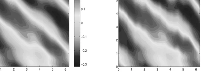
Figure 1: Uncontrolled and controlled potential for ε = 0.6, t = π4, x0 = 2
4.2
Properties of the control term
In this Section, we estimate the size and the regularity of the control term (15). Theorem 2 For the phenomenological potential (5) the control term (15) verifies:
kF k1 N, 1 N ≤ ε 2 N2e 3 4π (35)
if ε is small enough, i.e. if |ε| ≤ 2N e√π3/2 where N is the number of modes in the sum (5).
Proof The proof of this estimation is given in [7] and is based on rewriting
F = V (x + f0)− V (x) = Z 1
0
ds ∂xV (x + sf0, y, τ )f0(y, τ )
=O(V2) (36)
and then use Cauchy’s Theorem.
5
Numerical investigations for the control term
In this Section, we present the results of our numerical investigations for the control term F . The theoretical estimate presented in the previous section shows that its size is quadratic in the perturbation. Figure 1 shows the contour plot of V (x, y, t) and eV (x, y, t) ( eV = V + F) at some fixed time t, for example t = π4. One can see that the contours of both potentials are very similar. But the dynamics of the systems with V and ˜V are very different.
For all numerical simulations we choose the number of modes N = 25 in (5). In all plots the abscissa is x and the ordinate is y.
5.1
Phase portrait for the exact control term
To explore the effectiveness of the barrier, we plot (in Fig. 2) the phase portraits for the original system (without control term) and for the system with the exact control term
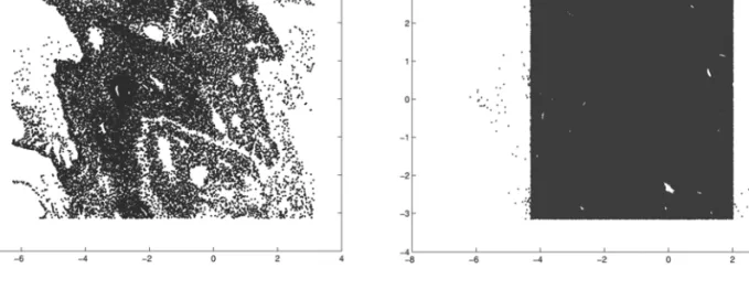
Figure 2: Phase portraits without control term and with the exact control term, for ε = 0.9, x0 = 2, Ntraj = 200
F. We choose the same initial conditions. The time of integration is T = 2000, the number of trajectories: Ntraj = 200 (number of initial conditions, all taken in the strip
−1 − π ≤ x ≤ −π; 0 ≤ y ≤ 2π) and the parameter ε = 0.9. We choose the barrier at position x0 = 2. And to get a Poincaré section, we plot the poloidal section when
t∈ 2πZ. Then we compare the number of trajectories passing through the barrier during this time of integration for each system. We eliminate the points after the crossing. For the uncontrolled system 68% of the initial conditions cross the barrier at x0 = 2 and for
the controlled system only 1% of the trajectories escape from the zone of confinement. The theory announces the existence of an exact barrier for the controlled system: these escaped trajectories (1%) are due to numerical errors in the integration.
One can observe that the barrier for the controlled system is a straight line. In fact this barrier moves, its expression depends on time:
x = x0+ f0(y, t) (37)
But when t ∈ 2πZ its oscillation around x = x0vanishes: f0(y, 2kπ) =
R2kπ
0 ∂yV (x0, y, t)dt =
0. This is what we see on this phase portrait. In fact we create 2 barriers at position x = x0, and x = x0− 2π (and also at x0+ 2nπ) because of the periodicity of the problem.
We note that the mixing increases inside the two barriers. The same phenomenon was also observed in the control of fluids [8], where the same method was applied.
5.2
Robustness of the barrier
In a real Tokamak, it is impossible to know an analytical expression for electric potential V . So we can’t implement the exact expression for F . Hence we need to test the robustness of the barrier by truncating the Fourier decomposition (for instance in time) of the controlled potential.
Fourier decomposition
Theorem 3 The potential (16) can be decomposed as eV =Pk∈ZVek, where
e Vk= ε N X n,m=1 Jk(nρ) (n2+ m2)3/2cos (η + kΘ + (k− 1)t) (38) with ηn,m(y) = nx + my + φn,m+ nεFc (39) Fc(y) = N X n,m=1 m cos(Kn,m,y) (n2 + m2)3/2 (40) Fs(y) = N X n,m=1 m sin(Kn,m,y) (n2 + m2)3/2 (41) Km,n,y = nx0+ my + φn,m (42)
and Jk is the Bessel’s function
Jk(nρ) =
1 π
Z π
0
cos (ku− nρ sin u) du (43)
Proof We rewrite explicitly the expression (16) for our phenomenological controlled potential eV (x, y, t): e V (x, y, t) = ε N X n,m=1 cos³n(x + f0(y, t)) + my + φn,m− t ´ (n2+ m2)3/2 (44) with f0(y, t) = ε N X n,m=1
m ³cos Kn,m,y − cos(Kn,m,y− t)
´
(n2+ m2)3/2 (45)
With the definition (40) and (41) we have:
f0(y, t) = ε(Fc(y) (1− cos t) − Fs(y) sin t) (46)
Let us introduce
ρ = ε(Fc2+ Fs2)1/2 (47) and Θ by
ρ sin Θ ≡ −εFc(y) ρ cos Θ≡ −εFs(y) (48)
so that e V = ε N X n,m=1 cos (η− t + nρ sin(Θ + t)) (n2+ m2)3/2 (49)
Using Bessel’s functions properties [9]
cos(ρ sin Θ) = X
k∈Z
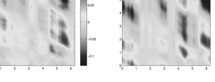
Figure 3: Exact Control Term and Truncated Control Term with ε = 0.6, t = π4 sin(ρ sin Θ) = X k∈Z Jk(ρ) sin kΘ (51) we get cos (η− t + nρ sin(Θ + t)) =X k∈Z Jk(nρ) cos (ξ) (52)
where ξ = η + kΘ + (k − 1)t, and we finally obtain (38). The theorem is proved. ¥ During numerical simulations we truncate the controlled potential by keeping only its first 3 temporal Fourier’s harmonics:
e Vtr= ε
N
X
n,m=1
A0+ A1cos t + B1sin t + A2cos 2t + B2sin 2t
(n2+ m2)3/2 (53) A0 =J0(nρ) cos(η + Θ) A1 =J0(nρ) cos η +J2(nρ) cos(η + 2Θ) B1 =J0(nρ) sin η− J2(nρ) sin(η + 2Θ) A2 =J3(nρ) cos(η + 3Θ)− J1(nρ) cos(η− Θ) B2 =−J3(nρ) sin(η + 3Θ)− J1(nρ) sin(η− Θ)
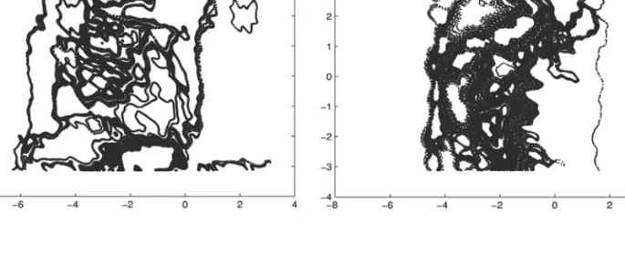
Figure 3 compares the two contour plots for the exact control term and the truncated control term (53). Figure4 compares the two phase portraits for the system without con-trol term and for the system with the above truncated concon-trol term (53). The computation of eVtr on some grid has been performed in Matlab and the numerical integration of the
trajectories was done in C.
One can see a barrier for the system with the truncated control term. As for the system with the exact control term we create two barriers at positions x = x0 and x = x0 − 2π
and the phenomenon of increasing the mixing inside the barriers persist.
5.3
Energetical cost
As we have seen before, the introduction of the control term into the system can reduce and even stop the diffusion of the particles through the barrier. Now we estimate the energy cost of the control term F and the truncated control term Ftr ≡ eVtr − V .
Figure 4: ε = 0.3, T = 2000, Ntraj = 50
Table 1: Squared ratios of the amplitudes of the control term and the uncontrolled electric potential ζex, ζtr; ratios of electric energy of the control term and the uncontrolled electic
potential ηex, ηtr; for the system with exact and truncated control term. ε ζex ζtr ηex ηtr 0.3 0.1105 0.1193 0.6297 0.1431 0.4 0.1466 0.1583 0.7145 0.2393 0.5 0.1822 0.1967 0.8161 0.3550 0.6 0.2345 0.2137 0.9336 0.4883 0.7 0.2518 0.2716 1.0657 0.6375 0.8 0.2858 0.3038 1.2119 0.8014 0.9 0.3191 0.3439 1.3722 0.9796 1.5 0.5052 0.5427 2.6247 2.3037
The average of any function W = W (x, y, τ ) is defined by the formula:
<|W | >= Z 2π 0 dx Z 2π 0 dy Z 2π 0 dt |W (x, y, t)| (54)
Now we calculate the ratio between the absolute value of the truncated control (electric potential) or the exact control and the uncontrolled electric potential:
ζex =<|F |2 > / <|V |2 > and
ζtr =<|Ftr|2 > / <|V |2 >
We also compute the ratio between the energy of the control electric field and the energy of the uncontrolled system in their exact and truncated version
ηex =<|∇F |2 > / <|∇V |2 > and
ηtr =<|∇Ftr|2 > / <|∇V |2 >
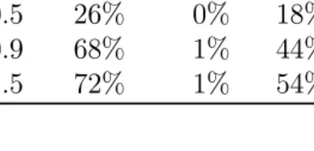
Table 2: Number of escaping particles without control term Nwithout, and for the system
with the exact control term Nexact and the truncated control term Ntr.
ε Nwithout Nexact Ntr
0.4 22% 0% 6% 0.5 26% 0% 18% 0.9 68% 1% 44% 1.5 72% 1% 54%
Table 3: Difference ∆N of the number of particles passing trough the barrier and differ-ence of relative electric energy ∆η for the controlled and uncontrolled system.
ε ∆N ∆η 0.3 8% 0.49 0.4 16% 0.47 0.5 8% 0.46 0.9 24% 0.39 1.5 18% 0.32
One can see that the truncated control term needs a smaller energy than the exact control term. In Table 2, we present the number of particles passing through the barrier in function of ε, after the same integration time.
Let ∆N = Nwithout− Ntr be the difference between the number of particles passing
through the barrier for the system without control and with the truncated control and ∆η = ηex− ηtr the difference between the relative electric energy for the system with the
exact control term and the system with the truncated control term. In Table 3 we present ∆N and ∆η for differents values of ε.
For ε below 0.2 the non controlled system is rather regular, there is no particles stream through the barrier, so we have no need to introduce the control electric field. For ε between 0.3 and 0.9 the truncated control field is quite efficient, it allows to drop the chaotic transport through the barrier by a factor 8% to 24% with respect to the uncontrolled system and it requires less energy than the exact control field. For ε greater than 1 the truncated control field is less efficient than the exact one, because the dynamics of the system is very chaotic. For example when ε = 1.5, there are 72% of the particles crossing the barrier for the uncontrolled system and 54% for the system with the truncated control field. At the same time the energetical cost of the truncated control field is above 70%of the exact one, which allows to stop the transport through the barrier. So for ε ≥ 1 we need to use the exact control field rather than the truncated one.
6
Discussion and Conclusion
In this article, we studied a possible improvement of the confinement properties of a magnetized fusion plasma. A transport barrier conception method is proposed as an alternative to presently achieved barriers such as the H-mode and the ITB scenarios. One can remark, that our method differs from an ITB construction. Indeed, in order to build-up a transport barrier, we do not require a hard modification of the system, such as a change in the q-profile. Rather, we propose a weak change of the system properties that allow a barrier to develop. However, our control scheme requires some knowledge and information relative to the turbulence at work, these having weak or no impact on the
ITB scenarios.
6.1
Main results
First of all we have proved that the local control theory gives the possibility to construct a transport barrier at any chosen position x = x0for any electric potential V (x, y, t). Indeed,
the proof given in section 4 does not depend on the model for the electric potential V . In Subsection 4.1, we give a rigorous estimate for the norm of the control term F , for some phenomenological model of the electric potential. The introduction of the exact control term into the system inhibits the particle transport through the barrier for any ε while the implementation of a truncated control term reduces the particle transport significantly for ε ∈ (0.3, 1.0).
6.2
Discussion, open questions
6.2.1 Comparison with the global control method
Let us now compare our approach with the global control method [3] which aims at globally reducing the transport in every point of the phase space. Our approach aims at implementing a transport barrier. However, one also observes a global modification of the dynamics since the mixing properties seem to increase away from the barriers.
Furthermore, in many cases, only the first few terms of the expansion of the global control term [3] can be computed explicitly. Here we have an explicit exact expression for the local control term.
6.2.2 Implementation of the control procedure
Let us now consider the implementation of our method to turbulent plasmas where the turbulent electric field is consistent with the particle transport. The theoretical proof of an hamiltonian control concept is developped provided the system properties at work are completely known. For example the analytic expression for the electric potential. This is impossible in a real system, since the measurements take place on a finite spatio-temporal grid. This has motivated our investigation of the truncated control term by reducing the actually used information on the system. As pointed out previously, one finds that this approach is ineffective for strong turbulence. Another issue is the evolution of the turbulent electric field following the appearance of a transport barrier. This issue would deserve a specific analysis and very likely updating the control term on a trasnport characteristic time scale. An alternative to such a process would be to use a retroactive Hamiltonian approach (a classical field theory) [10] and to develop the control theory in that framework.
Acknowledgements
We acknowledge very useful and encouraging discussions with Ph. Ghendrih, A. Brizard, C. Chandre, G. Ciraolo and M. Pettini. This work supported by the Euro-pean Communities under the contract of Association between EURATOM and CEA was carried out within the framework of the European Fusion Development Agreement. The views and opinions expressed herein do not necessarily reflect those of the European Commission.
References
[1] F. Wagner and U. Stroth, Plasma Phys. Contr. Fusion, 35, 1321 (1993). [2] E.J. Doyle et al., Nucl. Fus.,47 S18 (2007).
[3] G. Ciraolo, F. Briolle, C. Chandre, E. Floriani, R. Lima, M. Vittot, M. Pettini, Ch. Figarella, Ph. Ghendrih: “Control of Hamiltonian chaos as a possible tool to control anomalous transport in fusion plasmas”, Phys. Rev. E, 69, 056213 (2004). [4] J. Wesson, Tokamaks, Oxford University Press (2004).
[5] M. Pettini, A. Vulpiani, J. H. Misguich, M. De Leener, J. Orban, R. Balescu: “Chaotic diffusion across a magnetic field in a model of electrostatic turbulent plasma”, Phys. Rev. A 38, (1988) p 344-363.
[6] C. Chandre, G. Ciarolo, F. Doveil, R. Lima, A. Macor, M. Vittot: “Channelling chaos by building barriers”, Phys. Rev. Lett. 94, 074101 (2005).
[7] N. Tronko, M. Vittot: “Localized control theory for hamiltonian systems and its application to the chaotic transport of test particules in plasmas”. To appear in the proceedings of the “Joint Varenna - Lausanne International Workshop: Theory of Fusion Plasmas”, Varenna (August 2008)
[8] T. Benzekri, C. Chandre, X. Leoncini, R. Lima, M. Vittot: “Chaotic advection and targeted mixing”, Phys. Rev. Lett. 96, 124503 (2006).
[9] M. Abramowitz, I. A. Stegun, eds. Handbook of Mathematical Functions, (Dover, New York, 1965), p 361.
[10] I. Bialynicki-Birula, J. C. Hubbard, L. A. Turski: “Gauge-independent canonical formulation of relativistic plasma theory”, Physica A 128 (1984) p 509-519.