Decomposition of oil price Supply and demand shock in stock returns and economic performances

Decomposition of Oil Price Supply and Demand Shock in Stock Returns

and Economic Performances

By

Shuwen Wang

Master of Finance, 2021

SUBMITTED TO THE MIT SLOAN SCHOOL OF MANAGEMENT IN PARTIAL FULFILLMENT OF THE

REQUIREMENTS FOR THE DEGREE OF

MASTER OF FINANCE

AT THE

MASSACHUSETTS INSTITUTE OF TECHNOLOGY

FEBRUARY 2021

©2021 Shuwen Wang. All rights reserved.

The author hereby grants to MIT permission to reproduce

and to distribute publicly paper and electronic

copies of this thesis document in whole or in part

in any medium now known or hereafter created.

Signature of Author: _____________________________________________________________

MIT Sloan School of Management

December, 2020

Certified by: ___________________________________________________________________

Leonid Kogan

Nippon Telegraph & Telephone Professor of Management, Professor, Finance

Thesis Supervisor

Accepted by: ___________________________________________________________________

Heidi Pickett

Program Director, MIT Sloan Master of Finance Program

Decomposition of Oil Price Supply and Demand

Shock in Stock Returns and Economic

Performances

Shuwen Wang

Supervisor: Professor Leonid Kogan

Abstract

Oil price shock has always been serving as a ”mirror” reflecting the macroeconomic situation. However, it consists of di↵erent shocks from both demand side and supply side, and each side of the shock has di↵erent impacts on the economy. To extract more implications from oil price shocks, this thesis has several purposes. First, we proved the di↵erent lead-lag relationships between refined oil and crude oil during the shocks. Second, we utilized the properties of crack spread to define a new indicator that identify demand shock and supply shock in the total oil price change, and compared it with the traditional decomposition method, structural VAR model. Finally, we examined how much the decomposed shocks can explain the overall economic performances.

Contents

1 Introduction 3

2 Literature review: Oil price shock impacts 4 3 Lead-lag e↵ects in demand and supply shocks 5

4 Model Construction 7

4.1 A New Indicator: Theoretical Model . . . 8

4.2 Structural VAR model . . . 10

4.2.1 Identifying assumptions . . . 10

4.2.2 Decomposition System . . . 10

5 Empirical evidence 11 5.1 Data . . . 11

5.2 Identified main drivers by the Indicator . . . 12

5.3 Decomposed shocks by Structural VAR model . . . 13

5.4 Stock market . . . 14 5.4.1 Explanatory Models . . . 14 5.4.2 Robustness Testing . . . 16 5.5 Macroeconomic indicators . . . 17 5.5.1 Explanatory Models . . . 17 5.5.2 Robustness Testing . . . 19 6 Conclusion 21 7 References 22

1

Introduction

The futures price of crude oil plunged and went negative during the COVID-19 pandemic in March, 2020, meanwhile, we were experiencing a recession. As an important barometer reflecting the macroeconomic conditions, oil price shock has been a popular topic for a lot of researchers. Many researchers have worked on disentangling the oil price change into di↵erent shocks and discovered the main dominating shock driving the oil price(Kilian 2009). Their results have shown that di↵erent causes for the oil price change have di↵erent impacts on the economy.

A counter-intuitive empirical fact regarding oil price shock stated that the beta exposure of oil price change to the stock market index returns such as S&P500 or Dow Jones has been zero, contradicting the economic rationale that oil price has significant implications on the economic performances including stock market fluctuations. However, Robert C. Ready(2013) addressed this puzzle by orthogonal decomposition of demand and supply shocks. Positive impacts driven by demand shocks cancel out with the negative impacts from supply side, leading to a neutral exposure to the stock market. Furthermore, not only is the stock market the recipient of oil price shocks, but the heterogeneous impacts are reflected in the bond market as well as general economic indicators such as GDP growth, CPI, unemployment rate and so on (Demirer, et al, 2020). Due to this common decoupling e↵ect from demand and supply side, finding out the main drivers for the oil price change can serve as a reflection for the current or upcoming economic situations, which will be useful for policy-makers. For example, the negative oil futures prices plunged because of decreasing de-mand shocks, signaling a pessimistic and negative condition of the current econ-omy. If the price plunged because of increasing supply, then the result would be di↵erent. Therefore, this thesis aims at addressing this issue and providing a new indicator to identify the major drivers of the oil price change.

This thesis is structured as follows. The second section covers the general literature review for previous research. The third section proposes and proves the lead-lag relationship between refined oil and crude oil under di↵erent shocks. Then the fourth section provides theoretical framework and model for our new indicator, along with our structural VAR model. Next, we present the empirical test results, including the explanatory power for our stock sector index returns, and macroeconomic indicators. Other than that, we also look into how our models behave in di↵erent episodes such as global financial crisis and so on. Finally we make conclusions and look at some future research prospects.

2

Literature review: Oil price shock impacts

Oil price can fall or increase for di↵erent reasons. Since the oil demand shocks represent the variation of people’s needs for shipping, traveling and other activ-ities, if the crude oil price increases due to demand shock, it can be regarded as an optimistic sign for the economic conditions. Similarly, if the crude oil price increases due to shrinking supply, that means we’re experiencing a economic downturn. Not only does this rationale hold among the macroeconomic vari-ables, but it also holds for financial market and sovereign bonds, implying the patterns for the global financial market (Demirer, et al, 2020).

To decompose the shocks, researchers have been focusing on a classic and traditional method, structural VAR model. By identifying several assumptions regarding the covariates with shocks, Kilian(2009) disentangled not only demand shock and supply shock, but also some specific shocks related to the whole econ-omy. For example, he identified the increase of freight rates as a measure for global demand, and constructed an index for capturing real economic activities. After extracting these factors as indicators for economic activities, Kilian, Park (2009) also showed that di↵erent drivers of shocks lead to very di↵erent impact on the U.S. stock market. Unlike Kilian, Park (2009) and Kilian(2009) using

more macroeconomic factors , Robert C. Ready(2013) further validated the het-erogeneous property of oil shock drivers and their di↵erent impacts on the U.S. stock market by utilizing indicators such as the return of World-Integrated Oil Producers Index, and innovations of Crude Oil Volatility Index.

3

Lead-lag e↵ects in demand and supply shocks

We regard the spread between refined oil price and crude oil price as a start-ing point for the decomposition in this thesis. Intuitively speakstart-ing, since the demand shock reflects directly and immediately in refined oil such as heating oil, gasoline and so on, the price of refined oil should react first. Then this ”second-handed” demand shock will transfer to crude oil price, forming a lead-lag relationship between refined oil and crude oil. Similarly, when supply shock shows up, since crude oil is more directly exposed to it, this shock will first reflect in the price change of crude oil, and then as the refiners reproduce the oil into heating oil or gasoline, the supply shock will then be absorbed by refined oil price. Hence, the lead-lag relationship holds for both demand shock and supply shock (Kogan, Ahn, 2012).

To verify the existence of lead-lag e↵ect, we used Granger Causality test to examine it during specific periods when demand and supply shock hit. We picked several significant periods where demand shock hits(listed in Table 1).

Granger Causality Test Result

Period Lead-lag e↵ect p-value U.S.-led invasion of Iraq,

2003

Crude oil leading heating oil

0.0074 Pre-Global Financial

Cri-sis, 2006-2008

Heating oil leading crude oil

0.0032 Global Financial Crisis,

2008-2009

Heating oil leading crude oil

0.0001 COVID-19 Pandemic,

2020

Crude oil leading heating oil

0.0032 Table 1: History episodes of di↵erent oil shocks

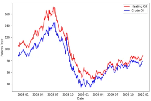
Figure 1: Heating Oil vs Crude Oil Futures price in Global Financial Crisis In March, 2003, U.S. armies invaded Iraq. As a main oil producer and ex-porter in the world, this caused declining oil supply in U.S. The oil production in U.S. decreased 4.5% in April, 2003, a month after the invasion in March. This negative supply shock is consistent with our significant Granger Causality test in that period, namely, crude oil price was leading the heating oil price in

a significant way.

Figure 1 depicts the moving patterns of both heating oil futures price and crude oil futures price. It’s clear that before July, 2008, the economic bubbles remained, which causes unusual rising demand. After the bubble burst, the global financial crisis came, reverting the previous positive demand shocks to negative demand shocks and supply shocks. During the post-global financial crisis period in 2009, economy started to recover and demand shocks became positive again. The above recognized shocks were correctly captured by the Granger Causality test between futures prices of heating oil and crude oil.

4

Model Construction

As we just proved in the previous section, in periods where demand shock is the main driver of the oil price fluctuation, refined oil price reacted first and crude oil price responds later. In periods where supply shock outweighs demand shock, crude oil moves earlier than refined oil. Crack spread, the spread between refined oil price and crude oil price serves as an ideal intermediate measure for identification of di↵erent shocks. We develop a new idea for identify the main drivers using crack spread.

When there is a positive demand shock, refined oil price moves first leading the crude oil price, causing the crack spread to widen. Furthermore, this in-creasing demand will also lead to rising crude oil prices. In this case, the crack spread change and the crude oil price change have the same sign. For negative demand shocks, crack spread will shrink, along with declining crude oil price. Signs of crack spread change and crude oil price change are consistent as well.

However, if there is a positive supply shock, crude oil price declines first and then leads the refined oil price to fall. The crack spread will get larger in this case. Hence the multiplication of crack spread change and crude oil price turns

negative. Same thing applies for negative supply shock.

We can conclude that if demand shock dominates, the multiplication of crack spread change and crude oil price change remains positive because they have the same sign, no matter whether positive or negative the shock is. If supply shock dominates, the crack spread change and crude oil price change share opposite signs, no matter positive or negative supply shock, so the multiplication of these two is negative. This identifier at time t is defined as

It= Ptcrd CrackSpread (1)

4.1

A New Indicator: Theoretical Model

Price change of crude oil at time t is denoted as Pcrd

t , where refined oil price

change is written as Ptref. We assume that:

1. At time t, all oil price changes can be captured by demand shock ✏d,t, supply

shock ✏s,tand a systematic risk shock ⌘t.

2. All three shocks follow normal distributions,

✏d,t ⇠ N(0, d2)

✏s,t⇠ N(0, s2)

⌘t⇠ N(0, 2)

Any two shocks are orthogonal to each other and time-serially independent, namely,

Cov(✏d,t, ✏s,t) = 0 (2)

Cov(✏d,t, ⌘t) = 0 (3)

Cov(✏s,t, ⌘t) = 0 (4)

Due to the lead-lag e↵ect of crude oil price and refined oil price during demand shock and supply shock, we can formulate the price changes as follows:

Ptcrd = d✏d,t 1+ s✏s,t+ ⌘t

Ptref = d✏d,t+ s✏s,t 1+ ⌘t

Then the change of crack spread satisfies:

Ptref Ptcrd = (✏d,t ✏d,t 1) (✏s,t ✏s,t 1) (5)

, which can be written as

CrackSpread = ✏d,t ✏s,t (6)

The change of crude oil price can be shown as

crdt = ✏d,t+ ✏s,t (7)

. We can define a new indicator as

It= crdt CrackSpread (8)

equivalently, because both shocks are time-serially independent and orthog-onal to each other, we have

If this indicator is larger than zero, then the magnitude of demand shock dom-inates over supply shock. If it’s negative, then supply shock explains more for the price change. Hence, this indicator can be applied to identify the major driver for supply shock or demand shock.

After we recognize the main driver for each time period theoretically, we label that period as demand shock or supply shock. Then we use the spot price change of refined oil as demand shock, and we use the negative spot price change of crude oil as supply shock.

4.2

Structural VAR model

As a classic method to solve oil price shock problems, here we look into structural VAR model. Built upon the work of Kilian(2009) and Robert C. Ready(2013), we constructed structural shocks by recognizing correct respondents. Now we identify the corresponding respondents according to our calculated main drivers. 4.2.1 Identifying assumptions

We want to decompose three shocks of oil: demand shock, supply shock and risk shock. Here we assume the decomposition system to be triangular. First, when the oil demand increases, oil suppliers will increase their production ac-cordingly. We assume that oil production change can capture the oil demand shock. Second, when oil supply shock comes in together with oil demand shock, they show up in the world integrated oil producers index return. To include the common systematic risks in oil price, we also consider crude oil volatility index as a good measure. Therefore, we built our system as follows.

4.2.2 Decomposition System

Let prodOP EC _{denote OPEC’s oil production change, R}prod

t denote the

re-turn of world integrated oil producers index, and ⌘OV X

t is the detrended

oil demand shock, oil supply shock and systematic risk shock respectively. 0 B B B @ prodOP EC Rprodt ⌘OV X 1 C C C A= 0 B B B @ a11 0 0 a21 a22 0 a31 a32 a33 1 C C C A 0 B B B @ ✏demand ✏supply ✏risk 1 C C C A (10) The structural VAR model can be represented as follows:

A0zt= 12

X

i=1

Ai+ ✏t. (11)

Here ✏trepresents the serially independent structural shocks. Define et as the

reduced-form VAR innovations such that et= A01✏t. This model imposes that

et= 0 B B B @ prodOP EC Rprodt ⌘OV X t 1 C C C A= 0 B B B @ a11 0 0 a21 a22 0 a31 a32 a33 1 C C C A 0 B B B @ ✏demand ✏supply ✏risk 1 C C C A (12)

This model assumes that OPEC oil production change doesn’t react to oil supply shock, but only reacts to the oil demand shock. World integrated oil producers index return can capture both demand and supply shock, but not move with other systematic risk shock. However, the OVX innovations can delineate all the shocks.

5

Empirical evidence

In this section we’re going to show the empirical test results of our new indicator identification and the structural VAR model.

5.1

Data

For both spot price and futures price data, we are using data from U.S. Energy Information Administration(E.I.A). For the data of macroeconomic indicators,

our data source is the open database from FRED. Market indices and sector indices data are cited from FactSet database. Our data spans from 1980/01/01 to 2020/05/27.

Summary of data source

Data Source

Crude oil, heating oil and gasoline (spot price)

U.S. EIA Database Crude oil, heating oil and

gasoline (futures price)

U.S. EIA Database GDP, CPI, Core Inflation,

Nonfarm payroll, Unem-ployment rate, 10-year Treasury rate

FRED Economics data

Market indices(Nasdaq, Dow Jones, etc), S&P sector indices(Airline, transportation, utility, etc)

FactSet

Table 2: Data Source Description

5.2

Identified main drivers by the Indicator

By utilizing the new crack-spread indicator It, we recognize the main driver

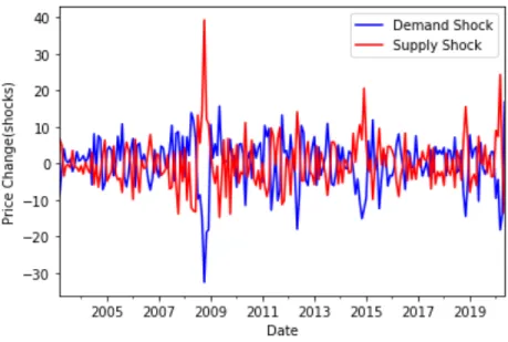
of shocks during that time period, and label that period as demand or supply. Then the corresponding refined oil price change can represent demand shock, while the corresponding crude oil price change serves as supply shock. The following Figure 2 depicts the monthly aggregated patters of both identified shocks.

Figure 2: Main drivers identified by the indicator

5.3

Decomposed shocks by Structural VAR model

After implementing the structural VAR model, we extracted two time-series patterns for demand shock and supply shock. Figure 3 captures the fluctuating extracted patterns.

5.4

Stock market

After we decompose the shocks from the total oil price change, we want to examine how each side of the shock a↵ects di↵erent sectors in the stock mar-ket. For example, we’ll check its influences on various industries like airline, transportation, utility, technology, etc.

5.4.1 Explanatory Models

Let Rt depicts the sector s index return. Here we consider various sectors

such as transportation, airline, utility, etc. ✏I demandt , ✏I supplyt are the shocks

identified by our indicator for demand side and supply side. ✏S demandt , ✏S supplyt

are demand and supply shocks extracted by our structural VAR model. We want to see how much these shock can explain for the total index return variation.

Rst= ↵ + 1✏I demandt + 2✏I supplyt + ✏t (13)

Since the structural VAR decomposed shocks include demand, supply and risk, to make it comparable with the power of our crack-spread indicator, here we eliminate risk shock to just look at its pure demand and supply shocks

Rs

t = ↵ + 1✏S demandt + 2✏S supplyt + ✏t (14)

Sector returns vs. Indicator-shocks Sectors Coef. ✏I demandt Coef. ✏

I supply t R2 Airline -0.0004 -0.0015 0.9% Transportation 0.0007 0.0022⇤⇤ _9.6% Energy 0.0010⇤ _-0.0055⇤⇤⇤ _40.6% Utility 0.0003 -0.0010⇤ _5.6% Refiners -0.0027⇤⇤⇤ _0.0027⇤⇤⇤ _29.6% Technology 0.001⇤⇤ _-0.0017⇤⇤⇤ _16.0% Material 0.0009⇤ -0.0029⇤⇤⇤ 21.2% S&P 500 0.0007⇤ -0.0018⇤⇤⇤ 18.8% Dow Jones 0.0005 -0.0017⇤⇤⇤ 14.8%

Table 3: Indicator-identified shocks vs. Stock market

Sector returns vs. Structural-shocks Sectors Coef.✏S demandt Coef.✏S supplyt R2

Airline -0.0002 0.0064⇤⇤⇤ 7.6% Transportation -0.0002 0.0097⇤⇤⇤ 30.6% Energy 0.0022⇤⇤⇤ 0.0164⇤⇤⇤ 76.0% Utility 0.0002 0.0043⇤⇤⇤ 16.8% Refiners -0.0009 -0.0155⇤⇤⇤ _57.3% Technology 0.0014⇤⇤ _0.0085⇤⇤⇤ _44.7% Material 0.0010 0.0120⇤⇤⇤ _59.7% S&P 500 0.0009⇤ _0.0083⇤⇤⇤ _54.7% Dow Jones 0.0012⇤⇤⇤ _0.0079⇤⇤⇤ _53.1%

Table 4: Structural shocks vs. Stock market

Table 3 and Table 4 provide empirical results for both methods. It’s true that structural VAR model outperforms the crack-spread indicator in explaining the fluctuation in the stock market. R2 _{from structural VAR model is higher,}

from these two methods are not that consistent. Now we’re looking at how sta-ble this result can be in special scenarios such as global financial crisis in 2008.

5.4.2 Robustness Testing

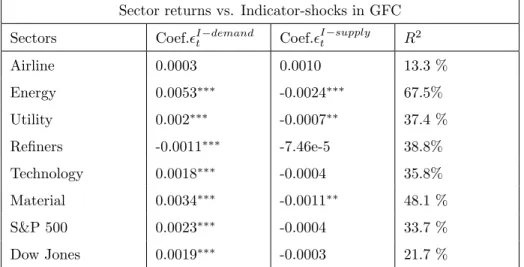
To see whether our models are robust, we also checked how they perform under special scenarios. We include various episodes such as U.S.-led invasion of Iraq, Global Financial Crisis and COVID-19 pandemics.

Sector returns vs. Indicator-shocks in GFC Sectors Coef.✏I demandt Coef.✏

I supply t R2 Airline 0.0003 0.0010 13.3 % Energy 0.0053⇤⇤⇤ -0.0024⇤⇤⇤ 67.5% Utility 0.002⇤⇤⇤ _-0.0007⇤⇤ _{37.4 %} Refiners -0.0011⇤⇤⇤ _{-7.46e-5 38.8%} Technology 0.0018⇤⇤⇤ _{-0.0004 35.8%} Material 0.0034⇤⇤⇤ _-0.0011⇤⇤ _{48.1 %} S&P 500 0.0023⇤⇤⇤ _{-0.0004 33.7 %} Dow Jones 0.0019⇤⇤⇤ _{-0.0003 21.7 %}

Sector returns vs. Structural shocks in GFC Sectors Coef.✏S demandt Coef.✏

S supply t R2 Airline 0.0159⇤⇤⇤ _0.0050⇤⇤⇤ _{41.6 %} Energy 0.0005 0.0147 87.9 % Utility -0.0012 0.0072⇤⇤⇤ _{61.9 %} Refiners 0.0016 -0.0155⇤⇤⇤ _{61.9 %} Technology 0.0026 0.0096⇤⇤⇤ _{56.2 %} Material 0.0068⇤⇤ _0.0121⇤⇤⇤ _{68.3 %} S&P 500 0.0039 0.0087⇤⇤⇤ 59.6 % Dow Jones 0.0033 0.0049⇤⇤⇤ 49.2%

Table 6: Structural shocks vs. Stock market in GFC

5.5

Macroeconomic indicators

5.5.1 Explanatory Models

Oil price change serves as an important transmitter. For example, when there is a signal of upcoming recession, it first reflects in decreasing demand, namely negative demand shock, and then shows up in the oil price change. It’s obvious that the entangling di↵erent side of shocks will show up in the oil price change, and then transmit to the performance of our economy. Hence, we’re going to examine how these shocks explain or predict the next period macroeconomic indicators.

At time t, let Ytdenote the macroeconomic indicator value, ✏I demandt , ✏

I supply t

as the demand and supply shock identified by our new indicator, ✏S demandt ,

✏S supplyt as the demand and supply shock decomposed by the structural VAR

model, and ✏S riskt as the systematic risk shock. Here we examine two kinds of

models.

Yt= ↵ + 1✏S demandt + 2✏S supplyt + 3✏S riskt + ✏t (16)

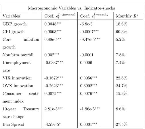
Macroeconomic Variables vs. Indicator-shocks Variables Coef. ✏I demandt Coef. ✏

I supply t Monthly R2 GDP growth 0.0048⇤⇤⇤ _{-6.8e-5 18.6%} CPI growth 0.0003⇤⇤⇤ _-0.0007⇤⇤⇤ _60.3% Core inflation growth 6.88e-5⇤⇤ _-9.47e-5⇤⇤⇤ _5.2% Nonfarm payroll 0.002⇤⇤⇤ _{-0.0001 7.8%} Unemployment rate -0.0337⇤⇤⇤ _{0.0006 7.4%} VIX innovation -0.1672⇤⇤⇤ 0.0956⇤⇤⇤ 22.6% OVX innovation -0.2623⇤⇤⇤ 0.3902⇤⇤⇤ 24.7% Consumer senti-ment index 0.0075⇤⇤⇤ 0.0076⇤⇤⇤ 15.3% 10-year Treasury rate change 2.81e-5⇤⇤⇤ _-1.96e-5⇤⇤⇤ _8.6%

Baa Spread -4.29e-5⇤ _0.0001⇤⇤⇤ _27.5%

Macroeconomic Variables vs. Structural-shocks Variables Coef.✏S demandt Coef.✏

S supply

t R2

GDP growth 0.0003 0.0008⇤⇤⇤ _20.6%

CPI growth 7.25e-6 0.0002⇤⇤⇤ _30.1%

Core inflation growth 7.21e-5 4.99e-5⇤⇤⇤ _5.2% Nonfarm payroll 0.0002 0.0007⇤⇤⇤ _6.8% Unemployment rate -0.0027 -0.0106⇤⇤⇤ _5.2% VIX innovation 0.0064 -1.2310⇤⇤⇤ 36.9% OVX innovation -0.5743⇤⇤⇤ -1.0615⇤⇤⇤ 6.9% Consumer senti-ment index 0.0009 0.0030⇤⇤⇤ 5.4% 10-year Treasury rate change 5.88e-5 0.0002⇤⇤⇤ _13.6%

Baa Spread -4.67e-5 -8.12e-5⇤⇤⇤ _5.9%

Table 8: Structural-shocks vs. Macroeconomic variables

Table 7 presents the empirical results from our crack-spread indicator la-belled shock, and Table 8 shows the results from our structural shocks. Com-bining the previous two tables (Table 5 and Table 6), we can verify that our first method, crack-spread indicator, outperforms the structural VAR model when they explain the macroeconomic shocks. However, when they’re explaining the fluctuations in the stock market, the structural VAR model takes an advantage by including one of the stock return series in the decomposition system, making it contain more information about stock market.

5.5.2 Robustness Testing

Similarly, here we examine how stable these extracted shocks behave under special scenarios.

Macroeconomic variables vs. Indicator-shocks in GFC Variables Coef. ✏I demandt Coef. ✏I supplyt R2

GDP growth 0.0010⇤⇤⇤ -0.0002⇤⇤⇤ 73.8% CPI growth 0.0003⇤⇤⇤ -0.0002⇤⇤⇤ 81.9% Core inflation growth 2.61e-6 -3.52e-5⇤ 31.1% Nonfarm payroll 3.25e-5 -7.47e-5 23.4% Unemployment rate -0.0005 0.0003 9.5% VIX innovation -0.3571 0.2298 48.3% OVX innovation -0.0037 0.7525 34.8% Consumer sentiment

in-dex

-0.0046⇤⇤⇤ _-0.0051⇤⇤⇤ _15.5%

10-year Treasury rate change

3.70e-5⇤⇤⇤ _-3.23e-5⇤⇤⇤ _11.5%

Baa Spread -0.0002⇤⇤ 6.98e-5 49.2% Table 9: Indicator-identified shocks in GFC

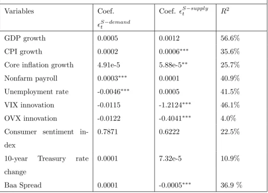
Macroeconomic variables vs. Structural-shocks in GFC Variables Coef. ✏S demandt Coef. ✏S supplyt R2 GDP growth 0.0005 0.0012 56.6% CPI growth 0.0002 0.0006⇤⇤⇤ _35.6%

Core inflation growth 4.91e-5 5.88e-5⇤⇤ _25.7%

Nonfarm payroll 0.0003⇤⇤⇤ _{0.0001 40.9%}

Unemployment rate -0.0046⇤⇤⇤ _{0.0005 41.5%}

VIX innovation -0.0115 -1.2124⇤⇤⇤ 46.1% OVX innovation -0.0122 -0.4041⇤⇤⇤ 4.0% Consumer sentiment

in-dex

0.7871 0.6222 22.5% 10-year Treasury rate

change

0.0001 7.32e-5 10.9% Baa Spread 0.0001 -0.0005⇤⇤⇤ _{36.9 %}

Table 10: Structural-identified shocks in GFC

From Table 9 and 10, we can still generate the idea that the indicator-identified shocks are more stable and robust than structural shocks from the classic model. Generally the R2 _{is higher and coefficients are more significant}

than in the structural model.

6

Conclusion

To conclude, we discover that the shocks identified by the crack-spread indi-cator are more accurate and can explain macroeconomic variables better than shocks identified by structural VAR model. However, if we’re explaining the fluctuations in stock market, the structural VAR model provides more insights and stronger results. Our crack-spread indicator has much promising ability in identifying the main driver of oil shocks.

There are several aspects where we can make improvements in the future. First, our crack-spread indicator enables us to label each period as demand shock or supply shock, but it can only help us recognize the main driver, but not providing us the insight of disentangling the simultaneous shocks on each side. Structural VAR model can achieve this point by constructing this orthog-onal decomposition system. However, it also needs strong assumptions. The decomposition system may not be triangular in the real world. The change of oil production of OPEC is a↵ected by both demand shock and supply shock, instead of being a↵ected by only one side. Second, refined oil has a stable re-lationship with crude oil. The price of refined oil is always based on the raw material costs of crude oil. We can include the mean-reverting patterns to refine the theoretical framework for the crack-spread indicator.

7

References

Kilian, L.(2009). Not all oil shocks are alike. American Economic Review, pp.1053-69

Kilian, L Park, C.(2009). The Impact of Oil Price Shocks on the U.S. Stock Market. International Economic Review, Vol. 50, No. 4, pp.1267-1287

Kogan, L Ahn, D.P.(2012), Crude or Refined: Identifying Oil Price Dynamics Through the Crack Spread. SSRN Electronic Journal, doi:10.2139/ssrn.2024359 Ready, R.C.(2013). Oil Prices and Stock Market. Review of Finance. Vol. 22, No. 1, pp.155-176

Dutta, A.(2017). Oil price uncertainty and clean energy stock returns: New ev-idence from crude oil volatility index. Journal of Cleaner Production, pp.1157-1166

Demirer, R Ferrer, R Shahzad, S.J.H.(2020). Oil price shocks, global financial markets and their connectedness. Energy Economics, forthcoming