HAL Id: hal-01095602
https://hal.archives-ouvertes.fr/hal-01095602
Submitted on 15 Dec 2014
HAL is a multi-disciplinary open access
archive for the deposit and dissemination of
sci-entific research documents, whether they are
pub-lished or not. The documents may come from
teaching and research institutions in France or
abroad, or from public or private research centers.
L’archive ouverte pluridisciplinaire HAL, est
destinée au dépôt et à la diffusion de documents
scientifiques de niveau recherche, publiés ou non,
émanant des établissements d’enseignement et de
recherche français ou étrangers, des laboratoires
publics ou privés.
Inverse rheometry and basal properties inference for
pseudoplastic geophysical flows
Nathan Martin, Jerome Monnier
To cite this version:
Nathan Martin, Jerome Monnier. Inverse rheometry and basal properties inference for
pseudoplas-tic geophysical flows. European Journal of Mechanics - B/Fluids, Elsevier, 2015, 50, pp.110 - 126.
�10.1016/j.euromechflu.2014.11.011�. �hal-01095602�
Inverse rheometry and basal properties inference for pseudoplastic geophysical
flows
N. Martina, J. Monnierb
aCalifornia Institute of Technology’s Jet Propulsion Laboratory, 4800 Oak Grove Drive, Pasadena, CA 91109, United States
bMathematics Institute of Toulouse - National Institute for Applied Sciences, 135 Avenue de Rangueil, 31077, Toulouse Cedex 4, France
Abstract
The present work addresses the question of performing inverse rheometry and basal properties inference for pseu-doplastic gravity-driven free-surface flows at low Reynolds’ number. The modeling of these flows involves several parameters, such as the rheological ones or the state of the basal boundary (modeling an interface between the base and the fluid). The issues of inverse rheometry are addressed in a general laboratory flow context using surface ve-locity data. The inverse characterization of the basal boundary is proposed in a geophysical flow context where the parameters involved in the empirical effective sliding law are particularly difficult to estimate. Using an accurate direct and inverse model based on the adjoint method combined with an original efficient solver, sensitivity analyses and parameter identification are performed for a wide range of flow regimes, defined by the degree of slip and the non-linearity of the viscous sliding law considered at the bottom.
The first result is the numerical assessment of the passive aspect of the viscosity singularity inherent to a power-law pseudoplastic (shear-thinning) description in terms of surface velocities. From this result, identification of the two parameters of the constitutive law, namely the power-law exponent and the consistency, are performed. These numerical experiments provide, on the one hand, a very robust identification of the power-law exponent, even for very noisy surface velocity observations and on the other hand, a strong equifinality problem on the identification of the consistency. This parameter has a minor influence on the flow, in terms of surface velocities. Typically for temperature-dependent geophysical fluids, a law describing a priori its spatial variability is then sufficient (e.g. based on a temperature vertical profile).
This study then focuses on the basal properties interacting with the fluid rheology. An accurate joint identification of the scalar valued triple (n, m; β) (respectively the rheological exponent, the non linear friction exponent and the friction coefficient) is achieved for any degree of slip, allowing to completely infer the flow regime. Next, in a geophysical flow context, identifications of a spatially varying friction coefficient are performed for various perturbed bedrock topography. The (2D-vertical) results demonstrates a severely ill-posed problem that allows to compute a given set of surface velocity data with different topography/friction pairs.
1. Introduction
Power-law fluids represent a wide category of mate-rials in the range of shear rates to which the coefficients were fitted. Pseudoplastic fluids designate fluids pre-senting a shear-thinning behavior, modeled by a power-law constitutive power-law (e.g. polymer solutions, ice, blood etc) which expresses the relationship between the devi-atoric stress tensor S and the strain-rate tensor D as (see also Section 2.1):
S= 2η0kDk
1−n n
F D (1)
The power-law type description leads to focus on the
two undetermined parameters of such a law which are the exponent of the law n (scalar value) and the rate factor or consistency η0 (possibly spatially distributed)
which are generally hard to estimate in a real context and difficult to measure experimentally (see e.g. [1]). In a geophysical context, these fluids involve gravity-driven mass movements and are generally treated as flu-ids flowing down a slope (see e.g. [2]). They show a complex and non uniform rheology and have a strong dependency on their basal properties, possibly in rela-tion with their rheology. The basal properties mainly involve the modeling of a basal slip through a (possibly non-linear) viscous empirical effective sliding law. The
sliding law is itself a model. It expresses the relation-ship between the basal shear σntand the basal velocity
u · t as (see also Section 2.1):
|σnt|m−1σnt= βu · t (2)
It includes a friction parameter β which is hard to directly estimate and an exponent m describing the nonlinear response of the subglacial material on which the sliding occurs. It is in this context that the possi-bility of inferring these quantities (and consequently the model they describe) through inverse modeling becomes essential.
In the case of scalar valued parameters, the identi-fication of rheological components formulated as an inverse problem (thus using a direct differentiation of the problem) has been treated in an industrial context (particularly metal forming), adapted to particular experimental setups only. Following this type of ap-proach, identification of rheological parameters based on cross-section velocity measurements can be found in [3, 4]. A similar approach using measurement of a pressure drop is proposed by [5]. In [6], attention is also payed to the identification of a scalar friction parameter.
The present study aims to perform inverse rheometry in a more general context, hence applicable to broader
experimental setups. In addition, the present study
focus on geophysical flows whose characteristics
are: uniqueness of a given situation (compared to
reproducible laboratory experiments), velocity obser-vation generally limited to the surface and a possible strong influence of an unknown and unmeasurable basal slip modeling an heterogeneous basal interface non linearly interacting with the bed and the flow. We focus hereafter on a pseudoplastic representative geophysical examples which is ice flows. In ice flows modeling, the power-law model firstly presented in [7] is well admitted; while its temperature and shear rate dependency is still a matter of debate (see e.g. [8], [9]). The coupling with thermal physics also occurs in the definition of the consistency.
For instance, the present equations are also suited for
modeling lava flows. In this case, the question of
the power-law index value is still under debate and has been widely discussed but the literature generally agrees on a pseudoplastic (shear-thinning) behavior of the magma with possible dependency of this exponent on temperature and/or crystal concentration (see e.g. [10]).
The present studies are mainly led in this geophysical fluid flow context, but the method and the results, when mentioned, can be extended to general experimentally controlled flows in laboratory experiments. Also, the model and methods developed here are also valid for dilatant (shear-thickening) fluids but has not been numerically explored.
If the fluid flow present basal slip, the latter becomes a major component of its modeling. Thus, investiga-tions regarding the physical components and relevant parameterizations introduced in the (empirical effective) friction law are of primal importance.
In the case of ice and lava, different laws are used to evaluate this parameter but a common description is to consider an Arrhenius-type law including ap-propriate physical considerations, see e.g. [8] for ice and [11] for magma. In glaciology, the basal friction law models the subglacial water pressure, underlying non linear till, surface roughness, geothermal heat flux etc, see eg [8]. The identification of the basal friction coefficient and the consistency in glaciers models using a variational approach became quite common recently but considering the ice viscosity to be independent of the velocity in the "adjoint model" derivation, hence simplifying greatly the inverse model but leading to the computation of an incorrect gradient. The continuous adjoint model in the glaciological context, with nonlinear basal slip, can be found in [12]. In other respect, the question of basal properties characterization through surface velocity observations using the present variational approach is studied in [13]. In a computational point of view, the present study is based on a second-order forward and adjoint solution for the power-law Stokes problem. The forward prob-lem, written as a four-field saddle point formulation of the power-law Stokes problem, is discretized with three-field finite elements and solved using a splitting technique and an augmented Lagrangian approach (providing large cpu-time saving, see [14]). The adjoint problem is solved using source-to-source automatic differentiation of the augmented Lagrangian algorithm. The newly obtained adjoint solver provides a second order accuracy gradient, efficiently computed and with low memory needs. Ratios of four (4) in cpu-time and memory consumption are assessed, compared to the differentiation of a classical fixed-point based solver. We refer to [13] for the technical method to assess the gradient accuracy.
In any case, what can be obtained from an inverse approach is strongly related with the type and quality of available data. This study focuses on the use of surface horizontal velocity data (generally the most dense and accurate data in the present geophysical context, see e.g. [15]) to constrain the rheology and the basal properties of this type of flow depending on the flow regime. All the numerical experiments are designed according to the bounds in terms of basal variability
transmission to the surface assessed in [13]. The
experiments are carried out on steady state geometries of the free-surface gravity-driven flows.
As a preliminary issue, this study numerically address the role of the well-known viscosity singularity at the surface (i.e. at vanishing shear-rate) in the power-law shear-thinning constitutive law, in an inverse context, relying on surface velocity observations. As a matter of fact, this singularity might lead to an ill-posed direct problem if a free-surface is considered as pointed out in [16]. For different sliding regimes, sensitivity analysis demonstrate that the refinement of the mesh close to the surface, while leading to the appearance of a stiff (very high viscosity) layer, does not affect the solution and that the viscosity singularity remains passive in the model confirming numerically the analysis done in [17].
From this result, numerical experiments of virtual
rheometry are carried out. Identifications of the
scalar power-law exponent first, and then sensitivity analysis and identification of the spatially distributed consistency are performed. The identification of the power-law exponent proves to be extremely robust (providing a highly accurate identification for a 50% noise on the data), regardless of the flow regime. Con-versely, the identification of a temperature-dependent consistency is a severely ill-posed problem, even with very good prior physical intuitions introduced in the initial guess and the regularization term, leading to a strong equifinality issue. We conclude that the consistency has a negligible role in the model in the bulk and that a trustworthy modeling a priori of the temperature-dependency is sufficient.
Based on this result, we then perform identifications of the scalar-valued triple (n, m; β) (respectively the power-law exponent, the friction law exponent and the friction coefficient) for all situations of sliding (from strong friction to high sliding). The results are fully conclusive allowing to accurately infer these three scalar quantities and therefore the regime of the flow,
based only on surface velocity observations.
The final step is to identify (typically using the scalar identification as a very good initial guess) a spatially varying friction coefficient β. The numerical experiment is designed in order to explore the typical regimes of sliding of an ice-stream flow (from medium friction to very rapid sliding), with relevent length scales for the basal variability chosen following [13]. Based on a ref-erence simulation, representing a “true state”, simula-tions on randomly perturbed bedrock topographies are performed. The main result is the fact that the inferred friction coefficient completely depends on the topogra-phy in order to produce a given set of surface velocity data. This final result point a strong equifinality prob-lem for the topography/friction pair and raises a ques-tion on how it affects the predictive capabilities of ice flow models since the most poorly observed data is the bedrock topography.
2. Forward Model
In this section we present the key aspects of the fluid model considered in the present study and its numerical approximation.
2.1. Continuous Model
The flow is assumed to be 2D vertical (in (x, z) co-ordinates); it is modelled as an incompressible viscous
fluid in a time moving domain Ωt open, bounded and
connected in R2 with boundary ∂Ω (assumed to be
Lipschitz). The momentum balance is described us-ing the incompressible Navier-Stokes equation with low Reynolds approximation, thus by the so-called Stokes equation. The flow is driven by the gravity source term. The forward model equations are:
−div(σ)= ρg in Ωt (3)
div(u)= 0 in Ωt (4)
where u = (ux(x, z, t), uz(x, z, t)) ∀(x, z) ∈ Ωt, t ∈
[0, T ] denotes the velocity, σ the Cauchy stress tensor, ρ the fluid density, g the gravity and Ωtis the domain at
time t. The stress tensor σ is decomposed as:
σ = −pId + S (5)
where S is the deviatoric (or extra) stress tensor, p the pressure and Id the unit tensor. The non Newtonian vis-cous behavior is described by a viscoplastic constitutive law that relates the stress tensor to the strain-rate tensor. A power-law model, first proposed by Ostwald in 1925
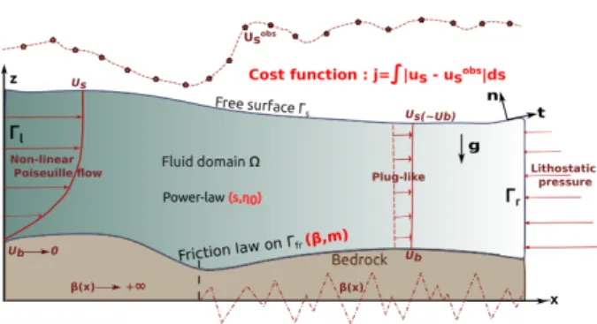
Figure 1: Typical geometry of the free-surface geophysical flow
con-sidered. Notations of the geometry and the boundary conditions.
Schematic representation of the inverse problem where usand ub
des-ignates surface velocity and basal velocity respectively and uobs
s
des-ignates isolated surface velocity measurements. The control variables are represented in bold red as well as the typical cost function and are
β, m, n and η0(see end of Section 3.2).
(see e.g. [18]), is considered hereafter. It follows that the deviatoric tensor S is written as:
S= 2η(u)D with η(u) = η0kDk
1−n n
F (6)
where η is the apparent viscosity, D=12(∇u+ ∇uT) the strain-rate tensor, n the power-law index and the consis-tency η0(also called rate or creep factor in glaciology)
is a dimensional constant which can depend on the state of the considered fluid (typically the temperature). The Frobenius matrix norm k · kF usually called the
shear-rateis defined by:
kDkF=
r 1 2tr( D D
T)= ˙γ (7)
A typical domain is represented in Figure 1. The
surface Γs, considered to be the graph of a function
h(x, t), is a free surface moving in time. The boundary ∂Ω is divided as follows: Γsis the moving surface (free
surface),Γbis the bottom surface,ΓlandΓrare lateral
open boundaries.
The free surface dynamic is described by the follow-ing 1D transport equation:
∂th+ ux∂xh= a + uz onΓs× [0, T ] (8)
with a modelling a mass balance source term. Boundary conditions.
We introduce (t, n), the normal-tangent pair of unit vectors such that:
σ = (σ · n)n + (σ · t)t (9)
with:
σ · n = σnnn+ σntt , σ · t = σtnn+ σttt (10)
On the top surface Γs we consider a traction-free
boundary condition while given stress or Dirichlet con-ditions can be prescribed on the lateral boundaries Γl
and Γr. The boundary Γb is splitted into an
homoge-neous Dirichlet areaΓadand a friction (or sliding) area
Γf r. The friction/sliding law on Γf ris a power-law type
law (also known as Weertman law, see e.g. [8]) given by:
|σnt|m−1σnt= βu · t on Γf r, u · n= 0 on Γf r (11)
where m is the stress exponent and β is the friction coefficient. This viscous friction (or sliding) law is an entire model itself as it can represent bedrock heterogeneities, material properties change, an unclear
interface, etc. Typically, in glaciology it aims to
model the non-linear rheology of a subglacial sediment layer (through a parameter m > 1) and the water pressure from underlying hydrology (typically setting
β = kNq, q ≥ 1 and N = ρgh − P
water the effective
pressure).
Also, there is no consensus on the value of m (or q) a classical choice for ice-streams flows consists to set m= 3, (and q = 1, see e.g. [8]). In a nutshell, the fric-tion coefficient β is a priori non uniform and depends on various quantities (bedrock roughness, subglacial water pressure, sediment properties, etc) and requires to be ac-curately calibrated. The last section of the present paper focuses on this question.
The boundary conditions on the lateral boundaries
are as follows. At inflow, we impose the vertical
velocity profile as the shallow power-law uniform solution, see e.g. [19]; a lithostatic pressure is imposed
at the outflow boundary. The boundary conditions
on the lateral boundaries are as follow;. at inflow, we impose the vertical velocity profile as the shallow
power-law uniform solution, see e.g. [20, 19]; at
outflow, a lithostatic pressure is imposed.
2.2. Numerical solution of the forward problem The numerical solution of the forward model (3)-(4) is obtained using the four field finite element scheme, of order two in space, and the augmented Lagrangian type algorithm detailed in [14]. Such a formulation arises when applying a splitting technique on a minimal dis-sipation form of the corresponding variational problem.
The splitting, by introducing the strain-rate tensor D as an unknown, allows the linear part and the non linear part of the governing equations to be solved sequen-tially. This algorithm provides important cpu-time sav-ing compared to a classical fixed point approach as well as memory saving (which becomes important for solv-ing the adjoint problem, as in Section 3). This formula-tion requires a three-field finite element discretizaformula-tion in order to handle the tensorial unknowns D and S in addi-tion to the vectorial unknown u and the scalar unknown p (see [21]). We refer to [14] and references therein for a complete assessement of this accurate and robust second order finite element scheme.
Free surface dynamic. Recall thatΓsis supposed to be
the graph of a function h(x, t), an Arbitrary Lagrangian Eulerian (ALE) formulation is adopted for the treatment of its dynamic. The mesh velocity is computed from the solution of an elastic problem or from a vertical homo-thety if appropriate. Equation (8) is solved using the characteristics method; it gives:
∂th+ ux∂xh= dh dt χ= a + uz , RHS given (12)
where χ denotes the characteristic curves. Then for each node, we obtain a Cauchy problem which can be solved using classical schemes (here Euler or Runge-Kutta or-der 2). In the present study, inverse rheological ques-tions are investigated and the numerical experiments are only performed on steady state situations. The steady-state steady-state is obtained by running in time the free-surface model until the average relative normal velocity (dis-crete 1-norm) at the vertices is lower than 10−4and the
relative variation of volume is lower than 10−5.
Figure 2: Four-field FEM implemented: extended Taylor-Hood mixed
finite elements corresponding to a P2continuous velocity, P1
contin-uous pressure and P1 discontinuous strain rate and deviatoric stress
tensors.
3. Inverse model
This section briefly describes the adjoint-based method used in the present work to investigate inverse
questions (sensitivities, data assimilation -
identi-fication). The resulting numerical tool is accurate
since gradients are of second order. Furthermore it is efficiently computed since based on the newly obtained differentiation of the four-field finite element solver presented previously.
3.1. Cost function and optimization problem
The output of the model is represented by the cost function j (a scalar valued function) which depends on the parameters k of the model. Given velocity observa-tions denoted uobs, we define the cost function j which
measures the discrepancy between the computed vari-able (state of the system) and the availvari-able data at a given time. Extra terms can be added to the definition of the cost function to include n a priori on the physics of the control variables and/or a regularization of the opti-mization problem:
j(k)= Z
kCuobs− u(k)k22dx+ regularization terms (13) where u is the computed velocity of the system and Cis the observation operator.
The optimization problem writes: min
k j(k) (14)
This minimization problem is solved numerically by the quasi-Newton local descent algorithm L-BFGS im-plemented in the M1QN3 routine (see [22]). To do so, the gradient of j has to be computed. The corresponding procedure is described hereafter.
3.2. Adjoint model and gradient accuracy
The cost function gradient is deduced from the
adjoint code of the forward direct code. The direct
code, solving the power-law Stokes problem at order two in space, is written in Fortran 95. The development of the sensitivity and parameter identification modules are part of the DassFlow project which was originally designed for shallow-water models, see [23, 24, 25]. The present code, called DassFlow-Ice (or DassIce), has been developed during the PhD of the first author (see [26]) and is publicly available (see [27]).
There exists three approaches in order to obtain a solution algorithm of the adjoint problem. The most natural one called continuous appproach consists in analytically derive the continuous adjoint model and
then discretized it with any appropriate numerical scheme. The main difficulty of this approach lies in the potentially difficult analytical derivation, sometimes requiring some simplifying assumptions to be achieved. Conversely, the discrete approach consists in deriving the adjoint model of the discrete formulation of the forward model. This method ensure a good consistency between the forward and the adjoint discrete models.
In DassFlow software, the adjoint model is obtained by using algorithmic differentiation of the source code (which is a particular case of the discrete approach). The principle of algorithmic differentiation is based on the idea that any numerical program is a sequence of elementary operations that can be analytically derived with the usual derivation rules.
Let us consider the forward code as an operator M : Rn → Rs that computes for a set of input parameters k ∈ Rn, an output vector Y ∈ Rs. One denotes by m
k
an elementary operation and by Xk−1 the value of the
variables at step k. If one includes the control vector k in the global set of variables for the program (k ⊂ X0) ,
one can write:
Y = M(k) = mp(Xp−1) ◦ mp−1(Xp−2) ◦ ... ◦ m1(X0) (15)
The Jacobian matrix of M is then given by: ∂M
∂k (k)= m0p(X p − 1) × m 0
p−1(Xp−2) × ... × m01(X0) (16)
where m0kare the Jacobian matrices associated to the elementary operations mk.
Tangent mode. In practice the Jacobian matrix (16) is too complicated to be computed and to heavy to be stored in memory. However one can compute a direc-tional derivative associated to a given direction δk:
∂M
∂k (k) · δk= m0p(X p − 1)×m 0
p−1(Xp−2)×...×m01(X0) · δk
(17) where the computation is performed from the right to the left by simple matrix-vector products. This method leads to obtain the linear tangent model by algorithmic differentiation.
Reverse mode. The remaining issue is that the linear tangent model is not appropriate to compute the gradient since it requires s integrations (for a solution vector in Rs). Automatic differentiation in reverse mode allows to compute the scalar product between the transposed
of the Jacobian matrix (i.e. the adjoint model) and a vector eY: ∂M ∂k (k) ! · eY = m0T1 (X0) × m0T2 (X1) × ... × m0Tp (Xp−1) · eY (18) This expression is also computed from the right to the left by a sequence of matrix-vector product.
The automatic differentiation approach ensures a
better consistency between the computed cost function and its gradient and a high accuracy of the computed gradient, since it is the computed cost function that is differentiated. A large part of this extensive task can be automated using automatic differentiation (see [28]).
The linear solver used is MUMPS ([29]) and the differentiation of the linear system solving process is achieved using a “bypass” approach which considers the linear solver as an unknown black-box (see [13]).
The adjoint code is derived using the automatic differentiation tool Tapenade (see [30]).
Let us notice that the continuous exact adjoint system of the power-law Stokes equations is presented in [31] for a general optimal control framework and in [13] for the problem with a nonlinear friction boundary condition (treated in the present work).
A single integration of the forward model (3)-(4) followed by a single integration of the adjoint model allow to compute all components of the gradient of
the cost function. The computed gradient has been
validated against order two finite differences and is adjustable in precision (from the fully incomplete gradient corresponding to the so called “self-adjoint” method in the glaciology community, to the exact order two accurate gradient) providing time and memory saving for an identical precision (see [13, 14]).
We consider in the following, as control variables, the two parameters of the rheological law which are the consistency η0 and the power-law exponent n (see (6))
and the two parameters of the friction law which are the friction coefficient β and the exponent m (see (11)). Therefore, we set k= (n, η0) and we write the total
dif-ferential d j of the cost function j as follows: d j(k) = ∂η∂ j
0(k) · δη0+
∂ j
∂n(k) · δn+∂β∂ j(k) · δβ+∂m∂ j(k) · δm
(19) The output of the adjoint code corresponds to the partial derivatives of the cost function j with respect to the
chosen control variables.
Every variable in the control vector is only a potential control variable. In practice, it is possible to identify only a few of them simultaneously.
3.3. Local Sensitivity Analysis
Let us consider s parameters to be controlled i.e. k is a vector value of size s. Then, the s gradient value components, j0(k) = (∂k∂ j
i)1≤i≤s, give the sensitivity of
the output function j with respect to the ithcontrol com-ponent, at the point k.
The sensitivity analysis allows to study how perturba-tions on the input parameters of a model lead to a per-turbed output. The use of an adjoint model provides a local sensitivity analysis around a given point by com-puting the Fréchet derivative of the cost function j (e.g. defined by (13)) with respect to the control variables k. This sensitivity analysis tool is an important fea-ture which provides a better understanding of both the physics and the model by quantifying the roles of the various physical parameters and the influences of pa-rameter variations on the behavior of the system. Since control parameters can be spatially distributed, the re-sults can be sensitivity maps (e.g. sensitivity maps with respect to the consistency η0).
3.4. Data Assimilation and Twin Experiments
The main goal of the present article is to investigate the sensitivities and inference capabilities of a varia-tional method for geophysical free-surface flows with a power-law rheology, with respect to the rheological
parameters and the basal properties. To do so, we
design in next sections fully representative flows in term of regimes, and twin experiments including realistic noised surface observations are performed.
Twin experiments are defined as follows. The refer-ence parameters of the model kre f are used to generate
observations uobs. Then, the goal is to retrieve the set of
parameters kre f starting from an initial guess k , kre f
using the minimization of the cost function j. In order to avoid the so called inverse crime and to simulate re-alistic situations, a random Gaussian noise is added to the synthetic data obtained from the numerical model. 3.5. On the efficiency of the adjoint solution based on
the four-field finite element solver LA
Since the adjoint code is obtained from
source-to-source automatic differentiation of the forward
code, the performances of the adjoint computation are strongly linked to the algorithm considered for the solution of the forward problem. In the present case, automatic differentiation has been applied to the imple-mentation of the augmented Lagrangian type algorithm called LA. It is described and assessed in details in [14].
The automatic differentiation of an iterative proce-dure is handled using a reverse accumulation technique. It consists in computing a partial derivative associated to each state encountered by the forward solver. The final adjoint state is then computed as the sum of the partial derivatives (as a consequence of the chain rule). This process a priori requires to store as many states of the system as iterations performed by the forward solver to reach the converged state. We address [13] for a comprehensive description of this approach.
This procedure applied to LA algorithm allows very good performances to be obtained compared to the derivation of a fixed point type algorithm. Firstly, an important time-saving is obtained according to the time-saving provided by LA algorithm for the solving of the forward problem. Secondly, the splitting consid-ered in LA algorithm implies that the Stokes system is not modified along the iterations. It therefore requires
only one factorized Stokes stiffness matrix to be
stored. The non-linear tensor equation, discretized on a discontinuous finite element basis, is block-diagonal and therefore solved along the assembly. It follows that no storage of this matrix is required.
The present implementation allows to obtain for the complete solution (i.e. the forward solution plus the adjoint solution), compared to the fixed point approach used in [13], on a mesh of 300 000 elements, a cpu-time ratio of 5 and a memory ratio of 4 . These ratios are smaller than one can expect, based on the ratio obtained for a single forward solve, due to a non-robust behavior of the Newton algorithm used to solve a non-linear scalar equation on the norm of the strain-rate within
the algorithm (see [14]). The use of a more robust
algorithm could allow to significantly improve these ratios.
In other respect, technical adjustements in terms of checkpointing can provide, using more memory, a better cpu ratio.
4. Assessment of the inverse numerical model: sur-face observations and near-sursur-face singularity 4.1. Issue addressed
The power-law form is an empirical fit to laboratory and field data within a finite shear rate range. But, this law leads to an infinite viscosity singularity for van-ishing shear-rates (in the shear-thinning case, n > 1, see equation (6)). In other respect, it has been demon-strated that this singularity might lead to an ill-posed direct problem if a free-surface is considered (see [16]). In a geophysical fluid flows context, measurements of rheological parameters are difficult and may depend on the experimental setup, the shear-rate range and, for fluid such as ice or lava, on the temperature (see [8], [11], [32]). For instance, the laboratory conditions will generally differ from the field. It follows that the values for both the power-law exponent n and the consistency η0are not clearly established.
In the glaciology context, and concerning the infinite viscosity singularity at the free-surface, in [33] for example, the author proposes a regularization at low
shear-rate by adding a constant (i.e. a Newtonian
threshold). In [17] the authors consider the Glen’s
power-law (without low shear rate regularization and using n= 3), a locally perturbated topography (around a mean slope) and a friction condition at the bottom. Using shallow asymptotic expansions (i.e. with respect to the aspect ratio ε) and matching techniques between the near-surface layer and the "bulk" solution (far from the free surface), the authors give explicit expressions of the stress components and velocity fields at the free surface. At the leading order (first order in ε), the stress components σxx, σxz are unphysically singular. They
show that the singularity appears in a boundary layer of size O(ε1/3), which might not be negligible in practice.
The authors show nonetheless that at first order in ε, the singular solution remains "passive", in the sense that the free-surface geometry may not be changed because of the presence of the boundary layer. In other words, for shear-thinning shallow flows, one should be able to infer basal behavior from surface velocities, using a power-law model without any (non physical) regularization at low shear rate.
Since surface velocities may be used to invert the fluid properties studied, since all inversions on the considered geophysical flows are based on surface ob-servations, it seems to be relevant to assess the present inverse approach inferring capabilities "through" this
singular boundary layer. It is what we propose to
numerically assess in the experiments below.
4.2. Methodology of investigation
In order to address this question, given horizontal surface velocity observations, we compute sensitivities with respect to a locally defined power-law exponent n. It means that the solving of the adjoint code provides a gradient of the cost function with respect to n around a constant value n= 3.
Test case design. We consider the flow occuring in a non uniform slab with a perturbated sinusoidal bottom. The shape of the bottom is built as a carrier sinusoidal function b0 perturbed with two higher frequencies b1
and b2. The carrier wave has an amplitude a0 = 2/5¯h
with ¯h = 1000m the average thickness and the two
perturbations have an amplitude a1 = a2 = 1/5¯h. The
frequency of the carrier wave is f0 = 5¯h and the two
perturbations have frequencies f1 = 2¯h and f2 = ¯h.
This topography has been built according to the results given in [13] providing the fact that, using dense surface velocity observations with a 1% noise, the basal variability frequency transmits to the surface up to two thicknesses; higher frequencies does not a priori affect
the surface. The computational domain presents an
aspect ratio of 1/10 on a 2% slope. The inflow on the left boundary is given by the analytical Poiseuille type solution of the power-law uniform stationnary flow (see e.g. [13]). The boundary condition at outflow is a prescribed lithostatic (ice) pressure. The simulation is run in time until a steady state is reached. The resulting stationnary free-surface flow is thus obtained.
Considered flow regimes. Two different regimes are
considered in the following sensitivity experiments cor-responding to a low sliding and a rapid sliding at the bottom. The level of sliding is defined using the slip ratio r which quantifies the relative contributions of the viscous deformation and the sliding on the surface ve-locities. It is defined by:
r= u¯b ¯ us− ¯ub
(20) where ¯ub and ¯us represent respectively the average
velocity at the bottom and the surface. In what follows, the low sliding case corresponds to an average slip ratio rl = 0.05 which leads to surface velocities of
sheet regime; 95% the surface velocity comes from the viscous deformation of the ice. The rapid sliding
case corresponds to an average slip ratio rr = 20
which leads to surface velocities of 50m/y to 500m/y typical of an ice stream regime; 95% of the surface velocity comes from the basal sliding. A linear sliding
law, corresponding to m = 1, m defined by (11), is
considered. Surface velocity data uobs
s are generated
for these two situations and a cost function is defined as:
j(n)= Z
Γs
kus(n) − uobss k22dx (21)
The approximation of a near-surface singularity is assessed using two different meshes; an isotropic one and mesh refined at the surface. The surface refinement allows to converge to the singularity as the size of the element goes to zero. Hereafter, a “boundary layer” of 1/5 of the average thickness ¯h is discretized with an element size ratio of 10 compared to the elements in the bulk.
4.3. Numerical results
Figures 3 and 5 plot the resulting sensitivity of the model with respect to the power-law index n defined by element ∂ j/∂n(uobs, n0) using the cost function (21)
for both meshes and the two different flow regimes
(r= 0.05 and r = 20 respectively). The corresponding shear-rates ˙γ (see equation (7)) are plotted in Figures 4 and 6 for both slip ratios. It highlights the strong yet varying correlation between ˙γ and the computed gradient.
In all the following plots, the bounds of the colorbars have been modified to match one another in order for the figures to be compared. The values displayed under the color bars as min and max give the original
bounds of the plotted field. Plots have been cut on
the sides to remove the sensitivity values close to the lateral boundaries, particularly the Dirichlet boundary Γl, which are not representative of the variations sought
since the lateral boundary conditions are fixed.
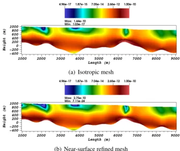
Analysis of the low sliding case (r = 0.05). The case of strong friction at the bottom shows a relatively layered repartition of the sensitivity ∂ j/∂n from high at the bottom to low at the surface for both meshes
(see Figures 3(a) and 3(b)). These sensitivity maps
are strongly related to the shear-rate fields which are naturally decreasing from the bottom to the surface
(a) Isotropic mesh
(b) Near-surface refined mesh
Figure 3: Slip-ratio r = 0.05: Local sensitivity ∂ j/∂n computed
around a state n0= 2.25 using observations uobsobtained with n= 3.
The color scale is logarithmic. The gradient values, constant by ele-ment, have been normalized by the area of their element in order to remove the weight the element size induces (which is a normal feature in an optimization perspective but prevents from drawing a readable sensitivity map on an anisotropic mesh).
(a) Isotropic mesh
(b) Near-surface refined mesh
Figure 4: Slip ratio r= 0.05: Computed shear-rate ˙γ for the observed
state (with n= 3) in s−1. The color scale is logarithmic.
(due to the strong friction condition which induces a non-linear Poiseuille flow, see Figures 4(a) and 4(b)). The mesh refinement at the surface approximates the infinite viscosity but the discretization induces a cut-off on the shear-rate that depends on the size of the elements. The convergence to the viscosity singularity is clear since the minimum shear-rate obtained on the
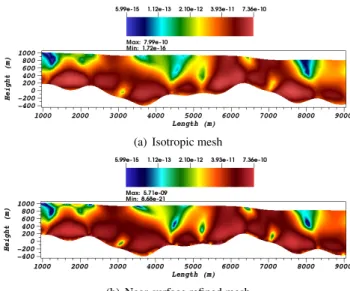
(a) Isotropic mesh
(b) Near-surface refined mesh
Figure 5: Slip-ratio r= 20: Local sensitivity ∂ j/∂n computed around
a state n0 = 2.25 using observations uobsobtained with n= 3. The
color scale is logarithmic. The gradient values, constant by element, have been normalized by the area of their element in order to remove the weight the element size induces (which is a normal feature in an optimization perspective but prevents from drawing a readable sensi-tivity map on an anisotropic mesh.
(a) Isotropic mesh
(b) Near-surface refined mesh
Figure 6: Slip ratio r= 20: Computed shear-rate ˙γ for the observed
state (with n= 3) in s−1. The color scale is logarithmic.
refined mesh is much smaller than the one obtained on the isotropic mesh. However, both the gradient and the shear-rate distribution look identical for both meshes. It follows that a good convergence of the solution was achieved on the coarser mesh and that the refinement of the singularity does not affect the solution. In particular, the singularity remained passive in terms of normal
surface velocities in the transient simulation since the steady state free surfaces are identical for both meshes.
Analysis of the rapid sliding case (r = 20). In the
case of rapid sliding (Figure 5 and 6), the correlation between the shear-rate and the sensitivity is less clear. The presence of a rapid sliding allows high shear rates to develop close to the surface and the layered repartition of the shear-rate (from high shear-rate at the bottom to low shear-rate at the surface) observed for low sliding is no longer observable. Alongside this aspect, the sensitivities ∂ j/∂n show non trivial low sensitivity zone in highly sheared area.
However, as well as the case of low sliding, both meshes show an identical result for the sensitivities ∂ j/∂n. The refined boundary layer does not affect the sensitivity map leading to the same conclusions on the role of the singularity. We point out that the higher absolute values for the gradients in the case of rapid sliding, compared to the low sliding case, are only due to higher surface velocities and therefore a higher misfit. The observed independance of the solution and the gradient with respect to the power-law exponent to the surface velocities numerically assess the robustness of such data to the viscosity singularity.
Based on these results, the next sections focus on the inference of the rheology and basal properties of this type of flow based on surface velocity observations.
5. Virtual Rheometry: constant power-law expo-nent identification
The present identification is performed on a radar-sensed topography of an ice flow with a complex bottom shape but the results can be extended to general experimentally controlled flows with simpler bottoms.
The computational domain considered is built from the radar-sensed topography and bedrock of the Mertz ice-tongue in East Antarctica measured along a flowline
(American program ICECAP 2010, see [34]). It is
plotted in Figure 7. The present study focuses on the grounded part of the glacier which has an average thickness of 1km. The simulation is identical (in terms of boundary conditions) to the one presented in Section 4.2. the friction coefficient β is adjusted accordingly to the two flow regimes (corresponding to average slip
Figure 7: Vertical cut of the outlet glacier Mertz, Antarctica (topography profile from ICECAP 2010 within Ice bridge, provided by B. Legrésy,
LEGOS, France), x-scale= 2/5. The norm of the velocity is plotted in the low sliding case (r = 0.05). The mesh is made of 4000 triangular cells
on approximatively 10 layers.
ratios r= 0.05 and r = 20).
From the results of the previous section, considering the reliability of surface velocity observations, we propose hereafter to use the data assimilation as a complementary numerical tool to support rheometrical investigations of power-law fluids such as laboratory measurements (see e.g. [32]) or estimation from real context data (see e.g. [35]).
We then present identification results of the scalar valued power-law exponent n using noisy synthetic data. These numerical experiments lead to what can be called a virtual rheometer. The cost function is defined by:
j(n)= Z us(n) − u obs s (nt) 2 2 dx (22)
Since a scalar value is identified, there is no need
for regularization. Likewise, the adjoint model is
unnecessary for identifying a scalar value but is used anyway.
Two data sets with Gaussian noise of 10% and 50%
are considered for the experiments. For both data
sets, the decreasing of cost and gradient as well as the evolution of the power-law index value along the data assimilation process are plotted in Figure 8 for the case r = 0.05 using as a first guess n0 = 1. The case of
rapid sliding (r = 20) provides identical results and is consequently not plotted.
Firstly, the almost linear decreasing of cost and gra-dient (on a logarithmic scale) for each situation demon-strates the robustness of the identification of a scalar value. What is also of importance is the extremely large decreasing of the gradient. As a matter of fact, the
gra-0 10 20 30 40 50 Iterations 10-26 10-24 10-22 10-20 10-18 10-16 10-14 10-12 1010-10 -8 10-6 10-4 1010-2 0
Relative cost and gradient
Cost for 10% noise
Gradient for 10% noise
Cost for 50% noise
Gradient for 50% noise
0 5 10 15 20 25 30 35 40 45 Iterations 1.0 1.5 2.0 2.5 3.0 Rheological exponent n
Identified parameter n for 10% noise
Identified parameter n for 50% noise
Target parameter n
Figure 8: Slip ratio r = 0.05: relative cost and gradient during the
data assimilation cycle for different levels of noise. Identified n along
the data assimilation cycle. Relative errors εn=|n−nntt|(with nt= 3 the
target) are: εn= 0.011% and εn= 0.055% for 10% and 50% of noise
respectively
dient decreases by (more than 20 orders of magnitude). This is due to the fact that the model is highly sensitive to the rheological exponent n.
As can be see in Figure 8, the final calibrated value
n is very close to the target value nt even for 50%
perturbed surface velocities. Once the target value is reached, the gradient norm quickly drops to a very small value making clear that the optimum has been reached. It follows that velocity data with large uncertainties are sufficient to recover the uniform value of n.
rheometric measurements are more difficult to access than velocities, or simply inaccessible, even for poorly observed velocities such as e.g. extraterrestrial rheology estimation, see [36].
6. Virtual rheometry: identification ofη0
(tempera-ture dependency)
As we have seen in the previous section, surface velocities represent a robust information to characterize the rheology of a uniform stationary flow. The present approach for the characterization of the power-law exponent led to a virtual rheometer. The other major component of a power-law description is the consis-tency η0(see equation (6)), which allows to characterize
the non-homogeneity of the fluid. It is related, in the case of ice or lava, to spatially non uniform coupled physical effects such as the composition (ice fabric or lava crystal fraction) or thermal physics, hence difficult to assess.
This section focuses on the sensitivity analysis of the steady-state model with respect to a thermal-dependent consistency η0(T ) in order to observe and assess the role
the temperature plays in the flow in terms of surface velocity through this parameter. This context is taken as an example of fluids where the spatial variability (through the temperature-dependency) is expected to be strongly influent.
Then, following the idea of a virtual rheometer, iden-tifications of this distributed parameter are performed using synthetic data for a noise level of 1%.
6.1. Description of the Thermal Dependent Flow As well as lava, ice is considered as a pseudoplastic (shear-thinning) fluid. It is described by a power-law constitutive law called Glen’s flow law which is gen-erally considered to be temperature-dependent. In the case of a non-isothermal glacier, the temperature field is generally obtained using a coupled thermo-mechanical model for the ice. In the sequel, a steady-state tem-perature profile with a zero accumulation term, which corresponds to a linearly decreasing temperature T with respect to the height ¯z is considered (see e.g. [8]):
T(¯z, λ)= Ts−λ¯z (23)
with Tsthe surface temperature and λ the temperature
gradient. It can take a large range of values. In order
to study the effect of the temperature description of the consistency, a large temperature gradient λ = 0.04K/m corresponding to a difference of 40◦C between the
surface and the bottom for a 1km thick glacier is con-sidered hereafter. The surface temperature is therefore Ts= 233.15◦K.
The consistency η0(T ) is obtained from the thermal
law given in [8] written as follows: η0(T )= ηre
−Q
RT (24)
where ηr is the reference viscosity, R is the gas
constant and Q stands for an activation energy. In
glaciology, the power-law exponent n is generally taken equal to 3 and the values of ηrand Q are given (see [8]
for ice and [11] for lava).
The range of temperature within the fluid can be much higher for lava but the definition and parameteri-zation of the law leads to similar consistency gradients. The numerical experiments aim to compare, for a given situation of sliding, an isothermal flow and
a thermal dependent one. The isothermal runs are
identical to those considered in Section 4.2 and the thermal dependent ones use a consistency η0described
by relation (24). Again, every computational domain correspond to the free-surface flow at steady state. Four situations are therefore obtained corresponding to the
two cases of sliding (r = 0.05 and r = 20) with and
without a thermal description of the consistency. Firstly sensitivity analyses are presented for the isothermal and the thermal dependent case for a given slip ratio. Identifications of the thermal dependent consistency are then performed.
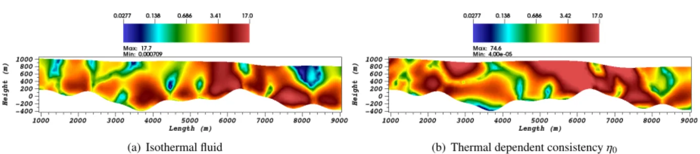
6.2. Sensitivity with respect toη0
Situations of low and rapid sliding at the bedrock
are compared hereafter. It can make an important
difference in terms of sensitivity with respect to η0 by
influencing the flow regime. Figures 9 and 10 plot the
computed shear-rate for low sliding (r = 0.05) and
rapid sliding (r = 20) respectively, with and without a temperature-dependent consistency.
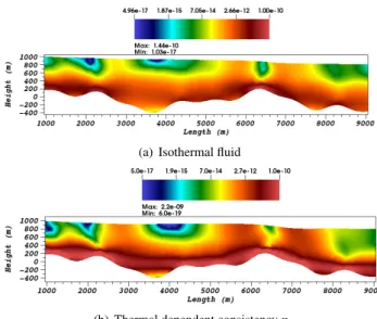
For both situations of sliding, the use of a temper-ature gradient to compute η0 (see (24)) leads to the
appearance of a distinct highly sheared layer close to the bottom (due to a higher temperature and thus a
(a) Isothermal fluid
(b) Thermal dependent consistency η0
Figure 9: Slip ratio r= 0.05: Computed shear-rate ˙γ for the observed
state (with n= 3) in s−1. The color scale is logarithmic.
(a) Isothermal fluid
(b) Thermal dependent consistency η0
Figure 10: Slip ratio r= 20: Computed shear-rate ˙γ for the observed
state (with n= 3) in s−1. The color scale is logarithmic.
smaller viscosity). At the surface, the areas of higher shear-rate inbetween those of very low shear-rate are larger and of higher absolute value. Conversely, the very low shear-rate spots close to the surface are more localized and of smaller absolute value.
Figure 11 plots the sensitivity to the consistency η0,
in the case of rapid sliding (r= 20), around a reference value ηm
0 = η0(Tm) which corresponds to a consistency
field evaluated for a constant temperature T taken
equal to the average temperature of the original thermal dependent flow Tm= −20◦C.
Similarly to the sensitivities with respect to the power-law exponent n, a correlation between the distribution of the gradient ∂ j/∂η0 and the shear-rate
map appears. However, the presence of the thermal physics make this correlation more vague; non trivial high sensitivity areas appear close to the surface when a thermal dependent consistency is used to generate the data. Conversely, the appearance of a high shear rate close to the bottom does not lead to a corresponding high sensitivity. The sensitivity maps, in the case of low sliding (r = 0.05), differ from Figure 11 but does not provide any additional insights on the influence of the thermal dependency in terms of surface velocities and is thus not plotted.
We point out that the differences in the steady
geometries of the surface with or without the thermal dependency are very small, even though a stiffening of the near surface fluid occurs.
6.3. Identification of η0 based on surface velocity
ob-servations
The following section is dedicated to the identifica-tion of a consistency field ηt
0(T ) computed using the
lin-ear thermal relation (24) with a temperature field
ob-tained with λ = 0.04 and plotted in Figure 12. The
computational domain and flows are identical to Sec-tion 5, i.e. the real Mertz glacier topography with either slow (r = 0.05) or rapid sliding (r = 20), but using a consistency η0computed from (24).
Cost function and initial guess. The cost function used for the identification is defined by:
j(η0; γ1, γ2)=
Z
Γs
kuobss − us(η0)k22 dx+ T (∇η0; γ1, γ2)
(25) where the synthetic data uobs
s are the horizontal
sur-face velocities perturbed by a 1% random Gaussian noise (the lack of robustness of these experiments lead us to consider a relatively small noise compared to the one used previously in the power-law index identifica-tion). The Tykhonov’s regularization term T (∇η0)
con-trols the oscillations of the control variable gradient. It is defined by: T (∇η0; γ1, γ2)= γ1 Z Γs k∂xη0k22dx+ γ2 Z Γs k∂zη0k22dx (26)
(a) Isothermal fluid (b) Thermal dependent consistency η0
Figure 11: Glacier flow with r= 20: sensitivity with respect to the consistency (∂ j/∂η0)(ηs0) around the state j(ηm0) (i.e. for an isothermal fluid at
−20◦
C) for an isothermal fluid (η0constant) and a thermal dependent one (η0defined by (24)).
Figure 12: Target consistency field ηt
0(in MPa.a
1/3) computed from
(24) and (12) with λ= 0.04 in
where the parameters γ1and γ2quantify the strength
of the imposed smoothness. The adjustment of these weights controls the degree of smoothness sought on the control variable. A classical approach, referred to as the Morozov’s discrepancy principle, consists of choosing γ1and γ2such that the final cost j(η
f 0; γ1, γ2)
matches the cost j(ηT
0; 0, 0) with the perturbed u obs
s (see
e.g.[37, 13]).
A layered consistency field decreasing from the surface to the bottom is sought. Therefore the balance on the gradients in both directions, appearing in the regularization term (26), is achieved using γ1 = γ2/7
(which corresponds to the exact ratio of the target consistency field). The exact ratio of 7 is not needed, but a very good guess (typically between 5 and 10) is required to achieve a decent identification.
Numerical results . The identification results are
plotted in Figure 14 and 15 for low and rapid sliding respectively. For each case, two inferred η0f are plotted corresponding to two different initial guesses which are ηi,m
0 = η0(Tm), Tm = −20◦C the average temperature
and ηi,g0 = η0(Tg), Tg= T(¯z, 0.02) with Ts= −30◦C (see
equation (23)). Evolutions of the cost function and the gradient along the minimization procedure for the two different initial guesses are plotted in Figure 13.
0 10 20 30 40 50
Iterations of the minimization procedure
102 103 104 105 106 107 108 109 1010 1011 1012 1013 1014 1015 1016
Absolute cost and gradient
Evolution of the cost for r=0.05 starting from ηi,m
0
Evolution of the gradient for r=0.05 starting from ηi,m
0
Evolution of the cost for r=0.05 starting from ηi,g
0
Evolution of the gradient for r=0.05 starting from ηi,g
0
Evolution of the cost for r=20 starting from ηi,m
0
Evolution of the gradient for r=20 starting from ηi,m
0
Evolution of the cost for r=20 starting from ηi,g
0
Evolution of the gradient for r=20 starting from ηi,g
0
Figure 13: Costs and gradients along the minimization cycle. They are plotted in absolute value in order to compare the results of the two
different initial guesses ηi,m
0 and η
i,g 0
From the evolution of the cost and the gradient, we can see that the behavior is more robust in the situation of moderate sliding (r = 0.05) for both intial guesses. In the case of rapid sliding (r = 20), the best intial guess ηi,m0 leads to a clearly better result (smaller cost and smaller gradient). The difference between the two intial guesses in the case of moderate sliding is not really significant. This observation is retrieved in the relative errors in Table 1. However, the most important information we have from Figure 13 is the fact that the decreasing of the gradient, regardless of the level of sliding or the initial guess, is much smaller (3 to 4 orders of magnitude) than for the identification of the rheological exponent n (20 orders of magnitude,
(a) Initial guess ηi,m0 (b) Initial guess ηi,g0
Figure 14: Slip ratio r= 0.05: Identified field η0fin MPa.a1/3. A lower bound of 0.1 on the consistency has been imposed to prevent the minization
procedure from generating negative values for η0.
(a) Initial guess ηi,m0 (b) Initial guess ηi,g0
Figure 15: Glacier flow with r= 20: Identified field η0f in MPa.a1/3. A lower bound of 0.1 on the consistency has been imposed to prevent the
minization procedure from generating negative values for η0.
see Figure 8) or the identification of the (β, n, m) triple (10 to 30 orders of magnitude, see Figure 17(a)). It brings to light the ill-posedness of the consistency identification problem.
The relative errors are given in Table 1. It clearly appears that the identification is easier in the case of low sliding. A small slip ratio represents a large contribution of viscous deformation to the surface velocities in favor of the identification of a rheological quantity whereas a higher slip ratio leads to a smaller contribution of the creep and of the rheology on the surface velocities.
It also makes sense in the light of the above sensi-tivities; the layered aspect of the sensitivity map in the case of low sliding (due to an important gradient of shear close to the bottom) helps to retrieve a layered
consistency field. In the case of rapid sliding the
distribution of the sensitivity is non trivial and so is the inferred consistency.
Discussion. Despite very good prior physical
knowl-edges introduced in the identification process (by using the exact ratio between horizontal and vertical
Slip ratio r= 0.05 r= 20
Initial guess Initial error Final error Initial error Final error
ηi,m0 63.90% 40.57% 63.90% 54.12%
ηi,g0 45.28% 35.49% 45.28% 41.31%
Table 1: Relative errorkη
f 0−ηt0k2
kηt
0k2 of the reconstructed rheological
con-stant for noise level δ= 1%.
consistency gradient, good initial guesses and a perfect knowledge of all the other physical parameters) and considering the noise level on the surface data of 1%, the resulting inferred consistency fields are poor. The basic layered aspect of ηt
0 is retrieved, thanks to
the anisotropic regularization, but the range is quite different from the target one and the presence of a rapid sliding significantly deteriorates the inferred consistency. As one can expect, the use of ηi,g0 as a first guess leads to a better identified consistency (see Table 1).
This result represents a major component of data as-similation that can be called equifinality of the system; an identical end state can be reached by different sets of parameters. In this situation, defining the end state as the horizontal surface velocities, ηt
0 and η
f 0 lead to
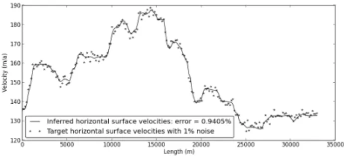
Figure 16: Normalized horizontal surface velocities: the plain line represents the computed surface velocities after identification and the stars represent the target surface velocities of the glacier flow consid-ered in section 6.3 perturbed by a 1% Gaussian noise. The error is the relative error between both sets.
ill-posed.
The present inverse results show that an uncertainty on the consistency do not greatly affect the bulk flow. Its inference is a strongly ill-posed problem. The target and inferred surface velocities are plotted in Figure 16 in the case of rapid sliding (r = 20) with ηi,m0 as a first-guess (which is the situation producing the larger relative error on the inferred consistency) to highlight the equifinality aspect.
Although physically questionable (in terms of di-mensions of the problem), identifications of a spatially varying power-law exponent n on the same situations lead to relative error of 0.076% and 1.86% on the low sliding and rapid sliding case respectively (with an initial guess n = 1), confirming the greater robustness of the identification of n.
These results suggest that the role of the thermal physics through the parameterization of the consistency is significantly minor compared to other parameters such as the basal friction or the power-law index. There-fore, the solving of a high precision model for the tem-perature field in the bulk could be pointless in the case of a power-law Stokes model and an assumed temperature profile should be sufficient. The present analysis cor-roborates a large scale numerical experiment performed in [38].
7. Identification of the scalar-valued triple (n, m; β) As observed here-before, a major quantity for the control of this type of flow is the friction coefficient β. The role of the slip ratio appears of great importance on the sensitivities and identification results on both the consistency and the rheological exponent by controlling
the flow regime.
The following numerical experiments are performed in the general context of an irregularly perturbed bottom (geophysical like topography), but again, both approaches are applicable for reproducible fluid flows observed during lab experiments.
In the case of ice flow for instance, it is well known that rapid sliding only occurs in the presence of a layer of subglacial sediment called till underneath the ice. Such a layer can for instance be modeled as a non-linear viscous fluid but a classical approach consists in using a non-linear viscous sliding law such as (11) to mimick this behavior.
7.1. Numerical experiments
The following numerical experiments aim to iden-tify at the same time the scalar rheological exponent n and the scalar sliding parameters β and m (see equation (11)). They are performed on the Mertz glacier flowline domain (see Figure 7) with a non-linear Poiseuille flow prescribed on the left boundaryΓland a lithostatic
pres-sure on the right boundaryΓr. A non-linear sliding law
with m = 3 (see equation (11)), and a uniform consis-tency η0are considered. In order to explore every
slid-ing situations, three average slip ratios are considered hereafter corresponding to r = 0.01, r = 1 and r = 40 (see equation (20)). The value r = 40 corresponds to the maximum slip ratio one can achieve for the present flow with complex topography. As further discussed, the local variation of the slip ratio can be large even for a given scalar friction coefficient β. Since scalar values are identified the cost function is simply:
j(n, m; β)= Z us(n, m; β) − u obs s (nt, mt; βt) 2 2 dx (27) The evolution of the cost j(n, m; β) (see (27)) and its gradient with respect to (n, m; β) along the data assimilation cycle is plotted in Figure 17. Figure 17(a) shows a robust identification for every situations; the decreasing of the costs is quite smooth (without taking into account the restarts of the minimization algorithm). The large drop of the gradient at the end highlight the fact that the optimum does not lie in a locally convex “valley” and it requires to run the minimization long enough to achieve the convergence even if the cost seems stable. We point out that such a result requires a sharp minimizer and accurate numerical schemes and
0 50 100 150 200 250 Iterations 10-36 10-33 10-30 10-27 10-24 10-21 10-18 10-15 1010-12 -9 10-6 1010-3 0
Relative cost and gradient Cost for rapid slidingGradient for rapid sliding Cost for intermediate sliding Gradient for intermediate sliding Cost for low sliding Gradient for low sliding
(a) Costs and gradients
0 50Iterations and sub-iterations of the minimization routine100 150 200 0.5 1.0 1.5 2.0 2.5 3.0 3.5
Rheological exponent n Identified parameter n with low sliding
Identified parameter n with intermediate sliding Identified parameter n with rapid sliding Target parameter n
(b) Rheological exponent n
0 50 100 150 200
Iterations and sub-iterations of the minimization routine 6 5 4 3 2 1 0 1 Fr ict ion co ef fic ien t lo g( β)
Target value log(β) for low sliding
Target value log(β) for intermediate sliding
Target value log(β) for rapid sliding
Identified parameter log(β) with low sliding
Identified parameter log(β) with intermediate sliding
Identified parameter log(β) with rapid sliding
(c) Friction coefficient log(β)
0 50 100 150 200
Iterations and sub-iterations of the minimization routine 1.0 1.5 2.0 2.5 3.0 3.5 4.0 4.5 5.0 Friction exponent m
Identified parameter m with low sliding Identified parameter m with intermediate sliding Identified parameter m with rapid sliding Target parameter m
(d) Friction exponent m Figure 17: Identification of the scalar-valued triple (n, m; β).
gradient. We also point out that this behavior is not sensitive to the first guess as long as the initial n is taken smaller than the target one.
7.2. Discussion
Inferred values. It clearly appears that the convergence of the rheological exponent n to the target value is achieved before the friction parameters β and m start their convergence. It demonstrates that n is a completely dominant parameter in the perspective of controlling the flow. Once n is almost converged, m followed by β start to converge to their target values. The errors on the inferred parameters for the different situations are given in Table 2. The final results are fully conclusive; all three parameters are well identified allowing to completely infer the flow regime from hori-zontal surface velocities only, under the assumption of uniform values for the three parameters. The plot of the resulting slip ratio in the case of low sliding (r= 0.01, see Figure 18) allows to understand the reason of a less faithful reconstruction of β and m. Indeed, a slip ratio
r = 0.01 corresponds to a situation where 1% of the
surface velocities come from the sliding and 99% come from the viscous deformation. Since a noise of 1% has been considered on the surface velocity data, it is a prioriimpossible to achieve an identification of the friction parameters. As we can see, the minimization
Slip ratio r= 0.01 r= 1 r= 40
n 0.111% 0.198% 0.332%
β 7.18% 0.225% 0.110%
m 15.8% 0.159% 0.332%
Table 2: Relative error for the reconstructed friction coefficient β, the friction exponent m and the rheological exponent n for different slip ratios.
procedure produced a pair (β, m) which provide the same surface velocities as the target one but leading to a higher slip ratio r = 0.016 to overcome the problem of the noise.
Topography/slip-ratio correlation. The surface veloc-ity data and the resulting surface velocities and basal velocities are plotted in Figure 18,19 and 20 for the three average slip ratios r = 0.01, r = 0.1 and r = 40 respectively.
The use of a scalar β as a friction coefficient can be seen as a simplified modeling approach. However, the non-uniform realistic topography considered here leads to a strongly non-uniform slip ratio with respect to the abscissa. In order to observe their variability of the basal state, the pointwise slip ratios and the opposite of the bedrock variations around its mean slope α (here α ∼ 2.10−2) are also plotted in Figures 18, 19 and 20 for the
Figure 18: Noisy data and inferred surface velocities, slip ratio and opposite of the bedrock variations for an average slip ratio r= 0.01
Figure 20: Noisy data and inferred surface velocities, slip ratio and opposite of the bedrock variations for an average slip ratio r= 40
three situations of sliding.
The case of rapid sliding (r = 40, the average
slip ratio), which allowed to obtain very accurate identification of the three quantities, shows a strongly
varying slip ratio; it oscillates between r = 7 and
r= 450 with large local gradients. A strong correlation between the variations of topography of the bedrock and the slip ratios peaks appears (see Figure 20). This aspect is a major component of the flow since it raises the question of the ability to separate the effect of the friction coefficient from the effect of the topography itself. As a matter of fact, in the ice flow context, the topography of the bedrock is generally the most poorly observed data (compared to the surface velocities and surface topography, see e.g. [39, 15]).
In the low sliding case (r = 0.01), although the
correlation between the slip ratio and the topography are not obvious, the slip ratio of the original flow and the one resulting from the identification are very similar in terms of variations.
In conclusion, the identification of the scalar-valued
triple (n, m, ; β) seems robust. In a more general
perspective of infering a spatially varying friction co-efficient β(x), such an identification allows to strongly constrain the flow and provide an excellent initial guess for a spatial identification of β. Nevertheless,
the observed correlation between the slip-ratio and the topography (mainly in the rapid sliding case r = 40) suggest a potential equifinality on the fric-tion/topography pair.
8. Equifinality problem of the friction/bed topogra-phy pair
In the geophysical context, the topography data are generally poorly (or not) observed and the potential correlation with the friction law is of prime interest.
The previous experiment raises a question about the dependency of the inferred friction coefficient on the topography and therefore the ability to separate the two effects. As a final experiment, a spatially varying friction coefficient is identified for a given reference topography and the corresponding reference surface velocity data (with a 1% Gaussian noise). These reference surface velocity data are then used to perform identifications of the friction coefficient β(x) for other topographies of the bedrock. The aim is to assess the link between the two quantities, depend-ing on the regime of sliddepend-ing, and the ability for the present inverse method to distinguish the two quantities.